MLPNN and Ensemble Learning Algorithm for Transmission Line Fault Classification
Abstract
Recently, Bangladesh experienced a system loss of 11.11%, leading to significant power cuts, largely due to faults in power transmission lines. This paper proposes the XGBoost machine learning method for classifying electric power transmission line faults. The study compares multiple machine learning approaches, including ensemble methods (decision tree, random forest, XGBoost, CatBoost, and LightGBM) and the multilayer perceptron neural network (MLPNN), under various conditions. The power transmission system is modeled using Simulink and the machine learning algorithms. In the IEEE 3-bus system, all of the learning types achieve approximately 99% accuracy in imbalanced and noisy data states, respectively, except CatBoost and decision tree, in the classification of line to line, line to line to line, line to line to ground, line to ground types of faults, and no fault. However, although all of the methods gain significant accuracy, assessing the performance results indicates that the XGBoost model is the most effective for transmission line fault classification among the methods tested, as it showed the best accuracy in the imbalanced and noisy state’s classification of faults, contributing to the development of more reliable and efficient fault detection methodologies for power transmission networks.
1. Introduction
A power system typically consists of three major parts: generation, transmission, and distribution. The electricity generated at the generation site is transmitted to the demand side via a power transmission system, which serves as a connector between them. Transmission lines play a crucial role in these systems by ensuring the proper delivery of generated power to the customer end. However, faults in power transmission lines are critical issues as they create instability, reduce reliability, and cause system discontinuities. Traditionally, fault detection relies on voltage and current measurements from the transmission line, which often require extended time to identify the fault, particularly in noisy and imbalanced data conditions—a common challenge in real-world scenarios.
For instance, in FY 2020-21, Bangladesh experienced a power transmission and distribution loss of 11.11% [1], and frequent power cuts severely affected businesses and discouraged foreign investment [2, 3]. Transmission line faults are one of the main contributors to these frequent power interruptions [4]. Therefore, detecting and classifying fault types rapidly is of utmost priority, as quick fault classification aids in swiftly locating and clearing faults, thereby increasing the reliability, stability, and continuity of the power system. Machine learning (ML), an advanced artificial intelligence technology, offers significant potential for fast and accurate fault classification within short periods [5].
Since the advent of ML, various approaches have been explored to classify transmission line faults. Prominent techniques such as support vector machines (SVMs), artificial neural networks (ANNs), and decision trees initially dominated due to their high performance [6–8]. SVMs are known for good data generalization and accuracy, while ANNs are noted for their quick learning capabilities, parallel data processing, and minimal tuning requirements [9]. Studies have employed backpropagation and autonomous neural networks to achieve notable speed and accuracy, although these models were not tested against noisy conditions [10–12]. Subsequently, advanced and hybrid techniques were proposed, such as DWT-based ANN, which performed under noisy conditions but suffered from accuracy degradation with varying signal-to-noise ratios [13]. Decision trees also demonstrated good accuracy but were often time-consuming.
Recently, ensemble learning techniques that combine multiple decision trees, such as random forest, Extreme Gradient Boosting (XGBoost), and CatBoost, have shown improved flexibility, accuracy, and performance [14–16]. A novel deep stack-based ensemble learning (DSEL) approach for fault detection and classification in photovoltaic arrays has demonstrated significant improvements in detection accuracy and robustness against noise and variability in input data [17]. Additionally, hybrid methods integrating discrete wavelet transforms with neural network algorithms, such as radial basis function networks, have proven effective in detecting high-impedance faults in distribution networks [18]. Similarly, AdaBoost ensemble models have been applied to photovoltaic arrays, highlighting the adaptability and effectiveness of ensemble learning approaches in diverse fault detection scenarios [19]. CatBoost, in particular, is noted for its effectiveness in handling imbalanced data [20].
Despite these advancements, existing models like SVMs, ANNs, and decision trees often fail to maintain high performance under varying conditions, such as different levels of fault resistance, distance, and load. This inconsistency underscores a critical research gap: the absence of a comprehensive evaluation of modern ML techniques designed to effectively handle these challenging conditions. This paper presents a detailed analysis of several ensemble learning algorithms, including decision trees, random forests, XGBoost, CatBoost, and Light Gradient Boosting Machine (LightGBM), in the context of transmission line fault detection and classification. By comparing the performance of these algorithms, this study aims to identify the most effective approach for enhancing fault detection accuracy and reliability in power systems.
Handling noisy and imbalanced data is a significant challenge in power system fault detection, as such conditions can degrade classification accuracy. Recent advancements have proposed various preprocessing and augmentation techniques to tackle these issues. Jalayer et al. [21] introduced a hybrid framework combining Wasserstein generative adversarial network (WGAN), convolutional LSTM (CLSTM), and weighted extreme learning machine (WELM) to enhance robustness against noise and imbalance. Similarly, studies utilizing SMOTEBoost [22] and variational mode decomposition demonstrated notable improvements in fault detection accuracy under adverse data conditions. Other recent works have highlighted filtering techniques and data augmentation strategies to improve noise robustness, ensuring models can reliably detect faults even in challenging environments [23]. Additionally, feature selection and balancing approaches, such as Synthetic Minority Oversampling Technique (SMOTE) and hybrid ensemble models, have been shown to handle class imbalances effectively [24]. These methodologies align closely with this study’s preprocessing techniques, including normalization and data augmentation, further validating the robustness of the proposed approach in addressing noisy and imbalanced datasets.
2. Objectives
- •
Evaluate and compare ML algorithms: Conduct a rigorous comparative analysis of various ML algorithms, including ensemble methods (decision tree, random forest, XGBoost, CatBoost, and LightGBM) and the multilayer perceptron neural network (MLPNN), to determine their performance in classifying power transmission line faults under diverse conditions.
- •
Assess accuracy and robustness: Measure the accuracy and robustness of these algorithms in handling noisy and imbalanced data, with specific attention to factors such as fault resistance, distance, and load, to evaluate their practical effectiveness.
- •
Identify the optimal fault detection model: Identify the most effective ML model by analyzing key performance metrics, such as classification accuracy, reliability, and operational resilience, to find the model that offers the best performance for real-world applications.
- •
Evaluate practical applicability: Test the applicability of the selected models using data from the IEEE 14-bus system, ensuring their effectiveness in managing diverse and challenging conditions typically encountered in power transmission systems.
This research introduces a novel comparative framework that evaluates both traditional and advanced ensemble learning techniques under challenging conditions, such as data imbalance and noise. Unlike prior studies, this work assesses not only the accuracy of these models but also their resilience to varying transmission line operating conditions. By focusing on a broad range of algorithms and conditions, this study offers new insights into the strengths and limitations of each approach, ultimately contributing to the development of more robust and accurate fault detection methodologies. By achieving these objectives, the study aims to significantly enhance the reliability and stability of power transmission networks, providing a foundation for future research and practical implementation.
3. Overview of Fault Detection
Fault detection in power transmission systems is crucial for grid stability and reliability. This involves analyzing electrical parameters like voltage and current and using mathematical models to classify faults effectively.
Fault detection relies on analyzing electrical signals to identify anomalies. Key components include the following.
3.1. Fault Current Calculation
3.2. Data Representation
Fault data are often noisy and imbalanced, requiring preprocessing techniques like normalization to improve ML model accuracy.
3.3. Mathematical Framework and Algorithmic Explanation
3.3.1. MLPNN
The mean squared error (MSE) is used as the loss function: .
MLPNNs can overfit, especially with small or noisy datasets. Their performance depends on hyperparameter choices and data quality.
3.3.2. Decision Tree
3.3.3. Random Forest
3.3.4. XGBoost
3.3.5. CatBoost
3.3.6. LightGBM
3.3.7. Handling Noisy and Imbalanced Data
Handling noisy and imbalanced data involves processing techniques like normalization, augmentation, and resampling. Techniques such as SMOTE are used to balance class distributions and enhance model performance.
4. Methodology
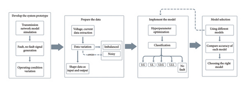
This section provides concise details of the simulation, data preparation, and model implementation.
Figure 1 illustrates graphically the overall idea of the working step by step.
4.1. Designing Power Transmission System
Figure 2 illustrates the power transmission system model, which is used to generate the training data for model implementation.
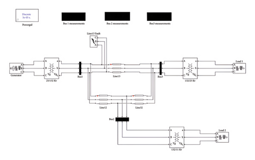
The transmission system has 3 buses, has a frequency of 50 Hz, and is operated at 132 kV with one generator and 2 loads connected at each end. The whole system is developed using the Simulink environment. Additionally, the zero and positive sequence parameters of the transmission line are considered. The sampling frequency of the generated three-phase instantaneous voltage and current signals is set to 1 kHz.
Table 1 the sampling frequency of generated three-phase instantaneous voltages and currents signal is 1 kHz. Besides, various operating conditions are also considered in the simulation. For example, signal is generated at fault resistance of 0.001, 50, and 100 Ω and fault distances of 50 and 100 km. Furthermore, a total of five types of faults—phase A to ground (AG), phase A to phase B (AB), phase A to phase B to ground (ABG), phase A to phase B to phase C (ABC), and no fault—are generated. These faults are simulated on transmission lines 12, 13, and 32. Sample waveforms for fault and no-fault conditions are shown in Figure.
| Parameters | Symbols | Value |
|---|---|---|
| Zero and positive sequence resistances (Ω/km) | R0, R1 | 0.0127, 0.0386 |
| Zero and positive sequence inductances (H/km) | L0, L1 | 0.9337, 4.1264 |
| Zero and positive sequence capacitances (nF/km) | C0, C1 | 12.74, 7.751 |
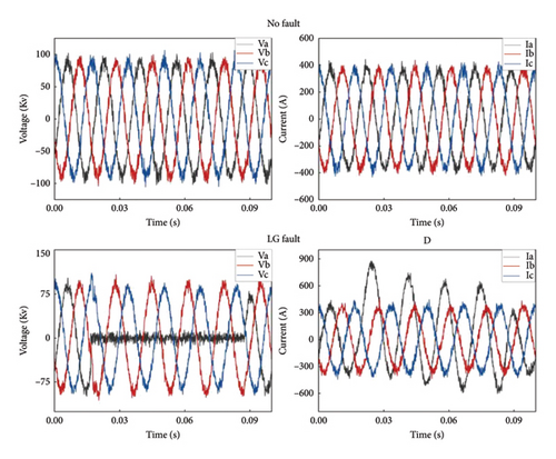
From Figure 3(a), it is clear that in the absence of fault, the voltage and the current waveform are sinusoidal, whereas when fault (Figures 3(b), 3(c), 3(d), and 3(e)) arises, it is seen that faulty phase voltages declined and the currents go up abruptly. Also, the waveform experienced heavy distortion.


4.2. Preparing the Data
After obtaining signals, it is required to achieve labeled datasets for model implementation. Thus, data are extracted from waveform using the Simulink model. For the classification task, the objective is to classify line to ground (LG), line to line (LL), line to line to ground (LLG), line to line to line (LLL), and no fault. Therefore, the dataset of 7440 data containing three-phase instantaneous voltages and currents labeled as the faulty and no-faulty state is prepared. Diversification of data (as discussed in Section 4.1) is made to ensure almost similar to real-world problems.
4.3. Implementing ML Models
The basic working principle of ensemble learning algorithms is shown in Figure 4.
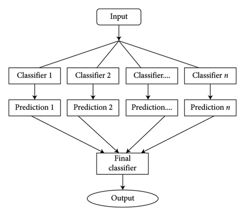
Figure 5 depicts the MLPNN model structure considered in this paper.
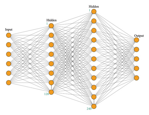
In MLP, the output of each node is the input of other successive layers. The input layer takes input values and passes the output to the additional connective (between input and output) layers referred to as hidden layers. At last, the output layer generates the result based on the input receives from the hidden layer.
However, MLPNN considered here contains input, output, and two hidden layers. In addition, the nonlinear activation function ReLU is used in hidden layers because for multilayers, it is obvious to use a nonlinear function. Otherwise, the network turns into a single-layer network that performs linear regression and cannot ensure linear separability. Since the problem output has probabilistic nature, softmax activation functions are used in the output layer, respectively, for categorical classification targets [34, 35].
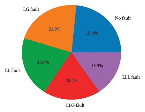
Finally, all of the models are implemented considering two categories of data. Figure 6 shows the imbalanced condition of the dataset used for classifying transmission line faults. It highlights the unequal distribution of data points across different fault types (e.g., LG, LL, LLG, and no fault). This imbalance poses a challenge for ML models, as it can lead to bias toward more frequent classes. The figure emphasizes the effectiveness of the studied models, such as ensemble learning methods and MLPNN, in handling this imbalance to achieve accurate fault classification.
Then, the model is examined for the second category, the noisy condition. To do so, additive white Gaussian noise is applied to the three-phase voltage and current signal. The added signal-to-noise ratio of Gaussian noise is 20 and 37 dB. Figure 7 shows some samples of the noisy waveform. Also, for achieving the best performance, the model hyperparameter is optimized as presented in Table 2.
| Model | Hyperparameter | Value |
|---|---|---|
| MLPNN | Activation function, optimizer, loss function | ReLU, sigmoid, “Adam,” “cross-entropy” |
| Decision tree | Number of trees, learning rate | 100, 0.1 |
| Random forest | 100, 0.1 | |
| XGBoost | 100, 0.1 | |
| CatBoost | 500, 0.5 | |
| LightGBM | 100, 0.1 | |
5. Results
5.1. Ensemble Learning–Based Algorithm
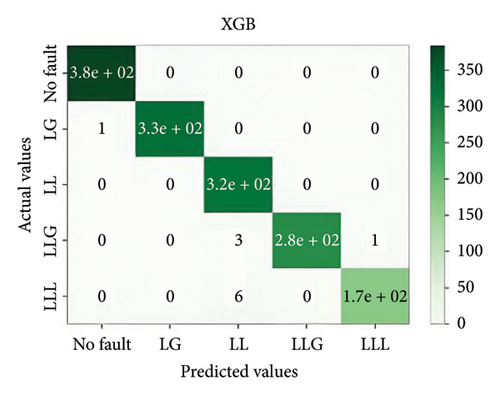
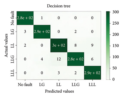
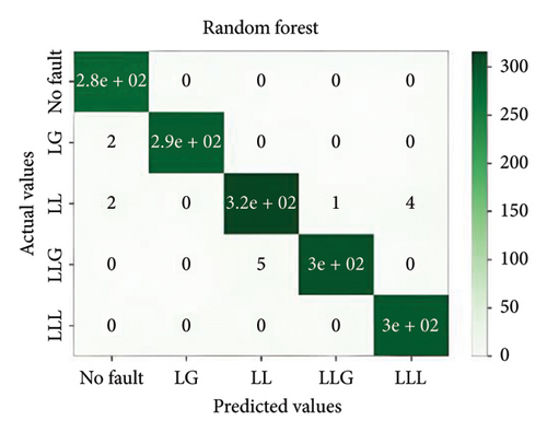
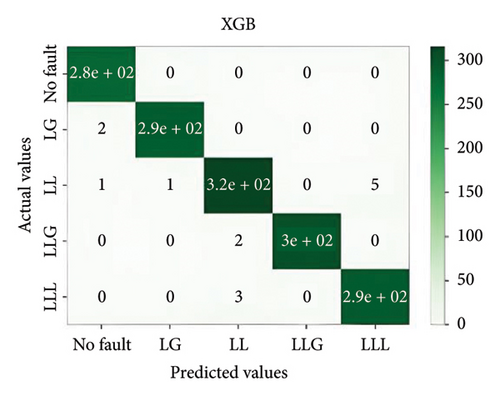
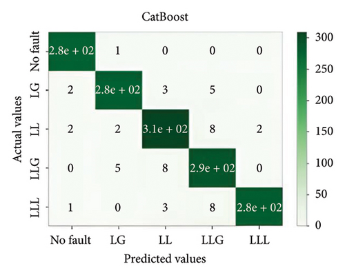
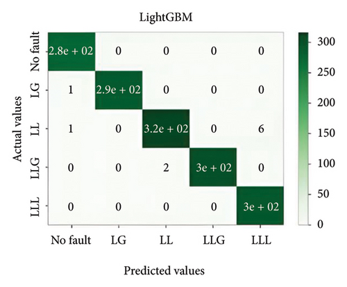
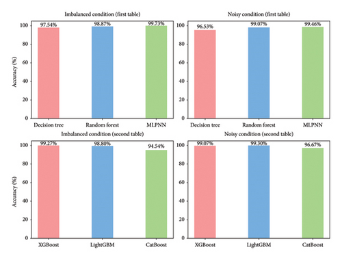
In general, ensemble learning is a learning technique that combines learning approaches iteratively to get a final prediction from an end model. It is quite popular because of its outstanding performance on class-imbalanced problems, noisy conditions, etc. [14]. In this work, two types of bagging ensemble methods such as decision tree and random forest and three types of boosting ensemble methods named as XGBoost, CatBoost, and LightGBM are implemented. In imbalanced data conditions, the models acquire 97.54%, 98.87%, 99.27%, 98.8%, and 94.54% accuracy, respectively, to classify the predefined types of fault. In noisy data conditions, the models also perform well. They acquire 96.53%, 99.07%, 99.07%, 99.3%, and 96.67% accuracy, respectively, to classify the faults. The confusion matrix is shown in Figure 8.




5.2. MLPNN
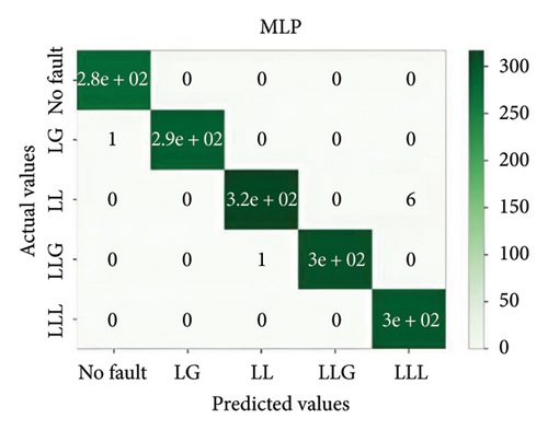
Similarly, MLPNN is also a good fit for the classification of faults in both conditions. Details of the results are described in Figure 9.

5.3. Performance on IEEE 14-Bus System
IEEE 14-bus system ideal model consists of 5 generators, 3 three-phase transformers, and 11 loads simulated by Bharath [36] taken for study to evaluate the developed methods. Fault 1 is generated in the transmission line between bus 1 and bus 2, and eventually, fault 2 and fault 3 are also created in the line between buses 6 and 13 and buses 2 and 4, respectively, as depicted in Figure 10. Two datasets—one noisy and one imbalanced—each consisting of 6000 data points, were generated for classification following the methodology outlined in Sections 4.1–4.3. These datasets assessed the model’s resilience under varying data conditions. Additionally, data collection was performed by varying fault resistance (0.1, 50, and 100 Ω), fault distance (50 and 100 km), and connected load (0.23 MW and 0.7 MW) to ensure diverse testing scenarios.
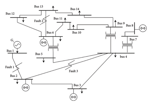
Figure 11 depicts the confusion matrix of the different models considered in this work when tested in IEEE 14-bus system.
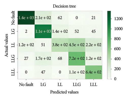

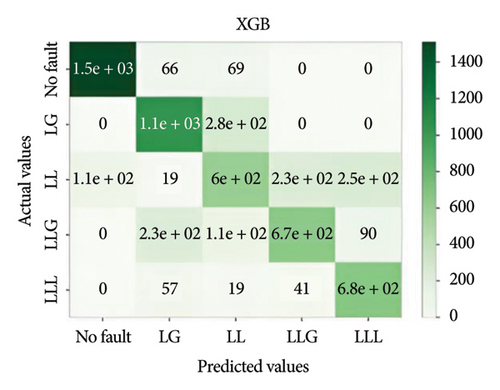
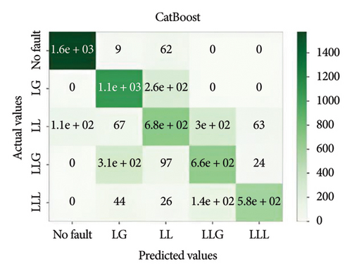
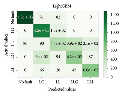
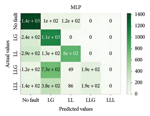
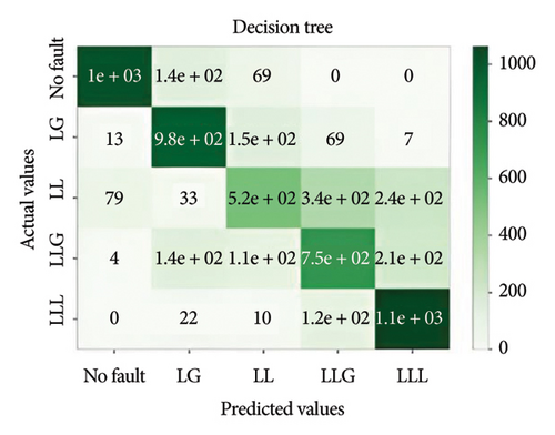
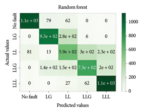
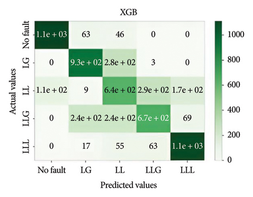
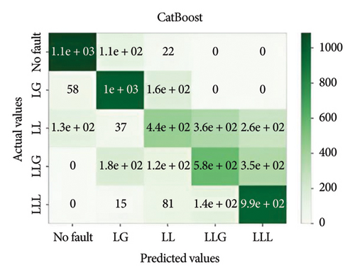

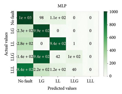
This study utilized the IEEE 14-bus system to validate the proposed models in a realistic and complex network. The results demonstrated that XGBoost maintained high accuracy and robustness under diverse fault conditions, highlighting its practical applicability for standard power systems.
It is important to evaluate the method’s performance briefly. Tables 3, 4, 5, and 6 discuss the precision, recall, F1, and accuracy score of the methods for classification tasks. The results indicate that all methods perform well in the 3-bus system. However, in the test case, while ensemble learning algorithms maintain high accuracy under both balanced and noisy conditions, MLPNN exhibits a notable decline in accuracy in both scenarios. Among all the models, XGBoost demonstrates the best performance, achieving approximately 74% accuracy. However, it also depicted that the best performative model among all the models is XGBoost by gaining almost 74% accuracy.
| Data type | Model name | Precision | Recall | F1 score | Accuracy (%) |
|---|---|---|---|---|---|
| Imbalanced | Decision tree | 0.97 | 0.97 | 0.97 | 97.54 |
| Random forest | 0.99 | 0.99 | 0.99 | 98.87 | |
| MLPNN | 1 | 1 | 1 | 99.73 | |
| Noisy | Decision tree | 0.97 | 0.97 | 0.97 | 96.53 |
| Random forest | 0.99 | 0.99 | 0.99 | 99.07 | |
| MLPNN | 1 | 1 | 1 | 99.46 | |
| Data type | Model name | Precision | Recall | F1 score | Accuracy (%) |
|---|---|---|---|---|---|
| Imbalanced | XGBoost | 0.99 | 0.99 | 0.99 | 99.27 |
| LightGBM | 0.99 | 0.99 | 0.99 | 98.80 | |
| CatBoost | 0.95 | 0.95 | 0.95 | 94.54 | |
| Noisy | XGBoost | 0.99 | 0.99 | 0.99 | 99.07 |
| LightGBM | 0.99 | 0.99 | 0.99 | 99.30 | |
| CatBoost | 0.97 | 0.97 | 0.97 | 96.67 | |
| Data type | Model name | Precision | Recall | F1 score | Accuracy (%) |
|---|---|---|---|---|---|
| Imbalanced | Decision tree | 0.69 | 0.69 | 0.68 | 68.84 |
| Random forest | 0.74 | 0.74 | 0.74 | 74.1 | |
| MLPNN | 0.57 | 0.57 | 0.56 | 57.59 | |
| Noisy | Decision tree | 0.71 | 0.71 | 0.70 | 70.92 |
| Random forest | 0.73 | 0.73 | 0.73 | 73.07 | |
| MLPNN | 0.49 | 0.48 | 0.49 | 49.73 | |
| Data type | Model name | Precision | Recall | F1 score | Accuracy (%) |
|---|---|---|---|---|---|
| Imbalanced | XGBoost | 0.74 | 0.74 | 0.74 | 74.18 |
| LightGBM | 0.72 | 0.72 | 0.71 | 72.34 | |
| CatBoost | 0.75 | 0.75 | 0.75 | 75.16 | |
| Noisy | XGBoost | 0.73 | 0.73 | 0.73 | 73.00 |
| LightGBM | 0.73 | 0.73 | 0.60 | 70.00 | |
| CatBoost | 0.66 | 0.67 | 0.66 | 66.93 | |
The following charts in Figure 12 represent the accuracy percentages of various classification models under imbalanced and noisy conditions for IEEE 3-BUS.
The following charts in Figure 13 represent the accuracy percentages of various classification models under imbalanced and noisy conditions for IEEE 14-BUS.
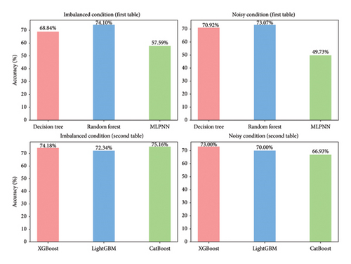
Not only is accuracy a general measure of the effectiveness of a model but also it does not address class imbalance–related challenges faced by the model. For this reason, the values of precision, recall, and F1 score are calculated for each of the models. These yield indicative metrics regarding how the model identifies true positives (recall), avoids false positives (precision), and balances the two (F1 score). For example, XGBoost generated an F1 score of 0.99 with respect to imbalanced conditions and 0.73 for the IEEE 14-bus test, signifying the robustness with the compromise in noise. Most of the models impart consistent recall that makes them trustworthy in detecting faults, while precision ensures less false alarms. This complete evaluation gives every indication that ensemble techniques work well in data with imbalanced distributions.
6. Discussion
6.1. Computational Efficiency and Scalability
For practical applications, the implemented models’ scalability and computing efficiency are essential. As a gradient boosting technique, XGBoost excels in processing speed because of its parallel tree-building methodology, which drastically cuts down on training time. Nevertheless, the computational cost of the dataset may rise with increasing feature dimensions and size, requiring careful adjustment of hyperparameters like learning rate and tree count. Large-scale power systems can benefit from XGBoost’s scalability, although real-time applications may encounter difficulties due to hardware constraints. In contrast, less complex models such as decision trees require less computing power, but they may lose accuracy in noisy environments. To guarantee scalability for big data scenarios, future research should investigate methods like distributed computing and model optimization.
6.2. Practical Insights on XGBoost
XGBoost is recommended as the most effective model due to its superior accuracy, robustness to noise, and ability to handle imbalanced data. However, its practical adoption in real-world systems requires consideration of operational speed and cost. XGBoost’s fast training process, achieved through advanced optimization techniques, supports its deployment in systems requiring frequent updates. Nonetheless, its reliance on multiple hyperparameters demands computational resources, which may increase costs, particularly for resource-constrained systems. Additionally, XGBoost’s performance may degrade under extremely noisy conditions or with insufficient data preprocessing. For transmission systems with varying fault resistances and load conditions, hybrid methods integrating XGBoost with signal denoising techniques can further enhance reliability.
6.3. Limitations
While this study provides valuable insights into fault classification using ML methods, certain limitations must be acknowledged.
6.3.1. Reliance on Simulink-Generated Data
The dataset used for model training and testing is generated in a controlled simulation environment using MATLAB Simulink. Although the dataset incorporates noise and imbalance to emulate real-world conditions, it may not fully represent the complexities of real-world transmission systems. Future work should validate the proposed models on actual transmission line data to enhance their applicability.
6.3.2. Simplified Test System
The study primarily uses a 3-bus system and partially validates the models on the IEEE 14-bus system. While these systems are effective for initial testing, larger and more complex networks, such as the IEEE 118-bus or 300-bus systems, would better demonstrate the scalability and robustness of the methods. This will also enable direct benchmarking with existing research using standard test systems.
6.3.3. Scalability Challenges
Although the study demonstrates high accuracy under imbalanced and noisy conditions, the computational cost associated with XGBoost and other ensemble methods may pose scalability challenges for large-scale systems. Developing lightweight implementations and optimizing hyperparameters for real-time deployment should be explored in future work.
The research work initially employed a simplified 3-bus system for preliminary testing. To ensure broader applicability and robustness, we extended the evaluation to the IEEE 14-bus system, a standard network widely used in power system studies. The IEEE 14-bus test case included variations in fault resistance, distance, and load, enabling a rigorous assessment of model performance under realistic operating conditions.
While the 14-bus system provides significant insights, future work could extend the analysis to larger standard networks, such as the IEEE 118-bus or 300-bus systems. This would allow for further evaluation of model scalability and performance in complex grid scenarios.
7. Conclusions
Overall, after the comparative evaluation of performance metrics, this paper presents that it is crystal clear that the better performative learning algorithms are boosting ensemble learning types (XGBoost, CatBoost, and LightGBM), and among them, the best performative model is XGBoost which attained 99.27% and 99.07% accuracy, respectively, toward imbalanced and noisy state fault classification of power transmission line. In addition, the proposed XGBoost model has also resilience toward transmission line operating condition (fault resistance, distance, and load) variations. While this study relies on Simulink-generated data, the dataset was designed to closely emulate real-world conditions by incorporating varying fault resistances, distances, and noise levels (Gaussian noise at 20 and 37 dB). These conditions simulate practical transmission line scenarios, making the findings relevant and meaningful.
Testing with real-world transmission data is indeed crucial for validating the robustness of the proposed models. However, acquiring such data often requires collaboration with utility companies and access to sensitive infrastructure, which is currently beyond the scope of this work. As a next step, we aim to explore partnerships or open-access datasets to further validate the findings in future research.
Finally, as the area of ML is continuously evolving, there should be a scope to explore XGBoost with other deep learning models and develop an intelligent, automotive protective system for power transmission system by isolating the faulty section.
Conflicts of Interest
The authors declare no conflicts of interest.
Funding
This research was conducted without any internal and external funding. The authors only utilized institutional resources and support provided by the Department of Electrical & Electronics Engineering at Sylhet Engineering College and Shahjalal University of Science & Technology, Sylhet, Bangladesh.
Open Research
Data Availability Statement
The datasets used and analyzed during this study were generated from MATLAB Simulink for the simulation of power transmission line faults. These datasets are available from the corresponding author upon reasonable request.


