2.1. Well Information

The target field, located in Central Asia, has been producing hydrocarbon for several decades. During the Paleozoic era, it was the site of extensive deposition of deep marine sediments and platform carbonates within a passive margin setting. The commencement of the Ural orogeny toward the late Paleozoic era marked a significant shift in tectonic dynamics, transitioning the depositional environment from a deep marine setting to a more varied shallow marine and fluvial landscape during the Jurassic period. This tectonic evolution facilitated the accumulation of sand deposits with thicknesses varying between 5 and 20 m, interspersed with layers of claystone and coal within the Jurassic stratigraphic interval. These juxtaposed subformations are instrumental in forming the primary reservoir-seal rock assemblages within the exploration field. The Jurassic sand reservoirs are notably situated at true vertical depths ranging between 2400 and 3100 m. The replenishment of these sand units is predominantly influenced by the dynamics of meandering to braided channel systems, which serve as the chief conduits for sediment transport and deposition. The variability in channel directionality over temporal scales has significantly contributed to the geological complexity, with sand deposition predominantly concentrated along the routes of ancient channel pathways, thus enhancing the reservoir’s heterogeneity.

Approximately 10 vertical wells have been drilled annually in the target field, with the average drilling time of about 25 days. Prior to the initiation of drilling operations, the conductor is installed through hammering. A typical well design is divided into three sections: Section I is up to a depth of 100 m with a 13 3/8 in. surface casing (and a hole inner diameter of 17 1/2 in.); Section II is from 100 to 800 m depth with a 9 5/8 in. casing; and Section III is from 800 to 3100 m depth with a 7-inch casing. Bit replacement was circumvented within a designated each section barring unusual circumstances, which is for minimizing nonproductive time.

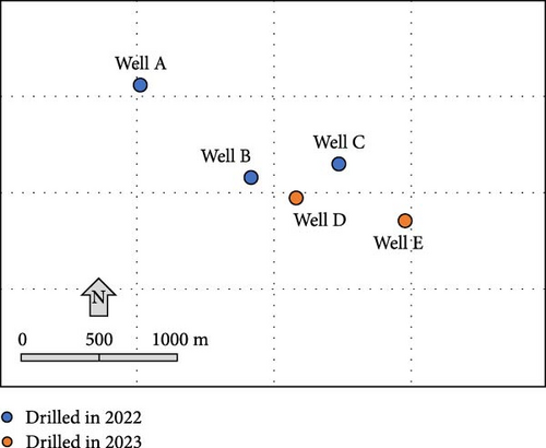
ROP prediction in this study concerns on Section III and five wells, three wells drilled in 2022 (namely, Well A, Well B, and Well C) and the remaining two (namely, Well D and Well E) drilled in 2023 (Figure 1).

2.2. Preparation of Input Dataset

2.2.1. Well-Logs and Drilling-Operation Data

Six types of well-log data were available for all wells: density (RHOZ), sonic (DT), gamma ray (GR), resistivity (RT), neutron porosity (TNPH), and photoelectric factor (PEFZ) (Table 1). The measured depth (MD) ranges for the well-logs spanned from 817 to 3030 m with a data interval of 0.2 m, identical to ROP recorded. Each well provided 11,066 instances of well-log data. The drilling-operation data encompass WOB and RPM. The several thousand measurement points of mud-logging and wireline logging in each well are depth-matched by GR measurements so that any possibilities of mismatches in data points are not needed to be considered.

Table 1. Well-logs and drilling operation parameters as the input dataset in the study.

Data type	Abbreviation	Unit
Well-logs
Bulk density	RHOZ	g/cm3
Sonic travel time	DT	μs/m
Gamma ray	GR	gAPI
Formation resistivity	RT	Ω·m
Neutron porosity	TNPH	Fraction
Formation photoelectric factor	PEFZ	Barns/electron
Drilling-operation Parameters
Weight on bit  Rotary speed	WOB RPM	Ton r/min

Figure 2 illustrates the data series acquired from Well A. Except for ROP as the output response, the other parameters were normalized and thereafter utilized as the input dataset. Herein, no preprocessing for the other is employed, which means data that may seem to be outliers are also regarded as characteristics of formations.

2.2.2. Denoising ROPs (Output) With Kalman Filter

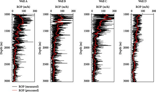
The ROP data series, as illustrated in Figure 2, exhibits complex fluctuations, emphasizing the need to extract the overall trend rather than concentrating on individual data points in establishing a meaningful correlation between the ROPs and the input data. In this study, Kalman filter is used as a method of denoising. It can provide data trends denoised by filtering out random fluctuations which can be regarded as measuring errors as explained below.

Kalman filter estimates the state of a system and subsequently compares this estimated with observed values [27, 28]. This approach acknowledges the inherent uncertainty in both the estimated and observed values. By addressing the discrepancies between two values, the algorithm successively refines its estimation for future data by considering the relevant uncertainties. Through iterative state update processes based on the new observations, Kalman filter can estimate the state by reducing the estimation error effectively according to time increase (depth deepening in this study). The process is summarized as Equation (1) for estimation and Equation (2) for state update:

$$ (1)

$$ (2)

In Equation (1), x, P, and Q denote the estimated state, the state variance matrix, and the process variance matrix, respectively, where the subscript t|t signifies the current time step, the subscript t − 1|t − 1 indicates the prior time step, and the subscript t|t − 1 is the intermediate time step. In Equation (2), R represents the measurement covariance, K the Kalman gain, and y the observation variable. The sequential updates Equations (1) and (2) by trial-and-error to get the improved relation between log and ROP data.

The results of denoising the ROPs for each well are shown in Table 2 and Figure 3. Relative to the original data, the denoised ROPs demonstrate a reduction in the coefficient of variation, with the mean essentially unchanged, and a narrower span between the maximal and minimal values noted. The red lines in Figure 3, depicting the denoised ROPs, validate the observed ROP trend patterns. It shows the extent of the fluctuation is similar to that of WOB data which have larger influences on the ROP compared to the RPM data among the drilling parameters (Figure 2). The ratio of 1:200 for process covariance and noise covariance, based on the trial-and-error method, was applied to get the reliable R² values.

Table 2. Statistical results of denoising ROPs using Kalman filter.

Dataset	Coefficient of variation	Mean	Maximum	Minimum
Well A
Raw	0.451	41.045	251.207	0.628
Denoised	0.064	41.257	113.924	4.106
Well B
Raw	0.397	45.343	275.052	0.394
Denoised	0.053	45.279	127.309	10.021
Well C
Raw	0.427	50.759	584.887	0.798
Denoised	0.053	50.790	196.432	10.084
Well D
Raw	0.308	38.413	130.664	1.398
Denoised	0.052	38.350	96.709	7.115

• Note: The coefficient of variation is defined as the ratio of the standard deviation to the mean.
• Abbreviation: ROPs, rate of penetrations.

2.2.3. Litho-Facies Classification Using K-Means Clustering

Despite the fact that depositional features and in situ rock properties have been shown to influence the ROPs [29], available litho-facies, a geological information for rock groupings based on the similar sedimentary conditions, at specific depths often remains elusive. Consequently, in constructing a workflow that addresses rock distribution heterogeneity with depth, particularly in scenarios with scarce core data, we aim to incorporate rock characteristics distinguishable via unsupervised learning-based clustering utilizing well-log data.

This work uses K-means clustering, one of unsupervised methods for classifying the big-data, to categorize well-log data features. Metrics, including the silhouette score (s(i)), and the Davies–Bouldin index (DBI), are employed to derive the optimal number of clusters (refer to Equations 3 and 4) [30]. The s(i) encapsulates how similar an individual data point is to its cluster compared to other clusters, by evaluating the extent of similarity in intracluster against intercluster separation. Meanwhile, the DBI gauges the quality of clustering by calculating the mean similarity between each cluster and its nearest counterpart. This measure depends on the ratio of intracluster to intercluster distances, where a higher s(i) and a lower DBI signify superior clustering by minimizing distances within clusters and maximizing those between them:

$$ (3)

$$ (4)

In Equation (3), a(i) denotes the mean distance between a sample, i, and all other points in the same cluster, whereas b(i) represents the mean distance from a sample, i, to all points in the nearest other cluster. Equation (4) defines k as the total number of clusters, σ_i as the mean intracluster distance for cluster i, and d(c_i, c_j) as the centroid distance between clusters i and j. Table 3 compares the calculated values of s(i) and DBI for several numbers of clusters. From this, the optimal number of the clusters is derived as three, evidenced by the highest s(i) and the lowest DBI. These clusters have been designated as C0, C1, and C2, respectively.

Table 3. Comparison of s(i) and DBI values for deriving the optimal number of clusters.

Number of cluster	Silhouette score	Davies–Bouldin index
2	0.4107	0.9476
3	0.4180	0.9232
4	0.3389	1.0468
5	0.3036	1.1646
6	0.2994	1.0985
7	0.2950	1.0636
8	0.2931	1.1419
9	0.2918	1.0876

• Note: The bold means that we select 3 as the optimum number of cluster.

Figure 4 shows the clustering results based on the principal component analysis (PCA). It validates the clustering methods by showing distinct data segmentation. Figure 5 offers box-whisker plots that explain the statistical dispersion of well-log data within each cluster. Through PCA results and box-whisker plots, extraction of three clusters from well-logs seems to be adequate qualitatively.

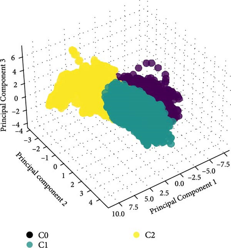
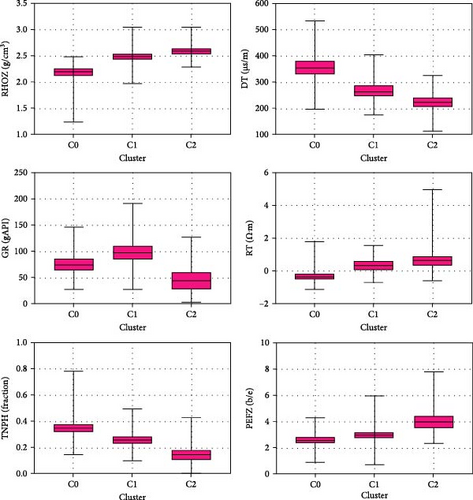
As a result of clustering, cluster C0, which has the highest DT and the lowest RHOZ relative to other clusters, is inferred to exhibit porous and soft attributes, indicating undercompaction within the shallow interval and its portion decreases gradually as depth is getting deeper due to the increase of the compaction. Cluster C1, which has intermediate characteristics between C0 and C2 by higher RHOZ and RT than C0, is inferred to be moderately harder and tighter than C0. C2, with the highest RHOZ, the lowest DT, and the lowest GR among the three clusters, signifies the hardest formations.

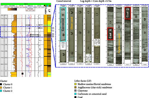
Figure 6 also validates the clustering results by showing the comparison to available core data analysis which is highlighted within a blue dotted box. Within the coring interval, the majority of the data belongs to the C1 cluster, which indicates the facies of sandstone; meanwhile, some data points indicate clusters C0 and C2 with coal and carbonate or cemented sand, respectively. From the well-log and core data, the exact alignment of the depths for C0 and C2 validates the effectiveness of data-driven clustering. Based on the core data analysis, Table 4 summarizes litho-facies corresponding to each cluster.

Table 4. Well-log/core characteristics of three clusters and the inferred litho-facies.

Cluster	Well-log/core characteristics	Inferred litho-facies
Cluster 0 (C0)	Low GR and high porosity-related log values (RHOZ, DT, and TNPH) imply a porous and clay-lean characteristic Corresponded to interbedded coal layers (depth > 1500 m) or shallow sand intervals (<1500 m)	Undercompacted sand, claystone, intercalated coal (soft characteristic) High ROP supports the soft characteristic
Cluster 1 (C1)	Moderate log characteristic between clusters 0 and 2 A wide range of GR values implies a relatively high variation in clay volume Corresponding to argillaceous to clean sand intervals in the Jurassic cored section	Compacted, argillaceous to clean sand (moderate characteristic)
Cluster 2 (C2)	Highest RHOZ, highest RT, lowest GR, and lowest DT imply a dense, resistive, and hard characteristic with clay-lean composition PEF near 5 suggests limestone rather than sand Corresponded to the Cretaceous carbonate interval or calcite cementations in the Jurassic sand interval	Carbonate or calcite–cemented sand (hard characteristic) Low ROP supports the hard characteristic

• Abbreviations: GR, gamma ray; ROP, rate of penetration.

3.1. Data Interrelationship and Deep-Learning Architecture

It is important to examine the asymmetric interrelationships among the data to test whether a deep-learning predictive model is applicable. If a particular input value has a very high correlation linearly with the response, the result can be estimated only with this input without the need to build the deep-learning model.

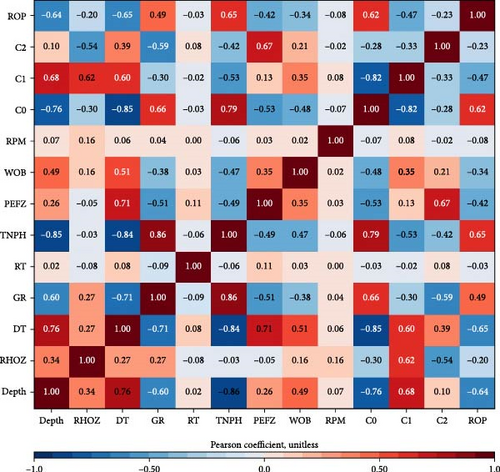
The Pearson correlation coefficient measures a linear correlation between two variables. Figure 7 depicts a heat map of the Pearson correlation coefficient. The MD, DT, TNPH, and C0 reveal the Pearson correlation coefficient of absolute value greater than 0.6 with ROP, indicating a higher linear correlation compared to other data. Figure 7 confirms that no specific data solely determines the ROP and thereby it requires elucidating the nonlinear relationships by developing the deep-learning architecture.

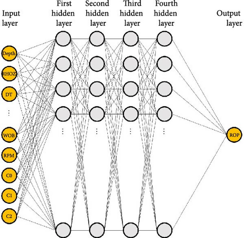
The deep-learning architecture developed in this work is based on deep-neural-network with fully connected layers for a regression purpose. Table 5 summarizes the input and output dataset. Ten kinds of input data are used, categorized by the MD, the well-logs, the drilling operation, and litho-facies, while one output value is the ROP. Except for the litho-facies s, all input data are normalized. The litho-facies information clustered by the well-logs is a vector-typed one-hot encode, i.e., C0 = (1, 0, 0), C1 = (0, 1, 0), and C2 = (0, 0, 1). The deep-learning architecture has four hidden layers which have 50 neurons each. It employs the learning rate ( = 0.0001), the mini-batch size ( = 64) based on hyperband method and its fine-tuning technique (Figure 8). The activation function, the optimizer, and the loss function are ReLU, ADAM, and the mean absolute error (MAE), respectively.

3.2. ROP Predictive Models: Effects of Litho-Facies and Transfer Learning

The production performances which have been drilled before are not similar to each other in the target field. It seems to be due to that the horizontal heterogeneity is severe by the complex depositional environments. This severe heterogeneity hinders the ROP prediction based on only well-logs of the offset wells and thus it requires to examine the effects of input dataset as well as of any tuning methods. Notably, unlike this traditional deep-neural-network, this study examines the ROP predictability by incorporating the transfer learning because the number of available wells is limited, which makes it difficult to reproduce or expand the training dataset. The transfer learning utilizes a pre-existing learning patterns as a starting point for a similar or related task [31].

To test the ROP prediction performances based on different input datasets, this work is divided into three cases: W4 uses only well-logs and drilling operation data as input values for the deep-learning model, excluding the log-based litho-facies. W4 represents four wells, namely Well A to D. The second scenario, referred to as W4C, includes the litho-facies information in addition to the input data used in W3. The last case is W4C-T, involved combining transfer learning with W4C (Figure 9; Table 6). W4C-T assumes that the data series of Well E is similar to those of Well D so that the tuning of weights at the last hidden layer is carried out using Well D. The training and validation groups were randomly divided in an 8:2 ratio. The test data are those of Well E.

3.3. Indicators to Evaluate the Prediction Performances

In Equations (5)–(7), y_i denotes the actual ROP at the ith depth, while $$ represents the ROP estimated by the predictive model at the ith depth. $$ is the arithmetic mean of the ROPs. $$ indicates the distance between y_n and $$, and $$ signifies the cumulative distance between y_n−1 and $$. R² is a statistical indicator that determines the proportion of variance in the measured ROPs (the true values) that can be explained by the predicted ones. MAE is a measure of error while DTW measures the similarity between two time series, that is, the measured and the predicted ROPs.

4.1. Evaluation of ROP Prediction Accuracy

Figure 10 depicts the ROP prediction results of deep-learning models such as W4, W4C, and W4C-T. At shallow depths, ROP shows significant variation, but as depth increases and the formation consolidation intensifies, ROP decreases. Since the ROP prediction model is trained using denoised well-logs, there are limitations in accurately predicting the sharply changing ROP with depth. However, it effectively tracks the overall trend of ROP variations. R², indicative of the regression model’s characteristics, improves from 0.49 for the basic model (W4) to 0.57 when litho-facies information through K-means clustering is included (W4C) and further to 0.73 when both transfer learning and litho-facies information are incorporated (W4C-T). This improvement is attributed to the expanded dataset used for training, enhancing the accuracy of ROP predictions. As the heatmap in Figure 7, all data are nonlinearly linked to the ROP, validating the applicability of predictions through the deep-learning model. The right-hand side of Figure 10 illustrates that while the error between actual and predicted ROP values is minimal at lower ROP values, it increases as the ROP values grow. This result indicates the requirement for improved prediction performance at shallow depths, where ROP variability is high. A reason for the low prediction performance in high-variability sections can be traced to noise removal from input well-logs using Kalman filter.

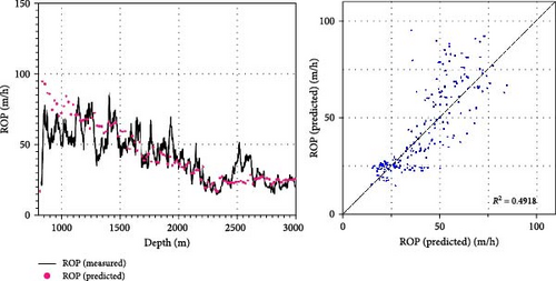
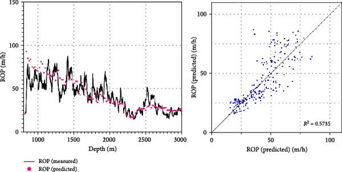
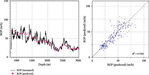
Figure 11 plots MAEs for each 100-m segment of the entire drilling section (from 800 to 3100 m). While W4 and W4C exhibit high MAE values in shallow depths where ROP variability is high, W4C-T demonstrates overall lower and more consistent trends. MAE of W4 model is 8.82 m/h, whereas it decreases to 6.79 m/h in the W4C-T model. This result proves that the deep-learning predictive model incorporating litho-facies information and transfer learning not only has lower errors but also offers better prediction performances in sections with high ROP variability. Table 7 summarizes the performance evaluation metrics. DTW of W4 is 473, while W4C-T has 361. This improvement indicates enhanced similarity between the actual measured ROP trends and the predicted values.

In summary, compared to the base model, W4C-T model demonstrates significant improvements in prediction performance, with an increase in R² by 49% ($$), a reduction in MAE by 23% ($$), and a decrease in DTW by 24% ($$). The improvement of prediction accuracy emphasizes the limitation of basic model and the necessity of transfer learning for coping with local heterogeneity or inconsistency of newly acquired data.

4.2. Optimization of WOBs to Reduce Drilling Time

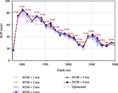
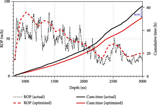
Using the most reliable ROP predictive model, that is, W4C-T, the paper examines the possibility to reduce drilling time by optimizing ROPs. The ROP prediction in this study, analyzed postdrilling, can provide guidelines for subsequent drilling operations. Generally, when RPM is fixed for safety reasons, WOB can be used as a drilling operation factor. Since varying WOB over short intervals can pose practical challenges in drilling operations, this paper segments the entire drilling interval into 100-m sections. For each section, WOB values ranging from 1 to 6 tons are assigned, and a WOB scheduling is optimized to obtain the maximum ROPs. Figure 12a illustrates the predicted ROP for each 100-m segment according to different WOB values, with the optimized values indicated by a dashed line connecting the WOB values yielding the highest ROP. By scheduling WOB for each segment, the total drilling time could be reduced by ~16.5% compared to the actual drilling time of Well E (Figure 12b). In addition, these WOB guidelines for each segment allow for efficient preparation for the next drilling operation.

This study developed a reliable deep-learning model capable of predicting ROP by extracting litho-facies information from well-log data and performing transfer learning from offset wells, particularly in regions with limited core data and high heterogeneity. By fixing RPM and optimizing WOB by segment, WOB scheduling to reduce drilling time is proposed. The results of this study demonstrate that in highly heterogeneous regions, reliable ROP prediction techniques can be achieved through preprocessing and integrated analysis of well-log data.