International Journal of Energy Research

Volume 2024, Issue 1 5544635

Research Article

Open Access

A Data-Driven-Aided Thermoelectric Equivalent Circuit Model for Accurate Temperature Prediction of Lithium-Ion Batteries

Junting Bao,

Junting Bao

orcid.org/0009-0003-2006-5717

College of Information Engineering , Zhejiang University of Technology , Hangzhou , China , zjut.edu.cn

Search for more papers by this author

Yuan Mao,

Corresponding Author

Yuan Mao

[email protected]

orcid.org/0000-0002-7921-0507

College of Information Engineering , Zhejiang University of Technology , Hangzhou , China , zjut.edu.cn

Search for more papers by this author

Zhiming Zhang,

Zhiming Zhang

REPT BATTERO Energy Co. Ltd , Wenzhou , China

Search for more papers by this author

Yajie Jiang,

Yajie Jiang

School of Electrical and Electronic Engineering , Nanyang Technological University , Singapore , Singapore , ntu.edu.sg

Search for more papers by this author

Youbing Zhang,

Youbing Zhang

College of Information Engineering , Zhejiang University of Technology , Hangzhou , China , zjut.edu.cn

Search for more papers by this author

Yun Yang,

Yun Yang

School of Electrical and Electronic Engineering , Nanyang Technological University , Singapore , Singapore , ntu.edu.sg

Search for more papers by this author

Junting Bao,

Junting Bao

orcid.org/0009-0003-2006-5717

College of Information Engineering , Zhejiang University of Technology , Hangzhou , China , zjut.edu.cn

Search for more papers by this author

Yuan Mao,

Corresponding Author

Yuan Mao

[email protected]

orcid.org/0000-0002-7921-0507

College of Information Engineering , Zhejiang University of Technology , Hangzhou , China , zjut.edu.cn

Search for more papers by this author

Zhiming Zhang,

Zhiming Zhang

REPT BATTERO Energy Co. Ltd , Wenzhou , China

Search for more papers by this author

Yajie Jiang,

Yajie Jiang

School of Electrical and Electronic Engineering , Nanyang Technological University , Singapore , Singapore , ntu.edu.sg

Search for more papers by this author

Youbing Zhang,

Youbing Zhang

College of Information Engineering , Zhejiang University of Technology , Hangzhou , China , zjut.edu.cn

Search for more papers by this author

Yun Yang,

Yun Yang

School of Electrical and Electronic Engineering , Nanyang Technological University , Singapore , Singapore , ntu.edu.sg

Search for more papers by this author

First published: 28 December 2024

https://doi.org/10.1155/er/5544635

Academic Editor: Khadija Choukairy

Share a link

Email
Wechat
Bluesky

Abstract

Accurate temperature estimation models for lithium (Li)-ion batteries are critical for timely identification of and response to thermal runaway effects to ensure battery safety. In this paper, a hybrid data-driven approach incorporating thermoelectric equivalent model (TEM) is proposed to predict the temperature of Li-ion batteries under different state of health (SOH) based on measured data. The proposed TEM model consists of an electrical equivalent circuit model (EECM) and a thermal equivalent circuit modeling (TECM). The electrical model is a second-order RC equivalent circuit model, and the thermal model is a first-order thermal model, which interacts with parameters such as state of charge (SOC) and internal resistance to improve the accuracy of the model. In order to solve the problem that the model part is susceptible to measurement errors, a data-driven model using Kalman filter (KF) combined bidirectional gated recursive unit (BiGRU) and Transformer is proposed to ensure high accuracy in predicting the temperature. The output of the TEM is used as the input to the data-driven part to obtain the implied relationship between the temperature and parameters. The experimental results confirm the high accuracy of the hybrid model in estimating the battery temperature. The maximum temperature prediction error of the Li-ion battery was 0.3423°C with a predicted root mean square error (RMSE) of 0.1266 under different SOH conditions.

1. Introduction

Lithium (Li)-ion batteries serve as the principal energy storage units in electric vehicles, renowned for their high-power density, energy density, extended lifespan, and durable cycling performance [1]. However, the Li-ion batteries are vulnerable to diverse operational conditions that may result in electrical [2], thermal [3], and mechanical stresses [4]. Any form of abuse can initiate thermal runaway in Li-ion batteries, leading to heightened temperatures that pose a risk of combustion or even explosion. As shown in [5], excessively high core temperatures can induce battery explosions, especially under high discharge rates. Hence, precise and timely monitoring of Li-ion battery temperature is critical for safety. Additionally, battery temperatures influence the state of health (SOH) [6], state of charge (SOC) [7, 8], and residual capacity [9] of Li-ion batteries. Most battery management systems (BMSs) incorporate temperature monitoring functions to diagnose battery failures and manage pack balancing [10]. However, existing temperature monitoring techniques in BMSs are either overly simplistic or excessively complex. Simplified versions often compromise temperature accuracy, while more intricate approaches introduce high computational burdens and costs. Therefore, there is a need for an accurate and cost-effective temperature monitoring model [11]. Existing temperature monitoring models can be categorized into three main types: electrochemical models, thermal equivalent circuit modeling (TECM), and data-driven models.

Electrochemical models are typically developed using energy balance equations as outlined in [12] and [13] and a coherent heat generation model as described in [14]. However, electrochemical-based thermal modeling, whether using a simple one-dimensional model [15] or a complex three-dimensional thermal model [16] to represent the chemical behavior in Li-ion batteries, requires the corresponding parameters of the chemical materials inside the battery. Despite the high accuracy of electrochemical model-based methods, in practice, the complexity of the data to be acquired and the high computational cost make it difficult to achieve real-time prediction of battery temperature. The TECM does not rely on the physical basis of the Li-ion batteries but instead utilizes basic electrical components to construct a simplified circuit structure that models the temperature variations within the batteries [17]. One significant advantage of TECM over the electrochemical model is its simplicity and ease of implementation in digital controllers. In [18], an adaptive observer is introduced to monitor the internal core temperature of Li-ion batteries using a second-order TECM. The parameters of the TECM are identified through the classic least square method based on the measured surface temperature of the batteries. Then, the internal resistance of the method is characterized by its correlation with temperature variations, while a least square algorithm with a nonuniform forgetting factor is adopted to compensate for the internal resistance variations. In [19], an extended Kalman filter (EKF) is utilized to enhance the estimation of internal and surface temperatures of Li-ion batteries. This EKF-based thermal estimation and control method demonstrates superior accuracy compared to traditional approaches. Its temperature error is controlled within ±0.2°C, and the accuracy is improved at different room temperatures. In [20], an enhanced TECM model is proposed to take into account the coupling effects among battery capacity, SOC, and temperature to improve the accuracy of various state estimations. A coestimation scheme of battery capacity, SOC, and surface temperature is constructed, which is able to control the estimation error of battery core temperature and surface temperature within ±0.5 K. Besides, a lumped TECM with the consideration of heat transfer between the battery surface and surrounding medium is proposed in [21]. An adaptive core temperature estimation algorithm is also proposed to estimate both the internal temperature and thermal resistance of the Li-ion battery. It is experimentally verified that the estimation error of the core temperature remains within ±0.6°C under different ambient temperatures and discharge conditions.

The data-driven model is developed to address accuracy issues in TECMs under disturbances and the complexity inherent in electrochemical models. In [22], a data-based neural model is proposed to predict the thermal behaviors of Li-ion batteries. In [23], two types of recurrent neural networks (RNNs) are introduced: long short-term memory (LSTM)-RNN and gated recurrent unit (GRU)-RNN. These models are proposed to predict the surface temperature of 18650 Li-ion batteries during discharge across varying ambient temperatures. Based on the validation, the maximum absolute errors of LSTM-RNN and GRU-RNN are about 0.75°C and 0.71°C, respectively. A similar GRU-RNN is further used to eliminate the surface temperature variations of Li-ion batteries [24]. In [25], a hybrid model combining a physically informed neural network (PINN) with LSTM is introduced to forecast temperature variations in Li-ion batteries during DC fast charging. The results show that the root mean square error (RMSE) of the LSTM-PINN model is 0.57°C under the DC fast charging test and 0.52°C under the ramp load test. Additionally, an EKF-based approach is employed to mitigate internal temperature variations, complemented by a neural network to capture disturbances [26]. The RMSE of the proposed method was 0.32°C at −15°C and 0.21°C at 5°C. Concurrently, a fast recursive algorithm (FRA) is employed to determine the parameters of the linear neural network [27]. The results showed an RMSE of 0.081 for a small range of temperatures and 0.129 for a large range of temperature data. A hybrid data-driven method that combines an electrochemical–thermal neural network (ETNN) with an unscented Kalman filter (UKF) is proposed for estimating both SOC and state of temperature (SOT) [28]. The results show that the estimation error of SOT is 1.08°C at an ambient temperature of −10°C, while the error is less than 0.7°C at temperatures ranging from 20 to 40°C. The primary challenge with data-driven models is the requirement for extensive data measurement to ensure model accuracy.

In order to solve the problem of prediction error caused by the inability of the equivalent model to describe the internal chemical behavior of the battery in detail and the problem of high data demand faced by the data-driven method, some studies on the state prediction of Li-ion batteries have combined the equivalent model-based approach with the data-driven method. The output data of the equivalent model are used as input for the data-driven part, and then the data-driven method is used to explore the target invisible relationship between the battery parameters and the predicted quantities. Yao [29] proposes a hybrid prediction model particle swarm algorithm (PSO)-extreme learning machine (ELM)-relevance vector machine (RVM) for the remaining useful life (RUL) prediction of Li-ion batteries. The model maps the relationship with the capacity through the RVM optimized by PSO and then predicts the RUL of the batteries through the PSO-ELM. Similarly, Zhang et al. [30] proposes an forest algorithm (RF)-artificial bee colony (ABC)-general regression neural network (GRNN) model for predicting the battery RUL. The RF-ABC-GRNN model uses a random RF to screen high correlation data for the correlation between the parameters and the RUL. In addition, the smoothing parameter values in the GRNN were optimized by the ABC algorithm to improve the prediction. For the SOH of batteries, Chen et al. [31] proposed an ELM-BSASVM model. The proposed ELM-BSASVM model uses a better performance ELM for prediction in the front-end data after noise reduction of the data by wavelet basis functions. And bird swarm algorithm (BSA) in the back-end data optimizes the SOH prediction model on the input parameters of the support vector machine (SVM). Thus, high accuracy prediction of SOH for long cycle data is realized. In addition to the prediction of battery life, Talluri et al. [32] proposes a novel hybrid model based on machine learning (ML) and an improved coulomb counting method (CCM) to predict the capacity change during the battery cycling process. The method uses the real-time voltage value and the SOC data obtained from the CCM calculation as additional inputs to the ML algorithm in order to achieve a higher accuracy of capacity prediction. However, there are still fewer methods that use hybrid models for predicting the temperature of Li-ion batteries, but in fact, this hybrid model is able to well combine the advantages of current temperature prediction methods in order to achieve simpler and more accurate real-time predictions.

Based on the above discussion, this paper combines TECM and data-driven approaches to address the lack of TECM’s description of thermal behavior with data-driven difficulties in data requirements. In this paper, a thermoelectric equivalent model (TEM) is proposed which combines a TECM and an electrical equivalent circuit model (EECM). The TEM is used as an input to the data-driven part by collecting data in order to output difficult-to-access thermal-related parameters of the battery. The Kalman filter (KF)-bidirectional gated recursive unit (BiGRU)-Transformer model was also constructed. In it, the collected data were noise reduced using KF, and then the noise-reduced data were trained by BiGRU to obtain the implied relationship between each parameter and the time series, and finally, this relationship was inputted into the Transformer network for real-time prediction of temperature. To validate the accuracy of the hybrid model, experimental evaluations were performed on Li-ion batteries under different SOH conditions.

2. TECM and Parameter Identification

2.1. First-Order TECM

The Li-ion battery generates internal heat during charging and discharging processes and exchanges heat with the surrounding environment. By considering the Joule heat and entropy heat, Bernadi, Pawlikowski, and Newman [14] proposed a classic heat generation rate model for Li-ion batteries, as given by the following:

(1)

where

is the heat generation rate of the battery, Vol is the volume of the battery, V is the working voltage of the battery, V_oc is the open-circuit voltage of the battery, dV_OC/dT is an entropy change coefficient, T is the battery temperature, and I is the current of the battery. This coefficient dV_OC/dT which is dependent on temperature and independent of the charge or discharge state governs the characteristics of heat generation. When the entropy heat coefficient is positive, the entropy heating signifies an endothermic reaction. Nevertheless, the entropy heating indicates an exothermic reaction when the coefficient is negative. Based on Ohm’s law, it obtains the following:

(2)

where R_p is the polarization resistance, R_o is the internal resistance of the battery, and R_e is the total internal resistance.

Under normal conditions, the side reaction heat of the battery typically does not occur. Therefore, Equation (2) can be simplified to the following:

(3)

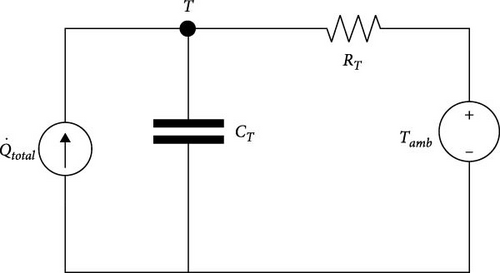
The battery thermal model can be simplified by dividing the battery into a thermal capacity and a thermal resistor. In Figure 1, T_amb represents the current ambient temperature, and R_T and C_T represent the overall thermal resistance and heat capacity, respectively. Assume that the overall material inside the battery is evenly distributed and that the parameters of all parts are the same. Therefore, based on Kirchhoff’s current law and Ohm’s law, the following relationship is established:

Details are in the caption following the image — **Figure 1**
Open in figure viewer PowerPoint

First-order thermal model.

(4)

In the first-order model, R_T and C_T, being difficult parameters to measure, usually need to be obtained by identification, so Equation (4) is rewritten as follows:

(5)

2.2. Second-Order TECM

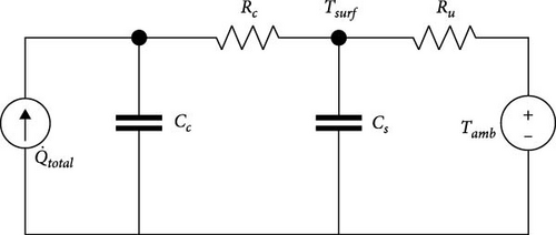
However, due to the different shapes and sizes of batteries, some batteries will have a large temperature difference between the core temperature and the surface temperature. Therefore, a second-order TECM was developed to represent two temperatures at different locations of the cell in terms of voltages at two different potentials.

In Figure 2, T_c and T_s represent the core temperature and surface temperature, respectively. The convective heat exchanges between the battery’s surface and the environment through the convective thermal resistance R_u. The heat exchanges between the core and surface through the conduction thermal resistance R_c. C_c and C_s denote the specific heat capacities of the core and surface of the battery, respectively. Here, it is assumed that the material inside the battery is uniform, implying a constant specific heat capacity at each position within the battery. The following relationship is established as follows:

(6)

Similar to the first-order TECM, the second-order TECM also requires the parameter values of R_u, R_c, and R_e to be determined by identification. Therefore, its Equation (6) is rewritten as follows:

(7)

Since the core temperature T_c is usually difficult to measure and obtain, its effect should be eliminated as much as possible during the identification process. Simplification of Equation (7) is as follows:

(8)

2.3. Parameter Identification of Thermal Model

Traditional parameter identification methods can be divided into offline identification and online identification. The offline identification method is to obtain the model parameters in advance for identification, and the online identification method is to use real-time data for identification. TECM needs to discuss its optimal identification method because it is closely related to the material properties of the battery, which is different from the EECM whose parameters change with the change of the working conditions. In this study, the more advanced adaptive weighting factor and forgetting factor recursive least squares (VWF-VFFRLS) [33] was chosen as the online identification method; meanwhile, the coyote optimization algorithm (COA) was chosen as a typical offline identification method. The two identification methods are used to identify the TECM parameters, respectively, and analyze the applicability and accuracy difference for TECM identification.

2.3.1. VWF-VFFRLS Identification Algorithm

According to Mao [33] based on the FFRLS method, VWF-VFFRLS introduces an adaptive method integrating the adjustment of variable forgetting factor and weighting factor, which realizes the fast-tracking of the current state of the system with the following:

(9)

where the K (k) denotes the gain of the parameter vector at time k-th iteration, P (k) is the error covariance matrix, θ is the parameter vector, and I is the unit matrix, λ is the forgetting factor, and Ɐ is the weighting factor. The following section briefly describes the identification process of first-order TECM and second-order TECM, respectively, using VWF-VFFRLS [34].

For the first-order thermal model, these methods align with the fundamental structure of the least square method fitting the equation y(k) = φ^T(k) × θ + e(k), facilitating the parameter estimation process, as given by the following:

(10)

(11)

The components of θ in the first-order thermal model identification process are as follows:

(12)

For the second-order model, according to the basic structure of the least square method, the following definitions are given as follows:

(13)

(14)

Among them, θ is composed as follows:

(15)

2.3.2. COA

COA is a bionic global optimization algorithm. Algorithm 1 draws inspiration from the life events of coyote populations, including birth, growth, death, and migration. The simplicity of implementation and fast convergence of COA make it widely used for parameter identification. For space reasons, the pseudocode for COA is listed in Table 1.

Table 1. Pseudocode of the COA [35].

Algorithm 1 Pseudocode of the COA.
1:	Initialize N_p packs with N_c coyotes each
2:	Verify the coyote’s adaptation.
3:	while the stopping criterion is not achieved do
4:	for each p pack do
5:	Define the alpha coyote of the pack
6:	Compute the social tendency of the pack
7:	for each c coyote of the p pack do
8:	Update the social condition
9:	Evaluate the new social condition
10:	Adaptation
11:	end for
12:	Selection of new individual parents。
13:	Compute the worse adapted group ω and the number of coyotes ϕ.
14:	ifϕ = 1 then
15:	The survives and the only coyote in ω dies.
16:	elseif ϕ > 1 then
17:	The survives and the oldest coyote in ω dies.
18:	Else
19:	The dies.
20:	end if
21:	end for
22:	Transition between packs
23:	Update the coyotes’ ages.
24:	end while
25:	Select the best adapted coyote

Abbreviation: COA, coyote optimization algorithm.

The table concludes the iterative process in COA. In the case of the TECM in this paper, the fitness function is defined as follows.

(16)

Similar to the process of online identification, after obtaining the corresponding battery data, the first-order thermal model and the second-order thermal model of the battery are identified offline. The following COA offline recognizes the first-order and second-order TECMs.

In the process of offline identification of the first-order thermal model parameters with COA, T (t) represents the real-time temperature of the battery, T_pre (t) represents the cell temperature calculated according to Equation (5). It is assumed that the target values C_T and R_T are known, thus iteratively. Denoting C_T and R_T in Equation (5) as the social status of individual mid-coyotes, the resulting COA algorithm can iterate over first-order thermal model parameters randomly generated over a set range, minimizing overall error by comparing predicted temperatures to experimentally obtained surface temperatures.

And in the offline identification process of the second-order thermal model parameters with COA, the data being identified are analogized to the social condition of a coyote individual in the COA, represented as . By comparing this calculated surface temperature with the measured temperature as Equation (8), a dataset minimizing the overall error is determined, aligning with the COA algorithm’s objective of minimizing this discrepancy. T_pre (t) can be replaced by Equation (8). It is similar to the iterative approach of the first-order thermal model, where the unknown parameters are iterated as if they were known quantities to obtain the optimal value.

3. TECM

By identifying and simulating the TECM, it is obtained that the temperature variation of the battery in TECM is a function of the heat generation Q and the internal resistance R_e. And the heat generation Q is also a function of the internal resistance R_e and the open-circuit voltage V_oc of the battery. Therefore, there are a large number of parameter interactions between the EECM and the TECM, and by using this feature, the values of the battery’s SOC, R_e, and other parameters can be obtained in the EECM as inputs to the TECM for obtaining the value of the heat generation Q. And the TECM feeds back the temperature T obtained through simulation into the EECM to correct its parameters in order to obtain a higher recognition accuracy. Therefore, the corresponding TEM model is established through the connection between the heat generation Q in the TECM and R_e and V_oc in the EECM, and the real-time simulation of the battery temperature T is realized through the operating state of the battery after obtaining the identification results of the overall model. In this paper, the structure of TEM with first-order TECM and second-order RC-EECM, for example, is shown in Figure 3.

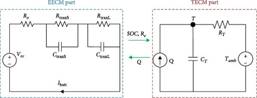
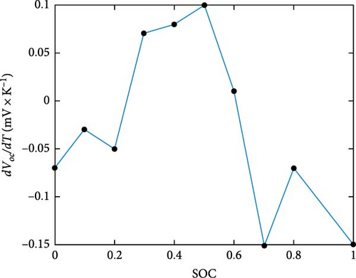
To calculate the amount of heat generation Q, it is first necessary to obtain the entropy heat coefficient dV_oc/dT and the internal resistance R_e in Equation (3). In TEM, the entropy heat coefficient dV_oc/dT can be considered as a function of SOC. By calculation, the relationship between entropy heat coefficient dV_oc/dT and SOC is shown in Figure 4. In addition, the internal resistance required in the heat calculation process can also be expressed as the sum of the EECM components R_o, R_tranS, and R_tranL. Therefore, the R_e parameter is obtained after selecting the VWF-VFFRLS to identify the EECM part of the TEM.

In addition, the SOC–V_oc curve is obtained by charging and discharging with small currents in a laboratory environment and then fitted with polynomials. Since a V_oc test is time-consuming and in [36] it was shown that the curve is less affected by the aging of the battery and does not change much during the whole life cycle, a new battery with SOH = 1 is chosen for fitting the SOC–V_oc curve. The resultant equation of the fitting is shown in Equation (17), where the parameters are all represented in Table 1. The SOC-VOCV relationship equation and specific parameters in the equation were derived through HPPC experiments and least squares fitting (given in Table 2).

Table 2. Fitting parameter.

Fitting result	p₁	p₂	p₃	p₄	p₅	p₆
Value	0.9215	−3.283	3.955	−1.248	0.2633	3.733

(17)

This value is one of the parameters of the heat generation of the thermal model, while the SOC is calculated by the CCM:

(18)

where SOC₀ is the initial SOC value of the battery and Q₀ is the initial capacity. In the following analysis, the discharging current is recorded as positive, while the charging current is recorded as negative. The flow of simulating the temperature of the battery by TEM is shown in Figure 5.

4. Model and Data-Driven Fusion Approach Modeling

4.1. Overview of the Fusion Approach Model

Based on the constructed TEM, the electrical characteristics and temperature variations of the battery are simulated under the condition that the battery operation data have been acquired. However, TEM-based temperature prediction methods are inevitably affected by small noise during the identification process or simulation. This noise makes the simulation results produce errors, especially when the battery is under complex operating conditions, and the effect of this noise will be further amplified. Therefore, in this section, the output of TEM is used as input to predict the temperature using a BiGRU-Transformer neural network based on KF optimization, to realize the temperature prediction method based on the fusion of model and data-driven in order to obtain the temperature prediction method with high accuracy and high adaptability.

To filter the parameters with higher correlation with the battery temperature as inputs, person correlation was used to evaluate the correlation of different parameters, and the results are shown in Figure 6. Heat generation Q, internal resistance R_e, battery current I, and battery voltage V were used as inputs to the data-driven part.

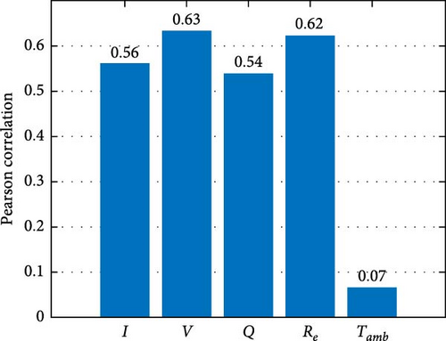
Furthermore, the correlation between the ambient temperature T_amb and the battery temperature change is low. However, the fact that the ambient temperature largely influences the baseline value of the battery temperature change, as well as the rate of temperature change of the battery, makes it one of the inputs to the data-driven model as well.

4.2. Relevant Theoretical Foundations

4.2.1. KF

KF acts as a recursive filter that is capable of estimating the state of a dynamic system from a series of incomplete and noise-containing measurements. In order to implement KF filtering, the model needs to be converted to be a spatial state model, which describes the development of the internal factors of the system and provides an expression for the relationship between the state values of the system and the observed values. The state transfer equations and the observation equations in KF are as follows:

(19)

where X_k and Y_k are the state vector and observation vector of the system at the moment k; u_k−1 is the input variable at the moment k-1; A, B, C, and D are the system matrix, control matrix, observation matrix, and feedforward matrix, respectively; and w (k) and v (k) are the system noise and observation noise, respectively.

The process of denoising the acquired signal using KF is divided into two steps: prediction and updating. The prediction process is as follows:

(20)

(21)

where

is the state at the previous moment;

is the state at the current moment; P_k−1 is the covariance at the previous moment;

is the a priori error covariance.

Then after the simple prediction based on the state equation, the observed states and gains in the KF need to be updated as follows:

(22)

(23)

(24)

where K_k is the Kalman gain; P_k is the posterior error covariance; and

is the posterior estimate.

By repeating the prediction and updating steps, the estimation of the system state is continuously optimized based on new measurements and the system model, and useful information is extracted from the noisy acquired signals, reducing the influence of noise on the signals.

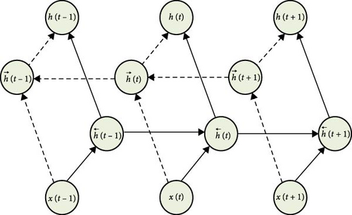
4.2.2. BiGRU Network

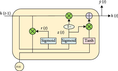
GRU is a variant of RNN designed to better handle long-term dependencies in sequential data and to prevent the gradient vanishing problem. The structure of GRU is given in Figure 7. Similar to LSTM, there are update gates and reset gates in GRU, which allow the network to selectively update the internal state. But the structure of GRU is simpler than that of LSTM, and GRU has the speed advantage of dealing with long time series data. The update gate and reset gate in GRU are represented as follows.

The reset gate controls the degree of influence of the past hidden state on the input of the current time step in GRU. By adjusting the output of the reset gate, the network can selectively forget the past information to flexibly handle the long-term dependencies in the sequence. The equation for the reset gate is as follows:

(25)

where r (t) is the output of the reset gate, σ is the sigmoid activation function, w_r and u_r are the corresponding weight matrices, x (t) is the input of the current time step, and h (t-1) is the past hidden state.

Update gate in GRU controls the extent to which the past hidden states are memorized for the current temporal input. By adjusting the output of the update gate, the network can selectively retain or forget the past information, thus adapting to different time series inputs. The equation of update gate is as follows:

(26)

where z (t) is the output of the reset gate and w_z and u_z are the corresponding weight matrices.

In GRU, the hidden state is always passed from front to back, which is not favorable to the feature extraction work. In the actual working state of the battery, the temperature changes in the front and back moments are highly correlated, and it is necessary to take such features into account. To extract the hidden features and complex changes in the time series by considering both before and after information, the GRU is structurally altered to obtain BiGRU. BiGRU consists of forward GRU and reverse GRU, and its hidden layer combines both forward and reverse information. In this way, BiGRU network can capture the before and after features in the time series information and increase the diversity of feature information. The hidden layer state h(t) of BiGRU at time t can be obtained by the state of the forward hidden layer

and the state of the reverse hidden layer

. The

is determined by the current input x (t) and the state of the forward hidden layer at time t−1, and the

is determined by the current input x (t) and the state of the backward hidden layer at time t + 1. BiGRU can be expressed as follows:

(27)

where w_i (i = 1,2,3…) denotes the corresponding weight of each layer. The structure of BiGRU is illustrated in Figure 8.

4.3. Transformer Network

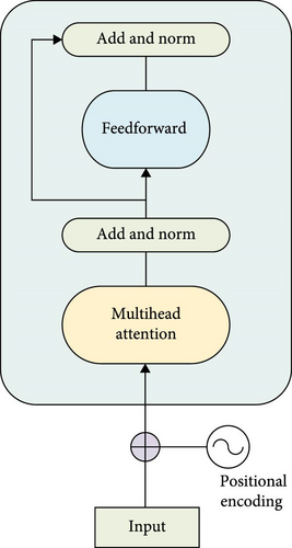
Transformer is a neural network architecture with superior performance. It is generally used in natural language processing, computer vision, time series prediction, etc. Its main feature is that it is based on attention mechanism rather than recursive structures (such as RNN and LSTM). A standard Transformer is a sequence-to-sequence architecture that consists of an encoder and a decoder. The encoder is responsible for mapping the input sequence into a vector of higher dimensions, which is then fed into the decoder to generate a series of outputs. Its conventional structure is shown in Figure 9.

The Transformer network needs to introduce positional coding to represent the positional information between the data in the sequence to enhance the generalization ability of the Transformer. And the calculation method of positional coding is expressed as follows:

(28)

(29)

where k denotes the sequence time step; u is the feature dimension of the input data sequence; and m is the length of the input sequence.

The Transformer network has two sublayers: the multihead self-attention mechanism layer and the feedforward layer. Among them, multiple self-attention improves the feature representation and prediction accuracy of the model by modeling the dependency of long sequences so that the model can focus on multiple regions at the same time, ignoring the distance between sequences, with the following expression:

(30)

(31)

where MultiHead denotes the multihead self-attention mechanism; Q, K, and V are the three vectors of the input sequence that have been linearly mapped; Contact is used to splice all the outputs of Head; W^o is the weight of the multiple attention; and Q_p, K_p, and V_p for Head of Q, K, and V corresponding to the weight matrix. Attention denotes the attention mechanism; the weight matrix is defined as shown as follows:

(32)

where d denotes the dimension of the vector.

The role of feedforward network (FFN) is to further extract features on the basis of the attention mechanism to enhance the expressive power of the model. FFN is denoted as follows:

(33)

where W₁ and W₂ denote the weights, b₁ and b₂ denote the biases, obtained by gradient descent training, and x denotes the input data.

4.4. KF-BiGRU-Transformer

In the timing prediction task, the raw data are affected by the acquisition process, and the result may be is not monotonous and smooth. These data are noisily processed by KF to reduce the effect of noise on the prediction and at the same time shorten the training time. BiGRU network can use its recursive property to extract the temporal features of the data, and the Transformer network can fully explore the global features of the data by modeling the data through the multihead self-attention mechanism and FFN switching. Therefore, this paper proposes a battery temperature prediction method (KF-BiGRU-Transformer) that combines KF, BiGRU, and Transformer. The method includes a data preprocessing module, a KF module, a BiGRU module, a Transformer module, and a fully connected (FC) module, as shown in Figure 10.

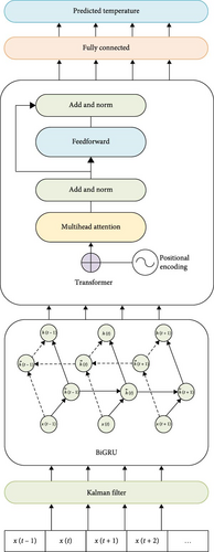
The modeling framework proposed in this paper can fully utilize the advantages of the Transformer network and KF: In the process of collecting battery data, the sensor or transmission process will inevitably be affected by noise. Therefore, reducing the noise in the data before adding the KF to the BiGRU network will reduce some of the prediction arithmetic burden while enhancing the subsequent prediction accuracy and reducing the impact of noise. The equations of state and the spatial equations of the KF are established based on the TEM and perform the noise reduction process on the data acquired from the experiments. Next, the processed time series are fed into the BiGRU module, which consists of two single-layer BiGRU networks, respectively. In this case, each single-layer BiGRU passes its output to the next layer after processing by an activation function, so that each layer can learn information at different time scales. This structure helps to better capture the long-term dependencies between battery temperature and other parameters in long sequences, thus improving the information extraction ability of the model. And then, the attentional weights of the multiattention mechanism can better integrate the uncertainty information in the battery temperature data and focus on the parameter (current, voltage, heat generation, etc.) effects on the battery temperature to improve the prediction accuracy. Therefore, the features extracted from the BiGRU module are input into the Transformer module, and the data features at different locations are extracted and spliced using the multihead attention mechanism and then nonlinearly transformed through the FFN. Finally, the output of the Transformer is input into the FC layer for real-time prediction of the battery temperature. In summary, the strategy adopted in this paper can maximize the advantages of the KF, BiGRU, and Transformer network to achieve good prediction results.

4.5. Fusion Method Prediction Process

Based on the above TEM and KF-BiGRU-Transformer theories, the flow of the hybrid model and data-driven modeling approach proposed in this paper is shown in Figure 11, which includes three basic parts, that is, obtaining parameter identification of the TEM, training of the data-driven model, and testing.

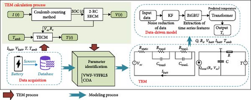
First, the actual operating parameters of the battery are obtained through various types of sensors, including the voltage, current, and surface temperature of the battery as well as the ambient temperature. Then, based on the results of online and offline identification for different TECMs, the identification method with relatively higher accuracy is selected to identify the parameters of the TECMs in the TEM, and the VWF-VFFRLS is used to identify the parameters of the EECMs in the TEM. The TEM can accurately describe the dynamic temperature change during the battery operation and provide the variation of electrical characteristics of different chemical reactions inside the battery. In addition, to prevent errors in the identification results in the modeling part from affecting the results of the neural network model, the accuracy of the model is calculated by simulation before neural network training is carried out.

Second, the TEM model is used to simulate the simulation to obtain the values of some parameters that cannot be obtained by the sensors, such as the amount of heat generated Q and the internal resistance of the battery R_e. Then, all recorded datasets and parameters with high correlation were obtained, and the input dataset was obtained by Pearson correlation coefficient method. The interaction between the TEM and the data-driven part is realized by this method of using the data simulated by the TEM and the actual sampled data as inputs to the KF-BiGRU-Transformer part.

Third, a neural network-based data-driven model is developed, which consists of KF to optimize the input data, BiGRU for feature extraction in the time series, and finally Transformer for temperature prediction. The model is trained using the parameters selected in Figure 6, which takes the heat generation Q, internal resistance R_e, current of battery I_batt, voltage of the battery V_batt, and ambient temperature T_amb as inputs and the battery temperature T as output.

Finally, based on the training and validation results, the proposed model successfully realizes the online prediction of battery temperature based on the hybrid model.

In this way, the proposed model and the data-driven hybrid model cannot only have real-time high-precision prediction, but also bypass the huge arithmetic power of real-time simulation of the TEM model.

5. Experiment Validation

As shown in Figure 12, constant temperature charging and discharging experiments were carried out on two Pokefi SY300-1 Li-polymer batteries, where the nominal capacity of Pokefi SY300-1 was converted to an equivalent capacitance of 13860 F. Among them, Bat1 was a new battery with SOH value of 1 and Bat2 with SOH values of 0.6578, where the voltage, current, and surface temperature of the cells were recorded by a Hioki LR8450 data logger.

5.1. Experimental Data Analysis

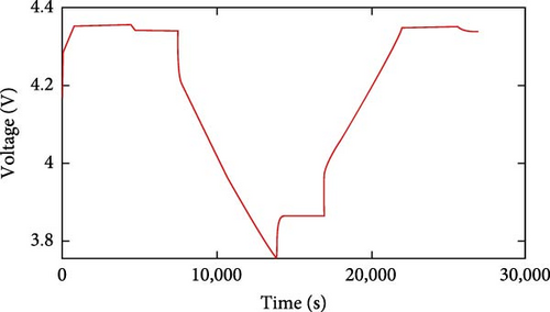
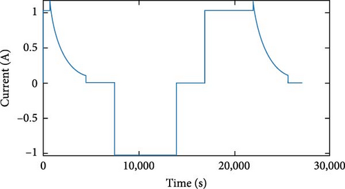
Validate the accuracy of the proposed TEM for Li batteries as well as obtain inputs for the neural network model through a series of experiments. Online and offline identification methods for determining the parameters of the battery thermal model were evaluated using complete charge and discharge data. Two batteries Bat1 and Bat2 with different SOH were selected for the experiment. The batteries all went through three stages of discharge, resting, and charging during the experimental operation. The measured output voltages and currents of the two batteries are shown in Figure 13. The charging current was set to be positive, and the discharging current was set to be negative.

In the experiment, the surface temperature and ambient temperature of the two batteries were monitored and recorded separately, as shown in Figure 14. The laboratory temperatures were all maintained at approximately 34.7°C for the experiment. Initially, both Bat1 and Bat2 showed a small increase in battery surface temperature during the short charging phase at the beginning of the experiment. Subsequently, the surface temperatures of both batteries decreased rapidly during the resting period but eventually stabilized. And then again, during the constant current discharge phase, the batteries warmed up rapidly. At the same time, its surface temperature remains high. When the battery is discharged to the lowest operating voltage, the discharge stops. Then, a rapid decrease in the surface temperature of the battery can be observed. Subsequently, constant current charging begins. The maximum surface temperature in this stage is 35.6°C, which is lower than the temperature in the discharge stage.

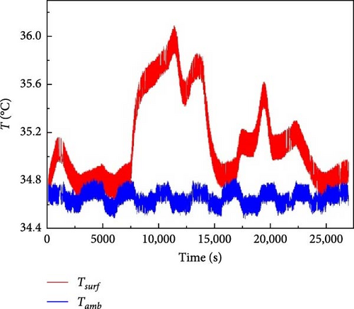
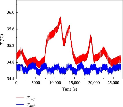
The EECM model, as part of the TEM, has the main role of providing the TECM part with the internal resistance R_e and the open-circuit voltage V_oc. Conversely, the temperature predicted by the TECM part also reacts back to the EECM for parameter correction. However, this paper focuses more on the parametric inputs from the EECM to the TECM. Therefore, the EECM needs to use VWF-VFFRLS identification to obtain the internal resistance of the battery R_e. In the model proposed in this paper, the internal resistance R_e is the sum of all the resistance values in the EECM model, and the identification results are shown in Figure 15.

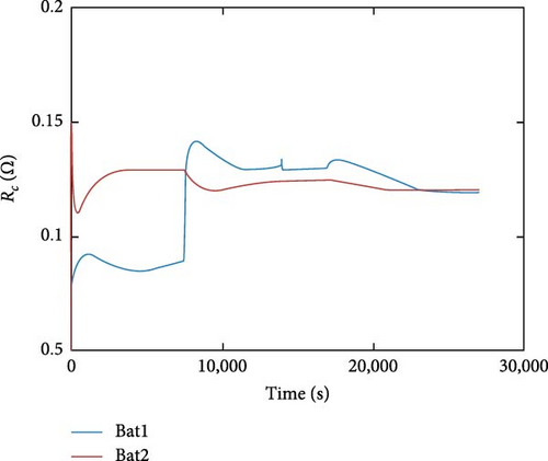
The trend of the internal resistance R_e of Bat1 and Bat2 with the charging and discharging process can be seen from Figure 15. As can be seen from Figure 15, the internal resistance of both batteries experienced a rapid rise at the beginning and then stabilized, but the internal resistance of Bat1 showed significant fluctuations after about 10,000 s, while the internal resistance of Bat2 was relatively smooth. This variation in internal resistance may affect the accuracy of the battery temperature prediction, and although the small value of the internal resistance R_e is analyzed from a mathematical point of view and its effect on the temperature estimation does not cause an excessive shift in the results, it seriously affects the goal of high accuracy of the prediction. Therefore, in practice, the dynamic changes in internal resistance need to be considered, especially for Bat1, whose fluctuations in internal resistance may require special attention and adjustment of model parameters to accurately predict temperature changes.

5.2. Validation of Thermal Model Identification

For the offline identification of the first-order thermal model with COA, the parameter settings of the algorithm are as follows: 50 coyote individuals are utilized, and the algorithm undergoes a total of 200 iterations. The iteration range for thermal resistance is defined as (0, 100), while the iteration range for heat capacity is set between (0, 1000). After iterations, the thermal resistance of the cell in the first-order thermal model is computed as 4.0619 K/W⁻¹, and the heat capacity is determined to be 411.3769 J/K⁻¹. At the same time, the obtained battery data are identified online by VWF-VFFRLS. To demonstrate the accuracy of VWF-VFFRLS in online identification, the simplest FFRLS is also validated here.

The first-order thermal model parameters obtained by the on-line and off-line identification methods mentioned in Section 2 are simulated and verified, respectively. The simulated temperatures resulting from these parameter sets were compared with the actual battery temperatures, as illustrated in Figure 16. It can be observed that, for the first-order thermal model, the simulated temperature changes of the battery derived from the three methods closely align with the actual temperature variations. The temperature error differences among the three methods are relatively minor. This similarity in the error values can be attributed to the simplicity of the first-order model, where many algorithms exhibit comparable accuracy due to the model’s straightforward nature.

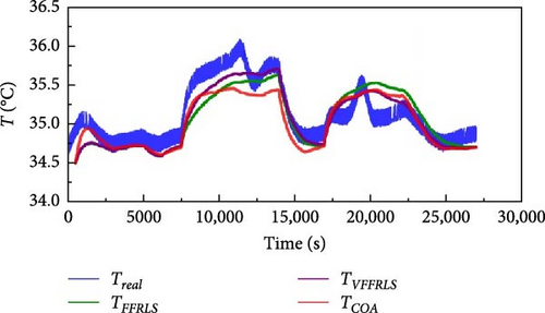
Similar to the identification process of the first-order thermal model, the offline identification parameters of the second-order thermal model are set as follows: The iteration range for thermal resistance is set as (0, 100), and the iteration range for heat capacity is specified as (0, 2000). The second-order TECM part is identified and iterated by the COA algorithm, and the heat capacity of the core C_c and the heat capacity of the surface C_s in the thermal model are obtained to be 64.973 J/K⁻¹ and 4.649 J/K⁻¹, respectively, whereas the conduction thermal resistance R_c and the convection thermal resistance R_u are obtained to be 2.989 K/W⁻¹ and 3.4817 K/W⁻¹, respectively. At the same time, the obtained battery data are identified online by FFRLS and VWF-VFFRLS, respectively.

The simulated temperatures of the second-order thermal model and the actual measured surface temperatures of the cell obtained by different algorithmic identification are shown in Figure 17. It is found that the error by online identification approach is larger than that by offline identification method. In order to assess the accuracy of temperature prediction from different identification methods, the RMSE is used as an evaluation metric. RMSE is denoted as follows:

(34)

where T_real is the real temperature, T_sim denotes the simulated or predicted temperature, and n denotes the number of sampled values.

By calculating the RMSE of the simulated temperatures of the different identification methods in the TECM section, it is found that the RMSE of the COA algorithm as an offline identification algorithm is only 0.2156, which is much lower than that of the FFRLS at 0.2512 and the VWF-VFFRLS at 0.2441. This enhanced accuracy can be attributed to the stability of the battery’s material properties. Despite potential chemical changes during battery usage, the material properties remain relatively constant. Therefore, the heat capacity of the battery material appears more consistent when incorporated into the thermal model [37]:

(35)

where L signifies the thickness of the thermally conductive material, S represents the contact area, and k’ corresponds to the thermal conductivity. The values of L and S are fixed in the same battery model. The value of R_T is determined by the properties of the different materials in the battery, and since the properties of these materials usually change very little in most of the experiments, it is more reasonable to set the value of the thermal resistance of the battery as a constant value.

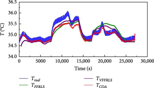
After obtaining the parameters of the thermal model of the battery, the TEM developed in Section 3 can be verified. Based on the internal resistance R_e of the battery obtained from the identification, the heat generation of the battery can also be derived from Equation (3). Therefore, the corresponding model is built in MATLAB/Simulink, and the voltage following and temperature following of the two batteries are compared to verify the accuracy of the model. The RMSE calculations of the two batteries and their results are shown in Table 3. The RMSE of the TEM is expressed as the average value of the RMSE of the voltage verification results in the electrical model part and the temperature verification results in the thermal model part.

Table 3. RMSE of battery TEM.

Battery number	RMSE
Bat1	0.2198
Bat2	0.2759

Abbreviations: RMSE, root mean square error; TEM, thermoelectric equivalent model.

From the validation results of the thermoelectric model, it can be seen that the accuracy of the model can already track the actual accuracy well. However, in practical applications, it is impossible to eliminate the ineliminable oscillations brought about by VWF-VFFRLS at the beginning of the partial identification process of the electrical model, which largely affects the accuracy of the model. Therefore, based on the thermal model, combined with the data-driven algorithm, real-time prediction of the temperature of the thermal model can be realized, thus greatly avoiding this error.

5.3. Validation of KF-BiGRU-Transformer to Predict Battery Temperature

For temperature prediction, two batteries with different SOH were selected for the study. The charging and discharging processes of the first brand new battery Bat1 and the second battery with SOH value of 0.6578 Bat2 are exactly the same. Initially, voltage, current, and ambient temperature data from the two cells, as well as computationally acquired heat generation and internal resistance, were used as inputs, and the surface temperature of each cell was used as an output. Bat1 is the training set when Bat2 is the prediction set at this point.

In the experiments, CNN, GRU, LSTM, BiGRU, and SSA-LSTM are set as control groups, where the hyperparameters of CNN, GRU, LSTM, and BiGRU models are the same as those of KF-BiGRU-Transformer. And the hyperparameters of SSA-LSTM model are optimized by SSA. Based on the RMSE comparison, the training effect of KF-BiGRU-Transformer is significantly better than other neural networks. Therefore, the data of Bat1 are firstly trained as the training set, and the obtained training results are shown in Figure 18 and Table 4. It can be seen that the RMSE of KF-BiGRU-Transformer on Bat1 data is only 0.0570, which is much smaller than the remaining four control sets. This indicates that the KF-BiGRU-Transformer is trained with extremely high accuracy under the same training conditions and can have better results in the subsequent tests.

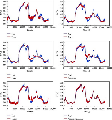
Table 4. Comparison of errors in prediction methods.

Method	Average error (%)	Maximum error (°C)	RMSE (°C)
Training set
CNN	0.18361	0.68139	0.0945
GRU	0.20813	0.75062	0.1113
LSTM	0.25172	0.76128	0.1290
BiGRU	0.20888	0.50976	0.1066
SSA-LSTM	0.26767	0.65737	0.1437
KF-BiGRU-Transformer	0.1194	0.28054	0.0570
Test set
CNN	0.10733	0.5247	0.14758
GRU	0.1056	0.68429	0.14845
LSTM	0.12364	0.63383	0.16458
BiGRU	0.1140	0.4396	0.1494
SSA-LSTM	0.12427	0.44457	0.14095
KF-BiGRU-Transformer	0.10418	0.3423	0.1266

Abbreviations: GRU, gated recurrent unit; KF, Kalman filter; LSTM, long short-term memory; RMSE, root mean square error; SSA, sparrow search algorithm.

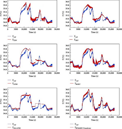
The results with Bat2 used for testing are shown in Figure 19 and Table 4, and the KF-BiGRU-Transformer proposed in this paper predicts the temperature results of Bat2 with an RMSE of 0.1266, which is better than the other five sets of neural networks. However, it can be observed that there is still a relative error in the fitting of the test results on the battery peak, which is mainly caused by the influence of the training data. However, the maximum prediction error of the model in Bat2 is 0.3423°C. This peak error is acceptable for temperature prediction, and the prediction accuracy will be further improved if there exist more training results under more working conditions. In addition, the average prediction error of the model in Bat2 is 0.10418°C, which indicates that the KF-BiGRU-Transformer model is more effective in predicting the battery temperature process under the complete working conditions and also indicates that the model can also predict the temperature well under different SOH conditions.

6. Conclusions

This paper presents a modeling and data-driven fusion approach to predict battery temperature. The method first analyzes the first-order and second-order TECM of the battery, aiming to help related research to select the most suitable TECM for battery temperature prediction. For the first-order TECM, no significant differences were found between the online method (VWF-VFFRLS) and the offline identification (COA). For the second-order TECM, the offline identification method using COA is significantly more accurate. Subsequently, a TEM combining EECM and TECM was proposed. However, it was found that the model-based approach required higher computational resources during computation, and parameter oscillations interfered with the identification results during the initial stage of identifying certain parameters. Therefore, in this study, a combined modeling and data-driven temperature prediction method is proposed for batteries under different SOH conditions. KF-BiGRU-Transformer is utilized as the data-driven part, firstly, KF is utilized to perform noise reduction on the collected data, then BiGRU is utilized to extract the characteristics of temporal relationship between the data with respect to sensitivities in the time series, and finally, Transformer is utilized to extract the characteristics of the data at different locations for temperature prediction. Validation of the proposed hybrid model reveals that its average temperature error can be controlled at 0.29%, and the prediction errors RMSE are 0.0570 and 0.1266 for two types of batteries under different SOH, respectively. The results show that the estimation method is not only highly accurate, but also has a good generalization to batteries under different SOH conditions

Theoretically, the modeling approach in this paper is general, and the TECM in the TEM can be substituted for the first- and second-orders according to the actual situation. Similarly, the EECM can be replaced according to the specific working conditions. This makes the model suitable for temperature estimation studies of different models of Li-ion batteries under different operating conditions, and only the model parameters need to be adjusted according to the specific battery. In order to improve the generality and temperature estimation accuracy of the fusion model, in the subsequent research, on the one hand, the data-driven part is optimized, and the network structure is improved, so that the data-driven model can be trained to modify the model parameters by obtaining a small amount of new battery data to improve the training efficiency; moreover, the applicability of changing the prediction model under different room temperatures will be considered in the subsequent research work, and the corresponding corrections will be made, and on the other hand, the balance between the computational complexity of the thermoelectric model and the simulation accuracy needs to be addressed.

Nomenclature

:: Heat generation rate
Vol:: Volume of the battery (m³)
V_batt:: Voltage of the battery (V)
V_oc:: Open-circuit voltage (V)
dV_oc/dT:: Entropy change coefficient
T:: Battery temperature (°C)
I_batt:: Current of the battery (A)
R_p:: Polarization resistance (Ω)
R_o:: Ohmic internal resistance (Ω)
R_e:: Internal resistance (Ω)
T_amb:: Current ambient temperature (°C)
R_T:: Thermal resistance (K/W⁻¹)
C_T:: Heat capacity (J/K⁻¹)
T_c:: Core temperature (°C)
T_s:: Surface temperature (°C)
C_c:: Heat capacity of the core (J/K⁻¹)
C_s:: Heat capacity of the surface (J/K⁻¹)
R_u:: Convection thermal resistance (K/W⁻¹)
R_c:: Conduction thermal resistance (K/W⁻¹)
λ:: Forgetting factor
Ɐ:: Weighting factor
N_p:: Population size
N_c:: Number of individuals
:: Social condition of a coyote individual
:: Coyote’s adaptation
lead^p,t:: Alpha coyote of the pack
:: Social tendency of the pack
:: New individual parents
ω:: Worse adapted pack
ϕ:: Number of coyotes
P_c:: Transition between packs
R_tranS, R_tranL:: Polarization resistances (Ω).

Glossary

BMSs:: Battery management systems
DCFC:: DC fast charging
EECM:: Electrical equivalent circuit model
EKF:: Extended Kalman filter
ETNN:: Electrochemical–thermal neural network
EV(s):: Electric vehicle(s)
FRA:: Fast recursive algorithm
GRU:: Gated recurrent unit
LSTM:: Long short-term memory
OCV:: Open-circuit voltage
PINN:: Physically informed neural network
RNN:: Recurrent neural network
SOC:: State of charge
SOH:: State of health
SOT:: State of temperature
SSA:: Sparrow search algorithm
TECM:: Thermal equivalent circuit modeling
TEM:: Thermoelectric equivalent model
TSM:: Two-state thermal model
UKF:: Untraceable Kalman filtering.

Conflicts of Interest

The authors declare no conflicts of interest.

Funding

This work was supported by the Ministry of Education (MoE) Academic Research Fund (AcRF) Tier-1 Seed Fund RS12/23 and the Major Science and Technology Projects in Zhejiang Province – Key R&D Projects (2023C01SA301767).

Acknowledgments

Open Research

Data Availability Statement

The data supporting this study’s findings are available from the corresponding author upon reasonable request.

References

1 Xie J. and Lu Y.-C., A Retrospective on Lithium-Ion Batteries, Nature Communications. (2020) 11, no. 1, https://doi.org/10.1038/s41467-020-16259-9, 2499.
10.1038/s41467-020-16259-9
CAS PubMed Web of Science® Google Scholar
2 Zhang G., “Revealing the Impact of Slight Electrical Abuse on the Thermal Safety Characteristics for Lithium-Ion Batteries, ACS Applied Energy Materials, 2021, 4, no. 11, 12858–12870.
Google Scholar
3 Zhou Z., Li M., and Zhou X., Investigating Thermal Runaway Triggering Mechanism of the Prismatic Lithium Iron Phosphate Battery Under Thermal Abuse, Renewable Energy. (2024) 220, https://doi.org/10.1016/j.renene.2023.119674, 119674.
10.1016/j.renene.2023.119674
Web of Science® Google Scholar
4 Xing B., Xiao F., Korogi Y., Ishimaru T., and Xia Y., Direction-Dependent Mechanical-Electrical-Thermal Responses of Large-Format Prismatic Li-Ion Battery Under Mechanical Abuse, Journal of Energy Storage. (2021) 43, https://doi.org/10.1016/j.est.2021.103270, 103270.
10.1016/j.est.2021.103270
Web of Science® Google Scholar
5 Richardson R. R., Ireland P. T., and Howey D. A., Battery Internal Temperature Estimation by Combined Impedance and Surface Temperature Measurement, Journal of Power Sources. (2014) 265, 254–261, https://doi.org/10.1016/j.jpowsour.2014.04.129, 2-s2.0-84901284565.
10.1016/j.jpowsour.2014.04.129
CAS Web of Science® Google Scholar
6 Tang R., Zhang P., Ning S., and Zhang Y., Prediction of Battery SOH and RUL Based on Cooperative Characteristics in Voltage-Temperature-Time Dimensions, Journal of The Electrochemical Society. (2023) 170, no. 6, https://doi.org/10.1149/1945-7111/acde10, 060535.
10.1149/1945-7111/acde10
CAS Web of Science® Google Scholar
7 Yue X., Fu Q., Hu H., and Wang D., Hammerstein Model Based Battery SOC Estimation Considering Temperature Variation, Journal of The Electrochemical Society. (2024) 171, no. 3, https://doi.org/10.1149/1945-7111/ad2d8e, 030503.
10.1149/1945-7111/ad2d8e
CAS Web of Science® Google Scholar
8 Yang Y., Tan S.-C., and Hui S. Y. R., State-of-Charge Balance Control of Distributed Battery Systems With Distinct State-of-Health in DC Microgrids, 2021 IEEE/IAS Industrial and Commercial Power System, 2021, Asia, Chengdu, China.
Google Scholar
9 Yang J., Cai Y., and Mi C., Lithium-Ion Battery Capacity Estimation Based on Battery Surface Temperature Change Under Constant-Current Charge Scenario, Energy. (2022) 241, https://doi.org/10.1016/j.energy.2021.122879, 122879.
10.1016/j.energy.2021.122879
Web of Science® Google Scholar
10 Manas M., Yadav R., and Dubey R. K., Designing a Battery Management System for Electric Vehicles: A Congregated Approach, Journal of Energy Storage, 2023, 74, 109439.
Google Scholar
11 Liang H.-W. R., Yang Y., and Hui S. Y. R., Improvement of Lithium-Ion Battery Charging From the State-of-the-Art Industrial JEITA Guidelines to a Hybrid Temperature-Regulated Current Control, IEEE Transactions on Power Electronics. (2022) 37, no. 6, 6412–6423, https://doi.org/10.1109/TPEL.2021.3133605.
10.1109/TPEL.2021.3133605
Web of Science® Google Scholar
12 Cwiok K., Develeopment, Characterization & Implementation of Phase-Change Material Cold Plates for Hybrid-Electric Vehicle Battery Systems, 2016, Embry-Riddle Aeronautical University, M. S. thesis.
Google Scholar
13 Srinivasan V. and Wang C. Y., Analysis of Electrochemical and Thermal Behavior of Li-Ion Cells, Journal of the Electrochemical Society. (2002) 150.
Google Scholar
14 Bernardi D., Pawlikowski E., and Newman J., A General Energy Balance for Battery Systems, Journal of the Electrochemical Society. (1985) 132, no. 1, 5–12, https://doi.org/10.1149/1.2113792, 2-s2.0-0021850417.
10.1149/1.2113792
CAS Web of Science® Google Scholar
15 Zhoujian A., Investigation on Lithium-Ion Battery Electrochemical and Thermal Characteristic Based on Electrochemical-Thermal Coupled Model, Applied Thermal Engineering, 2018, 137, 792–807.
Google Scholar
16 Chiew J., Chin C. S., Toh W. D., Gao Z., Jia J., and Zhang C. Z., A Pseudo Three-Dimensional Electrochemical-Thermal Model of a Cylindrical LiFePO4/Graphite Battery, Applied Thermal Engineering. (2019) 147, 450–463, https://doi.org/10.1016/j.applthermaleng.2018.10.108, 2-s2.0-85055580943.
10.1016/j.applthermaleng.2018.10.108
CAS Web of Science® Google Scholar
17 Surya S., Marcis V., and Williamson S., Core Temperature Estimation for a Lithium Ion 18650 Cell, Energies. (2021) 14.
Web of Science® Google Scholar
18 Lin X., Perez H. E., and Siegel J. B., et al.Online Parameterization of Lumped Thermal Dynamics in Cylindrical Lithium Ion Batteries for Core Temperature Estimation and Health Monitoring, IEEE Transactions on Control Systems Technology. (2013) 21, no. 5, 1745–1755, https://doi.org/10.1109/TCST.2012.2217143, 2-s2.0-84897584082.
10.1109/TCST.2012.2217143
Web of Science® Google Scholar
19 Pang H., Guo L., Wu L., Jin J., Zhang F., and Liu K., A Novel Extended Kalman Filter-Based Battery Internal and Surface Temperature Estimation Based on an Improved Electro-Thermal Model, Journal of Energy Storage. (2021) 41, https://doi.org/10.1016/j.est.2021.102854, 102854.
10.1016/j.est.2021.102854
Web of Science® Google Scholar
20 Saqli K., Bouchareb H., M’sirdi N. K., and Oudghiri Bentaie M., Lithium-Ion Battery Electro-Thermal Modelling and Internal States Co-Estimation for Electric Vehicles, Journal of Energy Storage. (2023) 63, https://doi.org/10.1016/j.est.2023.107072, 107072.
10.1016/j.est.2023.107072
Web of Science® Google Scholar
21 Chen L., Hu M., Cao K., Li S., Su Z., Jin G., and Fu C., Core Temperature Estimation Based on Electro-Thermal Model of Lithium-Ion Batteries, International Journal of Energy Research. (2020) 44, no. 7, 5320–5333, https://doi.org/10.1002/er.5281.
10.1002/er.5281
CAS Web of Science® Google Scholar
22 Liu Z. and Li H.-X., A Spatiotemporal Estimation Method for Temperature Distribution in Lithium-Ion Batteries, IEEE Transactions on Industrial Informatics. (2014) 10, no. 4, 2300–2307, https://doi.org/10.1109/TII.2014.2341955, 2-s2.0-84910096328.
10.1109/TII.2014.2341955
Web of Science® Google Scholar
23 Jiang Y. H., Yu Y. F., Huang J. Q., Cai W. W., and Marco J., Li-Ion Battery Temperature Estimation Based on Recurrent Neural Networks, Science China Technological Sciences. (2021) 64, no. 6, 1335–1344, https://doi.org/10.1007/s11431-020-1736-5.
10.1007/s11431-020-1736-5
CAS Web of Science® Google Scholar
24 Yao Q., Lu D. D.-C., and Lei G., A Surface Temperature Estimation Method for Lithium-Ion Battery Using Enhanced GRU-RNN, IEEE Transactions on Transportation Electrification. (2023) 9, no. 1, 1103–1112, https://doi.org/10.1109/TTE.2022.3197927.
10.1109/TTE.2022.3197927
Web of Science® Google Scholar
25 Cho G., Zhu D., Campbell J. J., and Wang M., An LSTM-PINN Hybrid Method to Estimate Lithium-Ion Battery Pack Temperature, IEEE Access. (2022) 10, 100594–100604, https://doi.org/10.1109/ACCESS.2022.3208103.
10.1109/ACCESS.2022.3208103
Web of Science® Google Scholar
26 Liu Y., Huang Z., Wu Y., Yan L., Jiang F., and Peng J., An Online Hybrid Estimation Method for Core Temperature of Lithium-Ion Battery With Model Noise Compensation, Applied Energy. (2022) 327, https://doi.org/10.1016/j.apenergy.2022.120037, 120037.
10.1016/j.apenergy.2022.120037
Web of Science® Google Scholar
27 Liu K., Li K., and Deng J., A Novel Hybrid Data-Driven Method for Li-Ion Battery Internal Temperature Estimation, 11th International Conference on Control (CONTROL), 2016, Belfast, UK, IEEE, 1–6, https://doi.org/10.1109/CONTROL.2016.7737560, 2-s2.0-85003845895.
10.1109/CONTROL.2016.7737560
Google Scholar
28 Feng F., Teng S., Liu K., Xie J., Xie Y., Liu B., and Li K., Co-Estimation of Lithium-Ion Battery State of Charge and State of Temperature Based on a Hybrid Electrochemical-Thermal-Neural-Network Model, Journal of Power Sources. (2020) 455, https://doi.org/10.1016/j.jpowsour.2020.227935, 455.
10.1016/j.jpowsour.2020.227935
Web of Science® Google Scholar
29 Yao F., Remaining Useful Life Prediction of Lithium-Ion Batteries Using a Hybrid Model, Energy, 2022, 248, 123622.
Google Scholar
30 Zhang Y., Peng Z., Guan Y., and Wu L., Prognostics of Battery Cycle Life in the Early-Cycle Stage Based on Hybrid Model, Energy. (2021) 221, https://doi.org/10.1016/j.energy.2021.119901, 119901.
10.1016/j.energy.2021.119901
Web of Science® Google Scholar
31 Chen X.-D., Yang H.-Y., Wun J.-S., Wang C.-H., and Li L.-L., Life Prediction of Lithium-Ion Battery Based on a Hybrid Model, Energy Exploration & Exploitation. (2020) 38, no. 5, 1854–1878, https://doi.org/10.1177/0144598720911724.
10.1177/0144598720911724
CAS Web of Science® Google Scholar
32 Talluri T., Murugesan S., and Karthikeyan V., the Capacity Estimation of Li-Ion Battery Using ML-Based Hybrid Model, Electrical Engineering, 2024.
Google Scholar
33 Mao Y., Bao J., Zhang Y., and Yang Y., An Ultrafast Variable Forgetting Factor Recursive Least Square Method for Determining the State-of-Health of Li-Ion Batteries, IEEE Access. (2023) 11, 141152–141161, https://doi.org/10.1109/ACCESS.2023.3340631.
10.1109/ACCESS.2023.3340631
Web of Science® Google Scholar
34 Mao Y., Bao J., Zhang Y., and Yang Y., An Ultrafast State-of-Health Monitoring Scheme for Li-ion Batteries Based on A Simple Electrical Model, 2023 IEEE Transportation Electrification Conference and Expo, Asia-Pacific, Chiang Mai, Thailand, 2023, ITEC.
Google Scholar
35 Pierezan J. and Coelho L. Dos Santos, Coyote Optimization Algorithm: A New Metaheuristic for Global Optimization Problems,” 2018, 2018, IEEE Congress on Evolutionary Computation, Rio de Janeiro, Brazil.
Google Scholar
36 Abu-Sharkh S. and Doerffel D., Rapid Test and Non-Linear Model Characterisation of Solid-State Lithium-Ion Batteries, Journal of Power Sources. (2004) 130, no. 1-2, 266–274, https://doi.org/10.1016/j.jpowsour.2003.12.001, 2-s2.0-1842421801.
10.1016/j.jpowsour.2003.12.001
CAS Web of Science® Google Scholar
37 Dong T., Peng P., and Jiang F., Numerical Modelling and Analysis of the Thermal Behavior of NCM Lithium-Ion Batteries Subjected to Very High C-Rate Discharge/Charge Operations, International Journal of Heat and Mass Transfer. (2018) 117, 261–272, https://doi.org/10.1016/j.ijheatmasstransfer.2017.10.024, 2-s2.0-85031024836.
10.1016/j.ijheatmasstransfer.2017.10.024
CAS Web of Science® Google Scholar

All articles

A Data-Driven-Aided Thermoelectric Equivalent Circuit Model for Accurate Temperature Prediction of Lithium-Ion Batteries

Abstract

1. Introduction

2. TECM and Parameter Identification

2.1. First-Order TECM

2.2. Second-Order TECM

2.3. Parameter Identification of Thermal Model

2.3.1. VWF-VFFRLS Identification Algorithm

2.3.2. COA

3. TECM

4. Model and Data-Driven Fusion Approach Modeling

4.1. Overview of the Fusion Approach Model

4.2. Relevant Theoretical Foundations

4.2.1. KF

4.2.2. BiGRU Network

4.3. Transformer Network

4.4. KF-BiGRU-Transformer

4.5. Fusion Method Prediction Process

5. Experiment Validation

5.1. Experimental Data Analysis

5.2. Validation of Thermal Model Identification

5.3. Validation of KF-BiGRU-Transformer to Predict Battery Temperature

6. Conclusions

Nomenclature

Glossary

Conflicts of Interest

Funding

Acknowledgments

Open Research

Data Availability Statement

References

Figures

References

Information

About Wiley Online Library

Help & Support

Opportunities

Connect with Wiley

A Data-Driven-Aided Thermoelectric Equivalent Circuit Model for Accurate Temperature Prediction of Lithium-Ion Batteries

Abstract

1. Introduction

2. TECM and Parameter Identification

2.1. First-Order TECM

2.2. Second-Order TECM

2.3. Parameter Identification of Thermal Model

2.3.1. VWF-VFFRLS Identification Algorithm

2.3.2. COA

3. TECM

4. Model and Data-Driven Fusion Approach Modeling

4.1. Overview of the Fusion Approach Model

4.2. Relevant Theoretical Foundations

4.2.1. KF

4.2.2. BiGRU Network

4.3. Transformer Network

4.4. KF-BiGRU-Transformer

4.5. Fusion Method Prediction Process

5. Experiment Validation

5.1. Experimental Data Analysis

5.2. Validation of Thermal Model Identification

5.3. Validation of KF-BiGRU-Transformer to Predict Battery Temperature

6. Conclusions

Nomenclature

Glossary

Conflicts of Interest

Funding

Acknowledgments

Open Research

Data Availability Statement

References

Figures

References

Related

Information