1. Introduction

Lithium-ion battery (LIB) has a high energy density, a low self-discharge rate, and high performance compared to other battery types [1, 2]. These characteristics make them widely used in a variety of fields, including military, transportation, and aerospace, where high power output and long run times are required [3–5]. The internal resistance of LIBs increases with repeated use due to irreversible chemical reactions. According to the research results of Ko et al. [6], abnormal situations such as collision and misuse are reported to promote internal damage to the battery, causing a rapid increase in internal resistance.

An increase in internal resistance means that the battery is aging and indicates that permanent capacity loss has occurred. Therefore, permanent capacity loss means that the maximum available capacity has decreased, which leads to a decrease in the performance of the battery, such as maximum power output and runtime [7]. Therefore, available capacity can be utilized as an indirect indicator of battery aging. LIBs with low available capacity are at higher risk of incidents such as thermal runaway, which can negatively impact the safety and reliability of the system using the LIB.

To ensure the safety and stability of the system, it is essential to identify and predict the aging progression of LIBs [8]. To this end, research is being expanded and conducted in various fields such as LIB state estimation, anomaly detection, and useful life prediction [9]. Previous research can be broadly categorized into three approaches: circuit model-based methods, machine learning-based methods utilizing large-scale data, and hybrid approaches that combine both methods [10].

Takyi-Aninakwa et al. [11] proposed an EKF-based state estimation method using a second-order equivalent circuit model. This method can analyze more complex relationships than the traditional first-order equivalent circuit model and has been validated through performance verification using real vehicle operation data. Jiang et al. [12] proposed an EKF-based state-of-charge estimation method. This method improves estimation performance by introducing the least squares and Sage–Husa adaptive techniques to address noise that the EKF could not eliminate. Monirul et al. [13] proposed a feedback EKF (FEKF)–based state estimation method that combines a feedback control loop with the EKF to account for the battery’s complex nonlinearities. By calculating the error of the EKF estimates against the measured values, the system uncertainty was minimized. Maheshwari and Nageswari [14] proposed the SFO-EKF method for real-time estimation of the state of charge of LIBs. The SFO algorithm reduces the time required for the iterative process of the EKF, thereby enhancing the system’s response speed. The method demonstrated its superiority through comparison with other KF-based filtering techniques, such as EKF and AEKF. Priya and Saklie [15] proposed a UKF-based battery state-of-charge estimation method. Comparison with EKF results showed that UKF performed better in highly nonlinear systems and under various uncertainties. These model-based methods consider complex nonlinearities and various uncertainties, demonstrating high estimation performance.

Almaita et al. [16] proposed an LSTM-based state-of-charge prediction model for battery packs. The proposed model showed superior estimation performance compared to feed-forward neural networks (FFNNs) and deep-feed-forward neural networks (DFFNNs). Ren et al. [17] proposed a method for predicting effective lifespan using AE-CNN-LSTM. This method extracts features from time-series data through AE and analyzes the correlations between adjacent cycles using CNN and LSTM, thereby enhancing prediction accuracy. The author validated the method’s feasibility by comparing it with various types of filters using noisy data. Li et al. [18] conducted research to estimate the maximum charge capacity and proposed a model combining LSTM and RNN to overcome data loss occurring during the data reprocessing stage. The proposed method was validated in various operating environments through PIL (process-in-the-loop), proving its applicability in real-world scenarios. Savargaonkar, Chehade, and Hussein [19] proposed a new technique called NNGP to estimate the state of charge. NNGP is a deep neural network (DNN) with a Gaussian process as feedback, modeling the dynamics of LIB using GP and performing SOC estimation based on the DNN. The method showed excellent performance and real-time estimation capabilities through various public datasets such as US06, FUDS, and DST. Zhang et al. [20] proposed a bidirectional GRU-based state-of-charge estimation method. To enhance the state of charge estimation performance, the author introduced the Nesterov accelerated gradient (NAG) algorithm to solve the oscillation problem of the gradient descent during GRU model training.

These machine learning-based methods have a significant advantage in that they can analyze patterns and make estimations and predictions based on past data without the need to identify models.

Hybrid methods combine the strengths of two approaches to derive more accurate estimation results. Yang et al. [21] proposed a UKF-LSTM-RNN-based state-of-charge estimation method. The LSTM-RNN network models the dynamics of LIB based on data obtained under various temperature conditions. Subsequently, the UKF stabilizes the network’s output to improve estimation performance. The proposed method was validated through various environmental data such as US06. Pan, Li, and Wang [22] proposed a hybrid method combining PF and LSTM to predict the effective lifespan of LIBs. The proposed method identifies the trend of lifespan reduction through PF and past data, using the LSTM’s output to predict the remaining useful life.

The aforementioned researches have validated the use of LIB circuit models or machine learning methods under various conditions and environments. However, there are limitations to practical application.

First, most researchers assume that the available capacity of LIBs is known. However, in the actual usage environments, the available capacity cannot be identified for a variety of reasons, including absence of measurement equipment, unclear past usage history, and periods of nonuse. Second, the characteristics of LIBs are a complex combination of chemical factors (anode, cathode, electrolyte) and physical factors (charge/discharge current magnitude and operating time, etc.), which makes sophisticated modeling very difficult. Most researchers utilize electrical models that simplify this complexity, but as a result, different LIBs have different models, and an optimal model for the LIB, we want to use must be identified each time. Third, machine learning-based studies have only considered the very limited situation of “full charge/discharge,” which means that they can only be applied in a fully charged/discharged situation.

To address these limitations, this study proposes an R-DNN (residual-deep neural network) based LIB health diagnosis system utilizing partial discharge data. To obtain partial discharge data, battery performance experiments are conducted based on random current profiles. These performance experiments are designed to include multiple discharges from a single full charge, allowing data collection under various operating conditions. The acquired data is converted into a health indicator (HI) and used to train the LIB health state diagnosis model.

The system for LIB health state diagnosis consists of a DNN-based classification model. This DNN classifier processes the input diagnostic data through multiple layers and then outputs the health state of the LIB. At this point, the model needs to have deep and wide layers to perform effective analysis, but this can lead to performance degradation due to overfitting. To solve this problem, we constructed an R-DNN with residual connections, enabling effective analysis while avoiding overfitting. Finally, to evaluate the diagnostic and generalization performance of the constructed R-DNN, the training and validation results were analyzed using a confusion matrix. Additionally, a comparative analysis with the proposed model was conducted by training a baseline model. This study improves on our previous studies [23] in the following aspects: (1) additional battery life degradation data were acquired and used for analysis, (2) a sequential classification method was adopted to prevent misdiagnosis, and (3) statistical metrics were introduced to utilize time-series data of varying lengths.

The structure of this paper is as follows. Section 2 describes the performance experiment methods and the information in the data utilized. Section 3 describes the process of generating the input/output data of the system, and Section 4 describes the structure of the learning model and the system evaluation method. Section 5 describes the evaluation results of the obtained models, and finally, the conclusion (Section 6) summarizes the research contents and discusses the expected effects.

2. Performance Experiments

This section describes the performance experiment methods used in this study and provides information about the dataset.

2.2. Performance Experiments in Lab

The performance experiments we performed aim to represent various discharge currents of the LIB.

2.2.1. Experimental Environment Setup

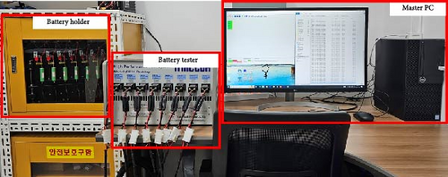
Figure 1 shows the performance experiment setup. The experiment uses a control device from Maccor Inc., [26] capable of supplying voltage/current, along with a PC for experimental control and a battery holder. There are eight LIBs used in the experiment, each with a nominal voltage of 3.7 V and a nominal capacity of 2.5 Ah. The detailed specifications of the equipment and LIBs are shown in Table 1.

Table 1. Specification of the Maccor’s equipment and LIB.

Maccor‘s equipment		INR 18,650 LIB
Items	Specification	Items	Specification
Channel	8	Cathode	NCA
Max voltage	20 V per channel	Nominal capacity	2500 mAh
Max current	5 A per channel	Charge	CC: 1.25 A/cut-off: 4.2 V CV: 4.2 V/cut-off:125 mAh
Control resolution	0.001	Max continuous discharge	20 A
Record resolution	1	Useful life	1500 mAh at 250 cycle

2.2.2. Performance Experimental Procedure

The performance experiments conducted by our research group consist of aging experiments simulating the operating environment of LIBs and reference experiments to assess the health state of the LIBs. The detailed experimental procedures performed are shown in Algorithm 1.

Algorithm 1: Battery performance experiment procedure.

• Q_init, Q_init                    ⊳Nominal/Aged capacity

• E                       ⊳Available threshold(%)

• V_max, I_max                  ⊳Maximum voltage/current

• t_dis                    ⊳Operating time for discharge

• whileQ_aged > Q_init × Edo

•   j = 0, I = 0.5C

•   whilej < 2do                         ⊳Start RP

•     Full charge                        ⊳CC-CV

•     Rest for 15 min

•     Full discharge at I

•     Rest for 15 min

•     j = j + 1

•   end while

•   Q_aged ← f(I, t_dis)               ⊳Coulomb Counting

•   k = 0, n = 0

•   whilek < 10do                       ⊳Start AP

•     Full charge                        ⊳CC-CV

•     Rest for 10 min

•     whilen < 20do

•       I = rand[0.5CtoC_max]

•       Load at I for 5 min

•       if V < V_mim then cut-off

•       end if

•       n = n + 1

•     end while

•     k = k + 1

•   end while

• end while

In Algorithm 1, the reference process (RP) aims to identify the maximum available capacity of aged LIBs as the experiment progresses. For clear capacity identification, the remaining capacity of the LIB must be considered. Therefore, in the RP, two full charge/discharge cycles are conducted: in 1-step, the remaining capacity of the LIB is initialized, and in 2-step, the maximum available capacity is derived. The capacity is derived based on the Coulomb counting method [27] and is expressed as follows:

$$ ()

where t is the time taken and I is the current. The aging process (AP) is designed to consider various operating environments of LIBs, with discharge performed based on randomly configured current profiles:

$$ ()

where n represents the number of discharges performed during one AP cycle. The number of discharges is derived from the nominal capacity and has the following relationship:

$$ ()

where Ah_fresh is the nominal capacity of the LIB, t_i and I_i are the discharge time and discharge current per step in the AP process. The detailed conditions of the performance experiments are shown in Table 2.

Table 2. Experimental condition in Lab.

Condition	Process
	Reference	Aging
Charge (CC-CV)	CC: 1.25 A charge, 4.2 V cut-off CV: 4.2 V charge, 125 mA cut-off
Discharge	1.25 A discharge 3.2 V cut-off	Rand (1.25 to 5 A) Max 5 min
Cycle	2	20

The charging method follows the CC-CV specified in the LIB specifications in Table 1. The random current profile is generated from Equation (2), and the maximum discharge current is set to 5 A, the maximum allowable current based on the equipment specifications in Table 3. The number of discharges is derived from Equation (3), and considering the reduction in available capacity and the range of discharge currents as the experiment progresses, it is set to 20 cycles.

Table 3. Possible battery failure situations [6].

Failure situations
Case	Factor	Impact
Misuse	Overcharge/discharge	Overheating acceleration internal damage
Shock	Crash
Cell balancing	Internal damage overcharge/discharge	Potential difference increase internal resistance
Thermal	Self-heating due to internal resistance ambient temperature	Explosion shutdown
Temporary loss of capacity	Power consumption	Power off increase internal resistance
Permanent loss of capacity	Repeated charge/discharge internal damage	Decrease useful capacity

2.2.3. Result and Analysis

Figure 2 shows the results of the RP experiment. Figure 2a shows the voltage/current plots recorded during two repeated full charge/discharge cycles, and Figure 2b shows the charge/discharge capacity. In 1-step, the charged capacity is less than the discharged capacity, indicating that residual capacity was present in the battery during charging. In 2-step, it can be observed that the charged and discharged capacities are the same, confirming that the battery’s capacity was correctly initialized in the preceding discharge. These results confirm that two continuous full charge/discharge cycles are an appropriate procedure for identifying the battery’s maximum charge capacity.

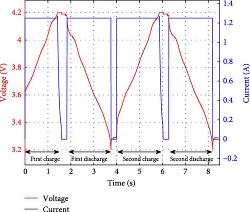
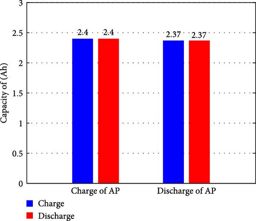
Figure 3 shows the results of the AP experiment. Figure 3a shows the voltage/current plots recorded during the charge/discharge cycles, and Figure 3b shows the charged capacity and accumulated discharged capacity. From Figure 3a, it can be seen that the experiment proceeds satisfying the set discharge time of 5 min in the first half of the experiment. However, in the second half, the set discharge time of 5 min is not met. From the results of Figure 3b, it can be inferred that the charged capacity was completely depleted, preventing further discharge.

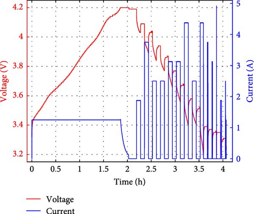
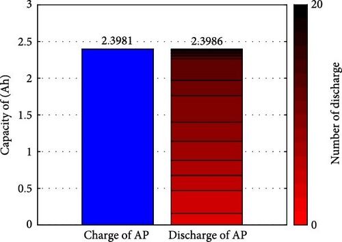
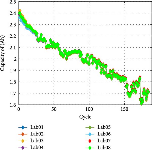
Figure 4 shows the results of the performance experiment. Figure 4a shows the capacity degradation histories for the eight LIBs used in the experiment, showing a decrease in maximum available capacity as the experiment progresses. Figure 4b compares the results of the first performed AP (top) and the last performed AP (bottom). It can be observed that the number of times the 5-min discharge condition was satisfied decreased from 8 to 6 due to the reduced available capacity, resulting in a decrease in AP duration.

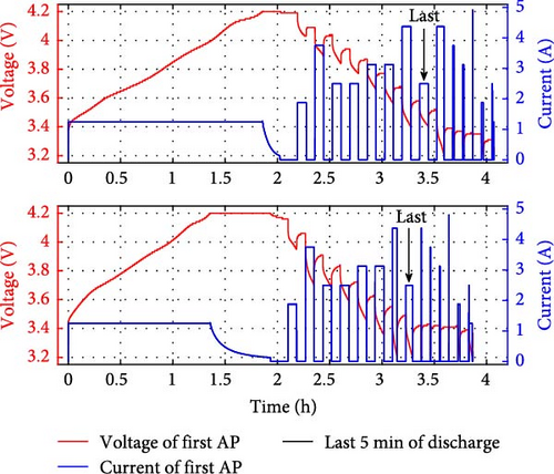
These experimental results indicate that even with the same discharge current, the voltage, remaining capacity, and other factors vary depending on the discharge timing and battery status.

2.3. Battery Data in NASA

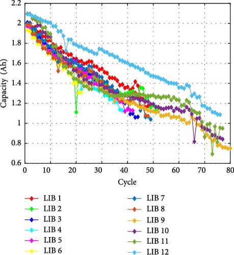
The additional data utilized in this study were sourced from the publicly available datasets provided by NASA Ames PCoE [28], consisting of time-series data (voltage, current) obtained from charge/discharge experiments. Twelve LIBs (cathode: NCO) were used in these experiments, each with a nominal voltage of 3.7 V and a nominal capacity of 2 Ah. The detailed experimental conditions are presented in Table 4.

Table 4. Experimental condition in NASA.

Condition	Process
	Reference	Aging
Charge (CC-CV)	CC: 2 A charge, 4.2 V cut-off CV: 4.2 V charge, 125 mA cut-off	Rand (0.5–4 A) Max 5 min 4.2 V cut-off (charge) 3.2 V cut-off (discharge)
Discharge	1 A discharge 3.2 V cut-off

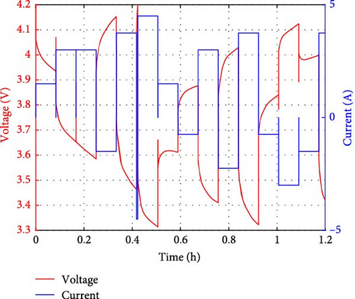
NASA’s AP is based on a profile composed of random currents within the range of [0.5 A, 4 A], where charging and discharging are performed for up to 5 min. In this process, the charging and discharging are not performed sequentially but randomly, so that two or more consecutive charging or discharging cycles can be performed. Figure 5 shows the experiment results of NASA. Figure 5a shows the recorded voltage/current during 15 cycles of the AP process, and Figure 5b shows the capacity degradation histories throughout the experiments.

3. LIB Diagnostic Dataset

In this section, we extract data for health state diagnosis from both laboratory experiments and publicly available datasets and construct input/output data for model training.

3.1. State of LIB

3.1.1. State-of-Health (SOH)

The SOH of LIB considered in this study is a percentage representing the degree of aging progress, which is used as an indicator to determine whether to use LIB, and is defined as follows based on permanent capacity loss:

$$ ()

Here, Ah_loss represents the permanent capacity loss due to aging, Ah_available represents the available capacity obtained from RP, and Ah_loss increases as aging progresses. Thus, SOH derived based on Ah_available can identify the degree of aging of the LIB.

3.1.2. End-of-Life (EOL)

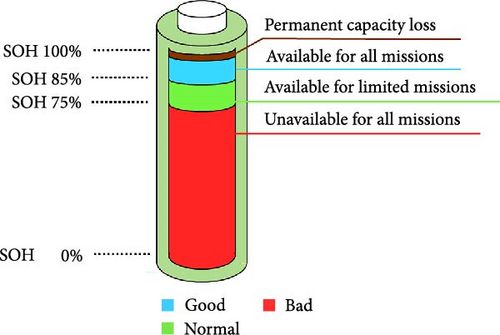
EOL signifies the recommended point to cease using the LIB. Beyond this point, the aging level is so high that performance and safety cannot be guaranteed. Therefore, EOL is defined based on the previously defined SOH and is set within the range of SOH 80% to 70%, depending on the operational conditions.

3.1.3. Level of State

In this study, we categorize the usability of LIBs into three levels, taking into account their discharge performance and operational environment in relation to EOL. Here, EOL is set 5% higher to account for uncertainties such as recovery effects.

• •

  Good: SOH of 85% or higher, indicating minimal impact from aging and suitability for use in all environments.

• •

  Normal: SOH of 75% to less than 85%, indicating that the effects of aging have occurred. Use is restricted in environments requiring SOH of 85% or higher but allowed in environments requiring SOH of 75% or higher.

• •

  Bad: SOH of less than 75%, indicating significant impact from aging. Performance and safety cannot be guaranteed, thus deemed unsuitable for use in all environments.

Figure 6 shows the LIB usability levels (good, normal, and bad) considering two different EOL thresholds.

3.2. Inspection Data of LIB

3.2.1. HI

The HI is a parameter used to analyze the health state of LIB. In this study, the time-series discharge data to be utilized records voltage and current information over time during battery usage, making it useful for tracking and analyzing real-time changes in battery status.

However, the length of time-series data is inconsistent depending on the recording time, and data loss may occur when performing additional tasks such as postprocessing. Therefore, to extract effective aging parameters from time-series discharge data, it is essential to capture and utilize singularities that occur with time changes.

3.2.2. Input Data

In general, LIBs emit a fixed current (rated current) depending on what they are powered from, so they have a constant current characteristic with little variation in current. On the other hand, the voltage of the LIB tends to decrease nonlinearly as the discharge progresses. This means that the shape of the discharge voltage curve can vary depending on the discharge time and discharge current. Thus, voltage-based aging parameters should be derived considering the discharge time, decrease tendency, etc. Therefore, in this study, summary statistical variables and distribution statistical variables are utilized to effectively capture the singularities of time-series voltage data.

• •

  Summary statistics: Summary statistical variables describe the variation in the data in a simple way, making it easy to analyze the key points and general trends in the data. In this study, six summary statistic variables were used: start, end, maximum, minimum, start/end voltage difference, and voltage difference between maximum and minimum.

• •

  Distribution statistics: Distribution statistics are variables that can represent the distribution of the data, making it easy to analyze the diversity of the data. In this study, four distribution statistics (mean, standard deviation, kurtosis, and skewness) were used. In particular, kurtosis and skewness are figures that indicate the shape of the data distribution, representing the degree of peakedness and asymmetry, and are expressed as follows:

  • -

    Kurtosis (Kur):

    $$ ()

  • -

    Skewness (Skew):

    $$ ()

Here, n represents the length of the data, x_i represents the value of the variable over time, and μ and σ represent the mean and standard deviation of the input data.

Therefore, the inspection data for analyzing the condition of LIBs consists of a total of 13 items as follows:

$$

3.2.3. Output Data

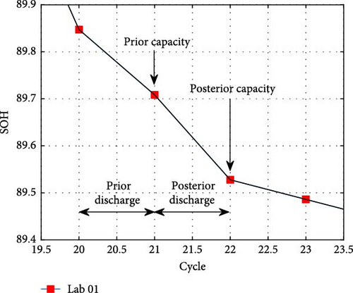
The LIB health state diagnosis system proposed in this study analyzes the input data defined above and outputs the SOH at the recorded time. In other words, this requires the SOH corresponding to the partial discharge data acquired from the AP. However, since it is not possible to obtain SOH based on partial discharge data, it is used by interpolating the SOH obtained in the previous RP and the SOH obtained in the next RP. Figure 7 shows the correspondence between the AP process and the RP process.

4. R-DNN–Based LIB Health Diagnosis System

This chapter describes the construction of a training model and evaluation metrics for LIB health diagnostics.

4.1. R-DNN–Based Classification Model

The DNN refers to a neural network with more than three hidden layers between the input and output layers. By passing through the hidden layers, the activation function allows nonlinear combinations among the input variables, enabling the modeling of complex nonlinear relationships. The DNN-based classifier for diagnosing LIB health state is designed to increase the number of neurons as the depth of the hidden layers increases, allowing the extraction of complex features. In this study, GELU [29] was used as the activation function, and its equation is as follows:

$$ ()

However, such deep and wide networks can lead to overfitting. To mitigate this, residual connections were applied to the DNN. Figure 8 shows the flow of residual connections.

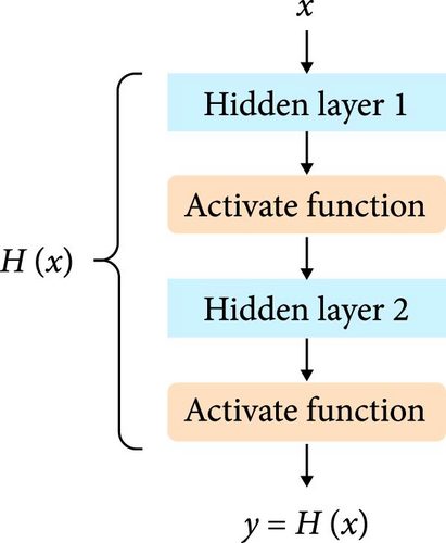
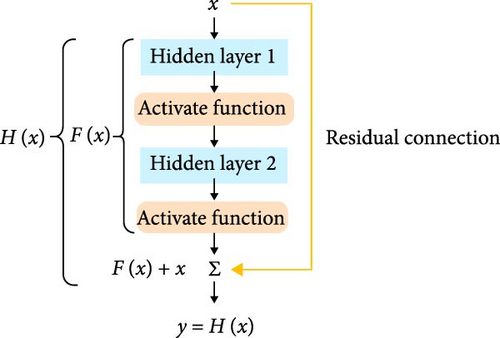
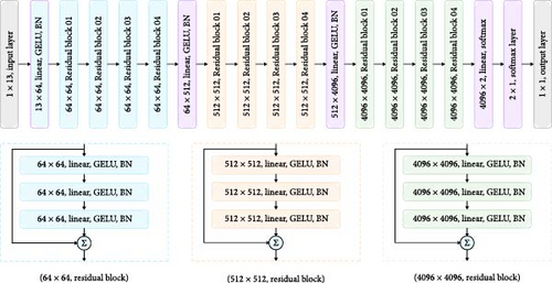
Residual connections prevent data loss during layer transitions by passing information from previous layers. This role allows the deep model, even with over 100 layers, to learn correctly without overfitting [30]. Additionally, batch normalization was applied to all hidden layers to improve training speed and stabilize the model. Figure 9 shows the structure of the constructed R-DNN.

4.2. LIB State Diagnosis System

During the training process, the classification model creates a hyperplane that can separate the data through parameter updates. This creation process cannot be directly controlled, which is both a characteristic and a limitation of deep learning, potentially leading to incorrect classification results. Therefore, it is crucial to guide the proper creation of the hyperplane.

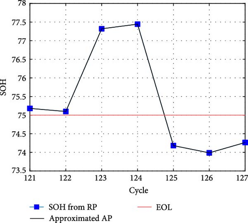
Figure 10 represents a part of the RP experiment, showing the point where the state changes from “normal” to “bad.” Due to the threshold, the AP discharge data performed after the 124th RP is classified as “bad,” but it can be observed that not all data are “bad.” This is due to the continuity of the data, indicating the limitations of labeling. It is important to minimize the uncertain data labeling results because it is a factor that adversely affects the learning model.

In this study, we propose a stepwise diagnostic approach using an R-DNN-based classifier. Figure 11 shows the conceptual diagram of the health diagnosis system.

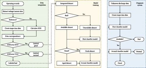
First, the primary classifier determines availability, outputting results as “bad” or “else.” If the result is “else,” the input data are passed to the secondary classifier. The secondary classifier then determines suitability, outputting “good” or “normal.” This approach reduces incorrect classifications at two boundary areas. Additionally, independently configured classifiers allow for efficient management and utilization through individual approaches.

4.3. Performance Evaluation Metric

The performance of the trained model is evaluated using a confusion matrix. The confusion matrix shown in Figure 12 is a table visualizing the classifier’s results, composed of a combination of prediction success (true or false) and prediction results (subscript). Since the classifier used in this study aims to diagnose the state of the LIB, the LIB health level is designated as the class.

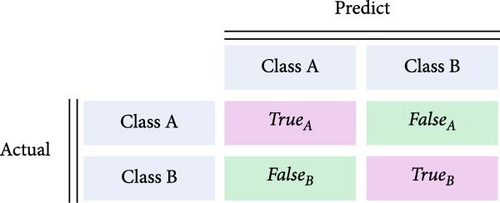
The evaluation metrics using the confusion matrix are recall and precision, defined as follows:

• •

  Recall (R_state):

  $$ ()
  Recall is defined as the ratio of predicted results corresponding to the input data for a specific class. Since it is derived based on the input data, the model’s classification success rate for a specific class can be evaluated.

• •

  Precision (P_state):

  $$ ()
  Precision is defined as the ratio of input data corresponding to the predicted results for a specific class. Unlike recall, it is calculated based on the prediction results, allowing for an evaluation of the model’s accuracy.

5. Train and Validation

This section trains and validates the LIB health state diagnostic model.

5.2. Training LIB State Diagnosis Model

5.2.1. Loss Function

In general, cross-entropy is used in classification models. However, cross-entropy considers only misclassification over the entire dataset, which can lead to biased results if the data are imbalanced among classes. To address this, the focal loss function, which considers class imbalance, was used in this study and is defined as follows [31]:

$$ ()

where n and C are the number of data and categories. L and P are the true value and the probability of the true value. α and γ are variables that adjust the value of the loss, assigning weights to the calculated error.

5.2.2. Hyperparameters

The training parameters used for the proposed model are listed in Table 6. The model is trained iteratively over a specified number of epochs, using randomly selected data in batches. Furthermore, if the model fails to improve for a specified number of patient iterations during training, early stopping is applied.

Table 6. Hyperparameters for R-DNN model train.

Batch size			Adam optimizer		Focal loss		Scheduler
Epoch	Train	Validation	Learning rate	Weight decay	α	γ	Iteration	Factor	Early stop
1000	512	256	1e-3	3e-4	0.25	2	30	0.05	30

5.2.3. Training and Validation

Figure 13 shows the learning process of the acquired models.

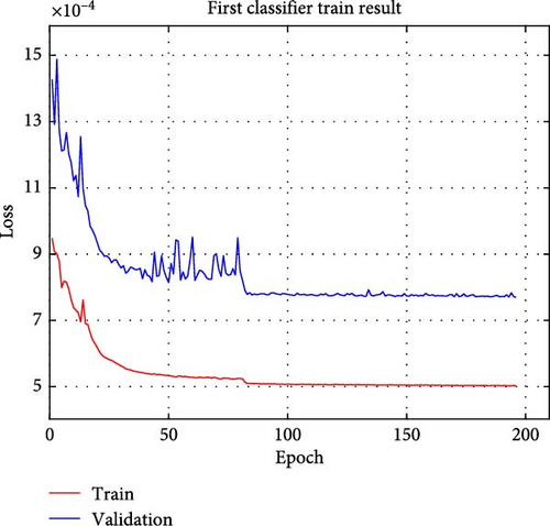
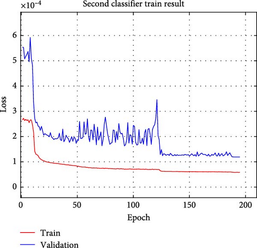
Both trained models stopped training without reaching the defined 1000 epochs, which is due to the fact that they did not improve their performance despite repeated training and were terminated prematurely. As a result, the final obtained model was generated 30 epochs before the end of the training epoch.

Table 7 presents the evaluation results for the training and validation of the primary and secondary classification models. The three evaluation metrics for both training and validation show errors within 3%, indicating similar performance. This indicates that no overfitting occurred and that the training was conducted properly. In particular, the recall, which indicates the diagnostic success rate, is approximately 90% or higher, indicating the model’s capability for satisfactory diagnosis.

Table 7. Learning performance of the trained model.

Train	First classifier		Second classifier
	Else (%)	Bad (%)	Good (%)	Normal (%)
Recall	91.25	94.08	91.00	89.11
Precision	96.39	86.10	89.91	90.27
F1-score	93.75	89.91	90.45	89.68
Validation	Else (%)	Bad (%)	Good (%)	Normal (%)
Recall	93.23	93.92	90.29	90.30
Precision	96.39	88.86	90.80	89.77
F1-score	94.78	91.32	90.54	90.30
			Else: good + normal

5.3. LIB State Diagnosis Model Test

5.3.1. Model Test and Analysis

In this section, we evaluate the validity of the learning model on data that were not encountered during training, that is, LIB08 data obtained from the laboratory and NASA Bat03 data, which were not utilized during training. Table 8 shows the evaluation results for model evaluation.

Table 8. Test performance of the trained model.

Test	First classifier		Second classifier
	Else (%)	Bad (%)	Good (%)	Normal (%)
Recall	95.62	89.70	92.74	91.98
Precision	95.86	89.15	91.13	93.45
F1-score	95.74	89.42	91.93	92.71
			Else: good + normal

Firstly, the test results for the primary classifier show approximately 90% recall and precision. This indicates high diagnostic performance in identifying “bad,” with a low likelihood of incorrect diagnoses. Second, the test results for the secondary classifier also demonstrate recall and precision above 90%. This indicates high performance in distinguishing between “good” and “normal” states. Considering that these results are obtained using data not involved in the training, it implies that the model can effectively assess the usability and suitability of LIBs using partial discharge data.

5.3.2. Comparative Analysis

In this study, we trained a comparison group model and analyzed its performance to verify the validity of the proposed model. We compared the performance difference between models using time-series data and models using statistical data. We further analyzed the performance of models with and without residual blocks. Figure 14 shows the evaluation results of the proposed model and the comparison group model, and additional neural networks were constructed to compare the diagnostic performance according to the neural network structure.

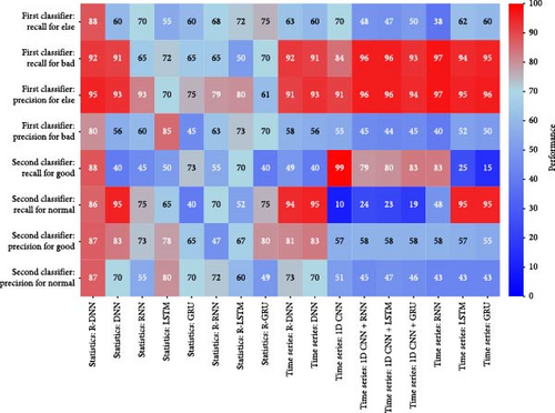
The models using time-series data showed unsatisfactory performance overall, with biased results. The RNN model with time-series data had a very low recall of 38% and a precision of 52% for “else.” The LSTM and GRU models also performed poorly with only 40% and 50% recall for the Else label, respectively. These results indicate that neural network models using time-series data do not sufficiently learn temporal patterns, leading to performance bias.

In contrast, the models using statistical data were more stable and performed well. The DNN model using statistical variables performed better than the DNN using time-series data, with 60% recall and 93% precision for “else.” This shows that statistical input data provide better information for training than time-series data, which contributes to reducing performance bias.

Also, models that applied residual block performed better than those that did not. The residual block was effective in mitigating the problem of gradient decay as the neural network deepens, thereby improving performance in deeper neural networks. In particular, the R-DNN model using statistical data outperformed DNN on all performance metrics, demonstrating the positive impact of the residual block on improving the performance of neural networks.

On the other hand, to analyze the performance according to the structure of the LIB health diagnosis system, we constructed and trained a unified (not divided into primary and secondary) health state diagnosis system. Table 9 presents the comparison results based on system architecture.

Table 9. Compare diagnostic results to system structure.

	Sequential classifier		Multiclass classifier
	Recall (%)	Precision (%)	Recall (%)	Precision (%)
Good	93	91	92	88
Normal	85	86	81	84
Bad	90	89	88	88

The model in a unified system configuration has three candidate states to diagnose. Therefore, each state has two potential misdiagnoses, affecting the recall and precision of each state. In contrast, the system proposed in this study performs a sequential diagnostic process to reduce misdiagnoses. This approach improves recall and precision performance, resulting in overall performance enhancement.

Through this comparative process, it is evident that the sequential diagnostic method of the proposed system is effective in assessing usability and suitability.

6. Conclusions

In this study, we propose the R-DNN–based diagnostic system for diagnosing the health state of LIBs. To train the model, we utilized laboratory data and NASA data and selected partial discharge data to consider various operational situations of the LIB. To effectively consider the length and degradation characteristics of time-series discharge data, statistical variables were used to generate diagnostic data, which served as the input to the system. Additionally, the health state of LIBs was defined in three levels based on maximum chargeable capacity and equipment’s required output, which were designated as the system’s output.

The diagnostic system comprises two R-DNN-based binary classification models, where the availability and suitability assessments are performed sequentially. The system’s validation and evaluation were conducted using recall and precision metrics derived from the confusion matrix, with both the primary and secondary classifiers showing recall and precision rates above 85%, indicating satisfactory diagnostic performance. Furthermore, the feasibility of the model structure configured in this study was confirmed by comparing performance changes across different neural networks and system structures.

In summary, through the comparison of training, validation, and test results, it was confirmed that despite numerical errors, the diagnostic data generation method using statistical variables was effective in diagnosing the defined three states. Additionally, the proposed diagnostic system can be extended to use various types of data as input, as it uses 13 statistically analyzed variables rather than time-series data as input.

Finally, since the current system considers only single-cell LIBs, it is expected that the diagnostic performance and utility of the system will improve with the appropriate enhancement of the model through the addition of multicell LIB data in the future.

Conflicts of Interest

The authors declare no conflicts of interest.

Funding

This research was supported by Unmanned Vehicles Core Technology Research and Development Program through the National Research Foundation of Korea (NRF), Unmanned Vehicle Advanced Research Center (UVARC) funded by the Ministry of Science and ICT, Republic of Korea (2020M3C1C1A01083162), and by the Technology Innovation Program (RS-2024-00508291, development of integrated package for optimal operation of 100 m class OSV) funded by the Ministry of Trade, Industry and Energy (MOTIE), Korea.