An Optimal Fast Frequency Control Method for Variable Speed Wind Turbines Based on Doubly Fed Induction Generators Through Simultaneous Control of Frequency and Maximum Torque
Abstract
The need to mitigate environmental pollution and conserve the environment has led to the rapid expansion of renewable energy sources (RESs) and wind farms (WFs) in power systems. Thus, the involvement of WFs in frequency control and raising the frequency nadir (FN) under transient conditions of the system will be highly significant and indispensable. This research presents a proposal to enhance the system frequency by utilizing WFs and restoring the speed of the wind turbine (WT) rotor using the doubly fed induction generator (DFIG) while avoiding frequency second dip (FSD). In this design, once the disturbance and decrease in the system frequency are identified, the new power reference is incorporated into the maximum power point tracking (MPPT) characteristic as a function of two parameters, the changes in system frequency and the speed of the WT rotor, taking into account the torque limit. During frequency support, the frequency change parameter increases, while the rotor speed parameter decreases. This results in a smaller decline rate of the reference power, so that the electrical power goes below the mechanical power with a smooth gradient, not a step-wise manner. As a result, the rotor speed is restored fast without FSD. Another benefit is that the MPPT characteristic qualities are maintained during the frequency support, as the new reference value is incorporated into the MPPT characteristic. The MATLAB simulation results of the test system demonstrate that the proposed design successfully enhances the system’s frequency without inducing a FSD. Additionally, it effectively and rapidly restores the rotor speed.
1. Introduction
According to the European Council agreement cited in [1], in October 2014, it was determined that at least 27% of the final energy consumption in 2030 should come from renewable energy sources (RESs) to decrease greenhouse gas emissions from traditional energy systems. As stated in the European Energy Roadmap [2], this proportion should rise to a minimum of two-thirds by 2050. However, the growing use of RES in power systems comes with a set of issues that have been consistently addressed in the past few decades [3, 4].
The primary challenge lies in the fundamental characteristics of these resources, namely, their unmanageability [5], uncertainty, and variability [6, 7]. Specifically, fluctuations in the mid-term (within minutes) and short-term (within seconds) have a detrimental impact on the system’s reliability and lead to a decline in the frequency quality of the system in both grid-connected modes [8, 9] and islanded mode [7, 10]. A further challenge arising from the growing adoption of renewable energies is the need for conventional power generation units, such as synchronous generators (SGs), to operate with greater flexibility and at reduced load levels, or even temporarily shut down. Eliminating a component from the system results in a decline in life expectancy and a rise in expenses. Additionally, it diminishes the backup capacity of SGs for regulating the primary and secondary control of the system frequency [11, 12].
The third challenge of RES, as seen in Figure 1, involves the reduction of the synchronous inertia of the system. RESs are often linked to power systems via electronic power converters. When there is a modification in the inertia value of the system, the inertial response (IR) of the system will correspondingly alter. The greater inertia of the system results in a reduced rate of change of frequency (ROCOF), and the frequency nadir (FN) is maintained at higher levels [12]. The phenomenon can be explained by the fact that in conventional power grids, when there is a disturbance in the generation or consumption of electricity, SGs automatically supply the necessary active power and inertia to the system by converting the stored kinetic energy (KE) in the rotating masses. This mode is referred to as IR, which has a stabilizing influence on the frequency of the grid, so aiding in restoring the frequency to an acceptable level. However, as renewable energies, particularly wind power, become more prevalent in power systems through electronic power converters, the turbine’s rotational speed becomes independent of the grid frequency. This leads to a decrease in the system’s overall inertia, resulting in a reduced IR. Nevertheless, both the rotor of a variable speed wind turbine (VSWT) and a generator directly connected to the grid possess KE that can be used to enhance the grid frequency [15, 16].

With the growing integration of wind power into power systems, ensuring frequency stability within the desired range has become a crucial study topic [17, 18]. Wind energy conversion systems (WECSs) are necessary in northwest China’s power grid to maintain frequency stability during disturbances [19, 20]. However, the challenge with VSWT is that operate in maximum power point tracking (MPPT) control mode when the wind speed (WS) is below the rated value. In this mode, the turbines continue to operate independently and do not release the power generated by the KE of the rotating mass. As a result, they do not contribute to improving the grid frequency. Thus, to address these difficulties, the key technical prerequisites, including active and reactive power regulation and wind farm (WF) response during grid disruptions, have been identified [21, 22]. Various techniques have been proposed to involvement of wind turbine (WT) generators in the short-term assistance of grid frequency [23, 24].
When the WS is below the nominal speed, there are two categories of research and strategies. VSWTs in the first group operate without any load to maintain a reserve of active power. This allows them to be utilized for temporary frequency support (TFS) of the system [25, 26]. While these methods effectively conserve electricity and offer appropriate frequency support as required, operating WTs without a load under normal conditions might result in financial losses for WF owners, which is undesirable.
Within the second category, WTs operate at WSs below the rated value, allowing them to efficiently harness the maximum power from the wind through MPPT control mode, resulting in no loss of income. WFs are often inefficient under normal operating conditions. However, in a disturbance, they can temporarily sustain the grid by releasing the stored KE from their rotating masses. However, the level of support that may be offered is inferior to that of the first group. Additionally, when it comes to frequency support, they cease to operate in the MPPT control mode, which presents some challenges. During frequency support, the power reference value exits the MPPT mode, and a new power additional (∆P) is considered the reference power. This new value indicates the amount of KE that can be released. Consequently, the speed of the rotor will decrease in response to the greater power. Once the grid frequency support finishes, the rotor speed should be promptly increased to return to the original operating position in the MPPT prior to the disturbance [27, 28]. Hence, the challenge is to ensure that the reference value of the newly added power is not excessively high, as this would result in a significant decrease in rotor speed and a prolonged restoration time. Because if the rotor speed is restored in a shorter time, a second frequency drop will also occur. If the incremental power reference value is minimal, the grid frequency will receive less support and cannot sustain a higher frequency level [29]. To address the aforementioned issues and provide temporary support for the system’s frequency, the authors have put up several recommendations involving the use of WTs. In [30], the author suggests a reliable control system for WFs employing adaptive gains for doubly fed induction generator (DFIG) and then proceeds to compare his scheme with fixed gain techniques for small and big WFs. Furthermore, they demonstrate the efficacy of his design in enhancing FN, although it fails to address the procedure for reinstating the rotor speed. The WF’s frequency adjustment is achieved by using time-varying inertia and loss controllers. In [31], the WF frequency is regulated via time-variant inertia and droop controls, and the gains are determined by considering the response time of the target frequency. The designs presented in [32, 33] primarily address the gain design for controlling additional frequency change rate loops to ensure the stable operation of WTs. However, these designs do not mention the rotor speed restoration strategy or FN under high and medium WS. Additionally, the rotor speed restoration in these designs occurs over a significantly more extended period.
Another set of publications has concentrated on the restoration of rotor speed, aiming for a rapid restoration within 30–70 s. However, their main challenge is to prevent a subsequent decrease in system frequency throughout the restoration process. The frequency second dip (FSD) is detected by analyzing the rate of change of active power and the rate of change of rotor speed, as shown in [29]. To prevent a sudden decrease in active power after the end of the frequency support, the square method is employed. The specific parameters of this method are calculated using the MPPT method. A time-varying drop characteristic is proposed in [34] to facilitate the seamless electric power exchange between WTs and the grid. Additionally, this approach aims to mitigate the FSD that occurs during the restoration of rotor speed. To do this, WF turbines are categorized, and their speeds are restored accordingly. The study examined speed restoration in single-stage and multistage modes according to the drop characteristic, and it showed that speed restoration in categorized turbines with determined periods results in FSD. To provide TFS, a predetermined constant power reference is implemented and must be changed based on the wind power penetration level (WPPL) [35]. To restore the rotor speed and return to the operating point of the MPPT curve in this design, a time interval is applied once the electrical power is equal to the mechanical power. The issue with this design is that choosing a short time interval for rotor speed restoration results in a fast restoration but can lead to a significant and severe decrease in frequency. On the other hand, selecting an extended time guarantees a very modest FSD, but the rotor speed restoration will be significantly slow. Kang et al. [36] have suggested a design for WT that utilizes a DFIG and incorporates a torque limit. This design allows for the efficient release of a significant quantity of KE, enhancing the frequency. Subsequently, the power diminishes linearly when the rotor speed is reduced. In this design, the rotor speed is restored after the frequency support period by introducing a new power reference in the form of a minor step of 0.03 p.u. This new power reference is set at a value lower than the mechanical power, resulting in a small FSD. Furthermore, this newly established reference is upheld until it reaches the pinnacle of the MPPT curve.
Based on the aforementioned papers and the preceding analysis, this article has introduced a frequency support system that combines the benefits of both groups of articles described before. The proposed design allows for the release of a significant amount of KE and contributes to the system frequency, thanks to the high limit of the rotor torque. This ensures stable performance of the WT in varying WS, different WPPL, and rapid restoration of the rotor speed to the operating points of the MPPT curve while avoiding any FSD. By incorporating an adjustable gain and multiplication into the control loop, it becomes possible to accommodate various WS and WPPL. The process of determining and quantifying the potential quantity of KE that can be released is dependent on two factors, the frequency changes of the system and the speed of the rotor, which are determined by the torque limit. During frequency support, the frequency change parameter increases, while the rotor speed parameter decreases. This results in a smaller decline rate of the reference power, allowing the electrical power to go below the mechanical power in a smoothly and gradually, resulting in fast restoration of the rotor speed without any FSDs.
During the system frequency support, the new power reference is included in the existing MPPT characteristic. Thus, while temporarily sustaining the system’s frequency, measuring the MPPT retains its benefits and aids in stabilizing and enhancing the system during WS fluctuations. Ultimately, after the power additional reaches zero, only the MPPT characteristic remains in the control circuit. Consequently, WT can quickly provide frequency support and return to their normal operating state without triggering an FSD. Typically, all methods used to manage the inertia and frequency of WTs are categorized within the 10-s interval for IR and the primary control (PC) interval, as shown in Figure 1, so that enough time is provided to increase the governor percentage, adjust other SGs’ fuel, and increase active power. Consequently, returning the frequency to its original value before the event relies on the grid’s SGs and the secondary and tertiary control loops. However, this article does not cover this topic. The subsequent sections of the essay are organized as follows: Section 2 focuses on WT modeling and control of DFIG. Section 3 focuses on the suggested approach for temporarily supporting system frequency by WFs using induction generators. Section 4 analyzes the effectiveness of the proposed plan, whereas Section 5 provides a discussion and conclusion regarding the proposed strategy.
2. Modeling WT and Controlling DFIG
Figure 2 depicts the arrangement of a DFIG and its controllers. These controllers consist of two electrical controllers, namely, the grid-side converter (GSC) and the rotor-side converter (RSC), as well as a mechanical controller that adjusts the pitch angle of the turbine blade. The RSC controller is responsible for regulating the reactive power injected into the power system and adjusting the rotor speed of the DFIG to optimize power absorption. It also ensures that the stator’s output voltage and frequency remain constant. On the other hand, the GSC controller is in charge of controlling the DC link voltage [37]. The main variables of Figure 2 are defined in Table 1.

| Definition | Variables |
|---|---|
| Measured current on the grid side and rotor side | ir, ig |
| Reference currents on the grid side and rotor side in dq coordinate | ird ∗, irq ∗, igd ∗, igq ∗ |
| Blade pitch angle of the turbine | β |
| Measured voltage on the stator and rotor sides | Vs, Vg |
| DC link voltage reference and measured value | Vdc, Vdc ∗ |
| Reactive power reference | Q ∗ |
CPmax refers to the maximum possible value of CP for β = 0, established as 0.5. The optimal value of λ, referred to as λopt, is 9.9495. kg value is constant and has been assigned a fixed value of 0.512. An abrupt and disproportionate surge in power generation might result in mechanical strain on a WT. To avoid this, the power limit and torque restriction are established at 1.1 and 1.07 p.u., respectively [36].
3. The Proposed Scheme for Temporary System Frequency Support Using WF Based on DFIG
All frequency support studies pertaining to WFs are classified into two primary categories: (1) hidden inertia emulation and (2) fast power reserve.
The inertia value is computed and utilized as a power reference for the WF in the first category, based on the frequency change rate. The initial category effectively replicates the IR of conventional power plants equipped with SGs and applies this to WFs. The benefit of the first category is a more gradual recovery of rotor speed; nevertheless, it results in a reduced release of KE, and the duration required to restore rotor speed and revert to the prior operational point is significantly prolonged, occurring within the frequency secondary control range (Figure 1). The second category is short-term continuous power, referred to as fast power reserve. Fast power reserve can be achieved by regulating rotor speed, which optimally releases KE based on the WF’s capacity and rotor speed, thereby aiding system frequency [1, 22]. Consequently, the generated reference is more pragmatic and functional, thereby releasing the maximum KE. However, the problem of the second category is to return to the starting operating point without inducing an FSD.
The proposed design has been evaluated against the design that maximizes KE, and despite the subsequent challenges, the frequency enhancement in the proposed design has been demonstrated. Three primary issues complicate the balance between maximizing power output and achieving a gradual recovery of rotor speed, hence determining the optimal operating point and its impact on frequency levels.
The primary problem is that KE is often related to WS; so, with lower WS, the energy stored in the rotating mass is diminished. The second challenge is that if the KE of the WT is released immediately, it allows minimal time for other SGs in the network to respond.
Consequently, due to the leniency of the fuel supply systems and the governors of the SGs, SGs cannot compensate for the active power in a brief duration of energy. At the same time, WTs require energy to revert to their original operational state, which must be sourced from the SGs themselves (see yellow section in Figure 3). Consequently, the deficiency of network power will escalate, resulting in an elevation of the FN. Upon reverting to the normal operational state of the WT, an FSD will occur, and the frequency profile will be as follows [29, 34].

The third challenge pertains to the MPPT control technique, and since the proposed design is evaluated against the design that optimally releases KE, it is elucidated as follows.
Scheme 1 establishes a new power reference value in the ωr range for TFS. Upon detecting an event, as depicted in Figures 4 and 5, the power output of the turbine increases from P0, which represents the MPPT curve, to PTlim (ω0), which means the power output resulting from the maximum torque at ω0. This design optimizes the release of maximum KE by utilizing maximum torque, resulting in a significant improvement in the FN. Subsequently, the turbine power output falls from point B to point C by Equation (9) and ωr. As the speed of the rotor decreases, the electric power is directed toward point C, which is equivalent to the mechanical power Pm:


The term dPTFS/dt represents the gradient of segment BC in Figure 5, while dωr/dt is directly proportional to the length of segment AB in Figure 5. Figures 5 and 6 demonstrate that decreasing the initial velocity causes point B to shift toward the left along the PTlim power limit line. However, the maximum power value remains unchanged at the minimal rotor speed. Consequently, dPTFS/dωr rises. Furthermore, the value of dωr/dt at point B is greater for small initial velocity compared to large initial velocity. This means that the rate of change of velocity is higher when the initial velocity ω0 goes toward the left side of the diagram. Hence, dPTFS/dt, at point B, which represents the highest deceleration rate during the deceleration period, is significantly greater for lower initial speeds compared to higher initial speeds. Consequently, a large dPTFS/dt over time persists for an extended duration. Consequently, additional SGs in the power system are required to supply more power to the grid for an extended duration to offset the decreased output power of a DFIG. As a result, the frequency is further reduced in this particular WF control method, leading to a delayed yet notable decline in the power system’s frequency. This tendency grows more pronounced with increased penetration of WFs. To prevent this, the proposed plan suggests using the reference power (PTFS) modified by the frequency deviation factor as stated in Equation (11). Upon event detection, a new ∆P value is promptly generated in the power reference. This value is derived from the combination of the rotor speed and the frequency difference ∆f. The value of ∆f is also compounded by an adaptive gain that considers the rotor speed and the extent of WPPL variations. This work results in a proportional increase in the generated power relative to the initial speed of the rotor, depending on the varying levels of WPPL.

The variable fnom represents the nominal frequency, while fsys represents the measurement frequency of the system. Thus, based on the MPPT in Figure 5, the increment in power reference will be smaller for speeds near the minimum, thus ensuring the prevention of FSD. However, unlike scheme 1, the restoration of rotor speed does not result in an immediate fall in output power. Instead, it occurs gradually and with a moderate decline. Any decrease in the output over 0.03 p.u. results in an immediate reduction in the system frequency, leading to a detrimental impact on frequency stabilization. The speed of the rotor in a WT indicates the amount of energy that can be harnessed. When the rotor speed decreases during the system frequency support, the new power reference, which considers the rotor speed, gradually decreases as well. The electrical power diminishes the output of the WT and compels it to track the mechanical power until the electrical power output of the WT matches the input mechanical power. Thus, at this specific operational state, depicted in Figure 7, the WT’s output power will be reduced compared to the power achieved with the MPPT control. In the context mentioned, frequency support decreases the power reference from point A to point C by reducing the rotor’s speed. This results in an automatic reduction of the electrical power generated by the WT along the DB curve, eventually stabilizing at point B. Point B is slightly lower than point A, representing the MPPT control.

Figure 7 illustrates the method of frequency support in the proposed strategy. The distance between BC operating points is determined by the combined impact of adaptive gain and frequency deviation. Additionally, utilizing frequency as a feedback input helps streamline the design of frequency support and enables automatic adaptation to various frequency events and system conditions. Furthermore, the utilization of rotor speed parameters enables the WT to autonomously and seamlessly transition between the operational points of the MPPT curve and the frequency support operation. On the other hand, the benefits of MPPT control are also maintained, which can adjust to changes in WS while controlling frequency. It remains within the MPPT curve even when providing temporary support to the system frequency. Additionally, it only requires the collection of one additional power reference. Over time, as the frequency deviation gradually reduces to zero, it results in a gradual decrease in the power reference. Consequently, it progressively and seamlessly reduces the output electrical power to a level below the input mechanical power of the WT, leading to the rotor speed beginning to restore its original value. As the speed of the rotor increases, the power also increases. However, when the nominal frequency increases, the value of ∆f eventually becomes zero. As ∆f becomes zero, the first term of the PTFS relation is eliminated, leaving only the kgωr3 term associated with the MPPT curve. This signifies the end of frequency support and results in the reference power having no additional value. Currently, the WT is operating in a mode where it tracks the maximum power point and the pre-event point. The proposed design not only enhances FN but also ensures the smooth and rapid restoration of the rotor speed without inducing FSD across various WSs and varying levels of penetration, whether high, medium, or low. Hence, the proposed controller is as given in Figure 8.

3.1. Adaptive Gain Performance

All parameters constituting the power reference and adaptive gain in this study, except the frequency change parameter (∆f), are contingent upon the WF and WT. Consequently, modifications and adjustments to these parameters are implemented directly, with only the time delay factors potentially influenced by electronic equipment and the specifications and capacity of the processor. Conversely, the determinants of the frequency change rate (∆f) and alterations in ROCOF and system inertia are the WPPL within the power system, as illustrated in Figure 10 [22]. Consequently, the alterations (∆f) will rely on the WFs, as well as the system’s inertia characteristics, owing to the use of the WPPL parameter in the adaptive gain. The reference value in the proposed plan is thus more realistic and tailored to the WFs capability.

As the amount of WPPL into the system increases, the coefficient n lowers; otherwise, there is a risk of a delayed FN event. The reason is that WTs are employed to rapidly offset the low output of SGs and uphold the frequency during the initial moments of a frequency event. Consequently, at a higher WPPL, the overall quantity of WTs will increase, resulting in a faster output and a reduced energy demand from each WT. Consequently, when the amount of WPPL in the system grows, the ∆P value will drop, along with the n value, which is influenced by the level of wind penetration. Conversely, the rotor speed factor ωr, depicted in Figure 11, indicates that at higher WSs, the proportion of power generated by the WT relative to the overall power generated by the system is greater. This leads to an increased ROCOF and larger FN for the same frequency event. Consequently, when WS increases, a greater amount of power additional and KE is released and enhanced the FN. When the WS decreases to the average level, the amount of KE stored in the rotor also decreases. As a result, there would be a smaller rise in the additional power output that will not lead to a significant decrease in the rotor speed. This work aids in mitigating the excessive decrease in rotor speed, even in the occurrence of consecutive frequency disturbances. Furthermore, it should be noted that any fluctuations in WS throughout the frequency support period will be promptly and automatically adjusted, ensuring the WT’s stability throughout the frequency support procedure. Figures 9 and 11 display the varying values of WPPL and the value of n, together with the impact of changing WSs and n on the additional power value ∆P.

Consequently, this strategy incorporates the new power reference into the MPPT characteristic as a function of two parameters, system frequency variations and WT rotor speed, based on torque limitations without delay.
Consequently, the substantial and intricate disturbance results in a frequency drop, necessitating compensation by an increase in active power. All frequency support systems utilizing WFs aim to inject the active power deficit from the WF into the grid, akin to SGs, hence enhancing the FN during the initial seconds to enable other SGs in the system to compensate for the lost active power. Thus, based on the response latency and the governor’s leniency in SGs, the involvement of WFs in frequency management affords SGs the necessary time to augment power output.
The augmentation of active power by WFs is contingent upon the facility’s capacity, specifically the WPPL and wind velocity. The rise in WPPL rate diminishes inertia, elevates FN, and alters ROCOF variations. Consequently, the significant issue posed by these approaches is the WPPL and the magnitude of WS. Consequently, significant and intricate disturbances (such as unit or line outages or the abrupt entry and exit of the synchronous motor) are not regarded as challenges in this context, as the WF will only discharge KE up to its capacity, determined by penetration levels and wind velocity, the extent of the disruption caused within the system [42, 43].
3.2. Changes of the Reference Power Relative to Frequency and Torque Parameter Changes
Figure 12 illustrates that the additional power amount (∆P) is influenced by two parameters, K2 and K1. The application of K2 considers the variations in both turbine speed and torque limit. K1 represents the frequency of the system. Hence, taking into account both these characteristics simultaneously enables the incorporation of both the power system’s conditions and the WT’s conditions in establishing the reference power value.

Branch K2 or PTFS provides us with the WT’s reference power or active output power based on the torque limit of the turbine, as depicted in Figure 13.

The K1 branch has a multiplying effect, resulting in the extraction of maximum KE from the WT. This also leads to the reference power remaining at its maximum value for an extended duration. Consequently, the power reduction curve is shifted to the right as much as possible. This ensures that the frequency returns to the permissible range. When the ∆f branch becomes zero, the electrical power goes below the mechanical power with a smooth gradient. Simultaneously, ∆P reaches zero, and the system’s control solely relies on the MPPT curve. Consequently, there will be no requirement to gradually decrease the electrical power compared to the PTFS design, and the speed of the rotor will be restored without resulting in an FSD. The reference power, considering the impact of branch K1, is illustrated in Figure 14.

To gain a deeper understanding of the impact of K1 on the reference power and the TFS at a WS of 11 m/s, we examined various percentage values for the branch ∆f or K1. The effectiveness of these values is presented in Table 2.
| K1 (%) | ∆P (p.u) | Pref-max (p.u) | Wind power (MW) | freqnadir | Simulation |
|---|---|---|---|---|---|
| K1 = 10% | 0.0628 | 0.7856 | 109.6 | 59.444 | 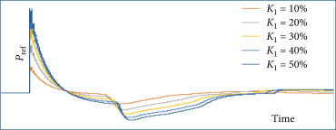 |
| K1 = 20% | 0.114 | 0.8368 | 116.8 | 59.6417 | |
| K1 = 30% | 0.1537 | 0.8765 | 122 | 59.7569 | |
| K1 = 40% | 0.1819 | 0.9047 | 126 | 59.8175 | |
| K1 = 50% | 0.1986 | 0.9214 | 129 | 59.852 | |
| K1 = 60% | 0.2038 | 0.9266 | 129 | 59.881 | 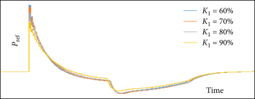 |
| K1 = 70% | 0.1976 | 0.9204 | 128.7 | 59.913 | |
| K1 = 80% | 0.1798 | 0.9026 | 126.2 | 59.9395 | |
| K1 = 90% | 0.1506 | 0.8734 | 122 | 59.9253 | |
Based on the findings presented in Table 2, it is evident that the reference power should be adjusted appropriately, and a trade-off needs to be made between the maximum power released and the gradual decline to restore the WT speed. Increasing the maximum power does not guarantee the stabilization of the FN at high levels. It may result in an FSD in the frequency spectrum. In the table, we have decreased the PTFS effect in proportion to the increase of ∆f to prevent the rise in released power, which could lead to significant variations and instability in the speed and output power of the WT. Figures 15–17 imply a negative rise in the output power during system frequency support. Reference values are selected as Pref1 < Pref2 < Pref3. Increasing the reference power will result in power fluctuations at the onset of frequency support.


Figures 15–17 illustrate that selecting an excessively large Pref and a significant reduction in rotor speed ωr should be avoided. Otherwise, the DFIG will function erratically. If Pref is configured to the highest power margin, a significant ωr decline will manifest more prominently for a minimal ω0, where the available KE for release is limited, due to its greater power margin. Moreover, selecting a larger Pref, particularly at moderate and low velocities, results in an extended duration of dPTFS/dt, which, coupled with the turbine’s instability, leads to a FSD. Consequently, to prevent excessive reduction of the rotor speed and to modify the power margin, is multiplied by the adaptive gain. In the adaptive gain, increases evenly concerning ω0, and contingent upon n, and is insignificant for very low ω0. This maximizes the value of Pref without excessive increase. Consequently, the turbine’s stability and its power output are assured.
4. Performance of the Proposed Scheme
4.1. Test System
A test system, depicted in Figure 18, has been utilized to assess the performance and validate the proposed design. The suggested design’s test system has been simulated using MATLAB software. The test system comprises a WF and six SG, with a static load of 73 and 220 MW, as well as motor loads defined by a 330 MW asynchronous motor. SGs 1 and 2 each have a capacity of 150 MV, SGs 3 and 4 each have a capacity of 200 MV, and SGs 5 and 6 each have a capacity of 100 MV. The time constant of inertia and characteristics of SGs are established according to the specifications provided in [36]. The additional parameters necessary for simulating WT and DFIG are provided in Table 3.

| Wind turbine/DFIG | Values |
|---|---|
| Nominal power (Pn) | 1.5 (MVA) |
| Nominal stator voltage | 0.575 (KV) |
| Nominal frequency | 60 (Hz) |
| Stator resistance | 0.023 (p.u) |
| Rotor resistance | 0.016 (p.u) |
| Stator leakage reactance | 0.18 (p.u) |
| Rotor leakage reactance | 0.16 (p.u) |
| Magnetizing reactance | 2.9 (p.u) |
| Turbine inertia constant | 4.32 (S) |
| DFIG inertia constant | 0.683 (s) |
| Pitch time constant | 0.01 (s) |
| Operating speed range | 0.70–1.20 (p.u) |
4.2. Different Simulation States
This section investigates the performance of the proposed scheme under different penetration and WS scenarios, comprising four other states:
State 1. WPPL: 20%; WS: 12 m/s
State 2. WPPL: 20%; WS: 11 m/s
State 3. WPPL: 50%; WS: 12 m/s
State 4. WPPL: 50%; WS: 11 m/s
The test system depicted in Figure 18 simulates the aforementioned scenarios. In the first and second states, the WF’s performance is analyzed and evaluated by monitoring the disconnection of SG number 4 within a 40-s time frame. As for the third state, one of the four 50–100 MW generators is removed from the circuit, and the WF’s performance is evaluated by analyzing the simulation results.
State 1. The WF has a wind penetration rate of 20% and a WS of 12 m/s. Figures 19–21 display the generation power of the WF, the rotor speed, and the frequency of the system, respectively. The proposed design has a 3.28% lower energy release than scheme 1. Additionally, the ∆P of the proposed design is 0.2954 p.u., which is much lower than the ∆P of scheme 1, which is 0.3944 p.u. The inclusion of FN in the suggested scheme exhibits improved conditions and has consistently maintained a higher frequency compared to scheme 1, as shown in Figure 21. The FN level is precisely 59.82 Hz, which represents an enhancement of 0.01 Hz compared to scheme 1. The explanation is attributed to the impact of the ∆f coefficient, which results in a reduced decrease in the rate of wind power generation compared to scheme 1. The extended duration allows the SGs to better accommodate the power additional requirement. Figure 20 demonstrates that the rotor speed in the suggested design has experienced a smaller decline than the original design. In scheme 1, the speed of the rotor has been decreased to 0.866 p.u. However, in the proposed design, the minimum rotor speed has been adjusted to a smaller value of 0.864 p.u. Additionally, the restoration of the rotor speed has commenced within a time frame of 69 s. Conversely, the rotor speed restoration is done automatically, gradually, and without interruption, taking ~5 s to reduce the electric power and restore the rotor speed. This effort not only reduces the mechanical stress on the rotor but also prevents FSD. Figure 19 shows that the proposed scheme allows for the gradual release of KE from the WT over time while ensuring the frequency sustained. Additionally, during the rotor speed restoration stage, the MPPT effect is maintained, and any variations in WS directly affect the output power of the WT. The WT consistently operates in MPPT mode, unlike scheme 1, which temporarily departs MPPT mode during the frequency support procedure.


State 2. The second scenario shows a reduction in WS, while the WPPL remains unchanged. In this scenario, the MPPT characteristic becomes more prominent. When the WS is higher and the WT operates at its rated speed, the power that can be harnessed from the WT remains constant and at its highest value. However, with WSs lower than the rated speed, specifically, the WT operates based on the MPPT curve. Thus, at the 40th second, when there is a disruption in generation and frequency support, the proposed plan is 1 MW lower than scheme 1. The corresponding ∆P value for the proposed plan is 0.1261 p.u., which is lower than 0.1337 p.u. of scheme 1. FN has fallen to 59.81 Hz in both cases. The simulation results of state 2 are depicted in Figures 22–24. The power reduction required to restore the rotor speed is 5 MW, and this reduction occurs over 4 s (from second 63 to second 67). The power lowers gradually during this time and then quickly begins to climb. This is due to the decrease in the ∆f impact and the increase in the ωr effect in PTFS. When the electrical power decreases by 5 MW, it becomes smaller than the mechanical power. As a result, ωr starts to increase. With the increase in speed, the electrical power also increases. This causes ∆f to become smaller until it reaches zero. Consequently, PTFS also becomes zero. Finally, just the impact of MPPT will persist. Hence, without switching, the frequency will be sustained using MPPT, which is a benefit of the proposed plan compared to all other conventional plans and scheme 1.


Figure 23 clearly illustrates that the proposed design reduces the rotor speed to 0.9248 p.u. at the 63th second and quickly returns to its original value. In scheme 1, the minimum rotor speed has decreased 0.9185 p.u. at the 58th second and takes longer to return to initial value. Therefore, the proposed design exhibits superior performance.
In state 3, the wind penetration has increased. According to the n diagram, increased wind penetration reduces n, resulting in lower ∆P. According to the proposed design, the ∆P will be lower compared to the first and second states. For the proposed design, the value of ∆P is 0.094 p.u., which is considerably lower than the value of 0.1332 p.u. for scheme 1. The simulation results of the third state are represented in Figures 25–27. At the 50th second, a portion of the generation is disconnected from the system. As a result, the proposed plan for frequency support, as indicated by ∆P, releases 0.05% of the KE, which is 13 MW less than scheme 1. Figure 27 illustrates that FN is identical at 59.72 Hz in the proposed design and scheme 1. Furthermore, Figure 25 illustrates that the electric power gradually decreases to restore the rotor speed. It is worth noting that the quantity of lowered electric power is comparatively lower than that of scheme 1, amounting to 5.5 MW within 4 s, which has a lower impact on SGs. However, in scheme 1, the reduction in electric power occurs in a stepwise manner and amounts to 9.6 MW. The power of 9.6 MW represents a twofold increase in the load on the SGs, which are responsible for compensating for the lost generation during frequency support. Figure 26 illustrates that the rotor speed in the proposed design reaches its lowest value of 0.945 p.u. after 74.6 s, decreasing from an initial value of 0.9872 p.u. In comparison, the rotor speed in scheme 1 reduces to its minimum of 0.92 p.u. in 68 s, resulting in a shorter restoration period than scheme 1.


State 4. Figures 9 and 11 indicate a relationship between the degree of wind force penetration and WS that has been previously described. When the wind penetration rises, the ∆P value will decrease. Similarly, when the WS drops, the ∆P value will also fall. The simulation results of the fourth state are represented by Figures 28–30. The WPPL has stayed consistent, and WS has decreased in contrast to the third state. Consequently, the value of ∆P will be less than that of the previous case. When a portion of the generation exits the circuit at the 50th second, the TFS plan is promptly initiated based on the ROCOF. The proposed design has a ∆P value of 0.090 p.u., which is lower than 0.111 p.u. of scheme 1. Figures 28 and 30 demonstrate that the power generated in the suggested design is 1.4% lower compared to scheme 1. This decrease in power has resulted in an increase of 0.02 Hz in the FN. Thus, it demonstrates the enhanced efficacy of the proposed approach in comparison to scheme 1.


Figure 29 shows that the minimum speed of the rotor in the proposed design has lowered from 1 to 0.96 p.u. in 76 s. In scheme 1, the minimum speed of the rotor has decreased to 0.9471 p.u. in 63 s. Thus, the proposed design exhibits a shorter rotor speed restoration time than scheme 1.
To enhance the precision and accuracy of the comparison, the simulation results for several states of the proposed design are presented in Table 4. Table 5 presents a comparison of several states for enhancing FN in the proposed design with other designs, which demonstrates the frequency enhancement achieved in the suggested design.
| WPPL (%) | Wind speed (m/s) | Number of wind turbines | Wind power (MW) | Max. wind power (MW) | Amount of increased power (p.u) | Improved nadir (Hz) |
|---|---|---|---|---|---|---|
| 20 | 12 | 79 | 98 | 118 | 0.2954 | 0.04 |
| 20 | 11 | 93 | 100 | 119 | 0.1261 | 0.05 |
| 50 | 12 | 178 | 220 | 265 | 0.094 | 0.05 |
| 50 | 11 | 204 | 220 | 249 | 0.090 | 0.09 |
| Method | State 1 (Hz) | State 2 (Hz) | State 3 (Hz) | State 4 (Hz) |
|---|---|---|---|---|
| Proposed scheme | 59.82 | 59.81 | 59.74 | 59.72 |
| Scheme 1 | 59.81 | 59.81 | 59.72 | 59.72 |
| MPPT | 59.78 | 59.76 | 59.69 | 59.63 |
5. Conclusion
This article introduces a TFS plan that utilizes two factors, namely, frequency difference measured with nominal frequency (∆f) and rotor speed (ωr), to establish a new power reference. This approach offers the benefits of plans that release maximum KE in WTs, increase FN significantly, and restore the rotor speed fast with a smooth gradient without FSD. This advantage is achieved by utilizing the frequency deviation parameter and employing adaptive gain with varying values of WPPL and WS. Furthermore, during the frequency support, the benefits of the MPPT are preserved, and the WS variations directly affect the WT performance and help improve the frequency. Using the parameters Δf and rotor speed results in a longer period for power reduction. As a result, the electrical power goes below the mechanical power with a smooth gradient at an appropriate time. Thus, the SGs of the grid have more time to compensate for the excess power demand and prevent FSD. Different WPPL and WS states were simulated, and the simulation results showed excellent performance of the proposed design in fast restoration of ωr. Also, the simulation results demonstrated that the proposed design preserves FN, indicating higher levels of FN during failure compared to the other two designs, which assists in frequency stabilization.
Conflicts of Interest
The authors declare no conflicts of interest.
Author Contributions
Seyed Abdul Rahman Ahmadnejad was responsible for the conceptualization, methodology, software, investigation, validation, writing−original draft, and formal analysis. Ramtin Sadeghi was responsible for the supervision, project administration, investigation, conceptualization, and methodology. Bahador Fani was responsible for the supervision, project administration, and investigation.
Funding
The authors declare this research received no specific grant from any funding agency in the public, commercial, or not-for-profit sectors.
Open Research
Data Availability Statement
The authors declare the data used to support the findings of this study are included within the article. No underlying data were collected or produced in this study.