Integrated and Fire Spiking Neuron Model for Improved Wind Speed Forecasting
Abstract
The widespread integration of renewable energy resources (RERs) is needed for achieving sustainable development goals (SDGs) like affordable and clean energy, climate action and industry, innovation, and infrastructure. Wind energy is a type of RER with huge potential to fulfill the ever-increasing electricity demand of the world. However, the intermittent nature of wind hinders the large-scale integration of wind turbines into the existing power system. The main source of intermittency is due to wind speed (WS), and this intermittency can be overcome by implementing an accurate forecasting model. The traditional WS forecasting models require huge data for improved outcomes and have a high computational time. Therefore, in this proposed study, we present a novel approach that leverages the spiking neurons functionality for improved WS forecasting with reduced computational time. The spiking neurons with the configuration of integrated and fire (I&F) are used to propose a new architecture called the I&F neurons network (IF-NN). The datasets of four different geographical locations of Saudi Arabia are used for simulation purposes, and the performance of IF-NN is compared with state-of-the-art networks. Findings illustrate that for the datasets of Al Jouf and Turaif cities, the proposed model records the improvement of 74.3% and 68.8% in mean absolute percentage error (MAPE) as compared to the recurrent neural network-long short-term memory (RNN-LSTM) technique, which was found to be the second-best performing model for these datasets. Furthermore, the MAPE of IF-NN is 69.9% and 65.9% better than the MAPE of convolutional neural network-LSTM (CNN-LSTM), which gives the second-best forecasting performance among the models used for comparative analysis for Haffer Al Batin and Yanbu datasets. The comparative analysis also illustrates that IF-NN has better computational time as compared to RNN for each dataset because of spiking neurons.
1. Introduction
The extensive use of fossil fuels to meet the ever-increasing energy demand is causing the depletion of their reserves and environmental pollution. In 2022, 62% of the world’s total electricity was produced by fossil fuels of which coal was recorded to be the major contributor with a share of 36.5% [1]. Moreover, combustible fossil fuels are the main cause of greenhouse gases (GHGs) emissions. According to the reports of the International Energy Agency (IEA), the shares of coal, oil, and natural gas in GHG emissions are 44%, 32%, and 22%, respectively [2]. To reduce the consumption of fossil fuels and GHGs emissions, the Paris Agreement was signed in 2015. The main aim of this agreement is to cut the emissions of GHGs to limit the rising global temperature and support developing countries with financial aid to start different programs for a sustainable and clean environment [3]. A sustainable environment can be achieved with the widespread integration of abundant, clean, and environmentally friendly renewable energy resources (RERs). Wind energy is a type of RER that has received a lot of attention around the globe due to its widely distributed energy sources. In 2023, the worldwide installed capacity of wind power reached 1021 gigawatts [4]. This huge potential of wind energy helps in achieving sustainable development goals (SDGs) like affordable and clean energy, climate action and industry, innovation and infrastructure.
- 1.
To demonstrate the effectiveness of binary functionality in learning the hidden data patterns and lowering the computational burden of the neural network, a variant of spiking neurons, integrated and fire (I&F) is proposed in this study. The study also involves capturing the spiking activity of neurons over the threshold and reset parameters and evaluating its effects on the learning capabilities of the spiking neurons compared to conventional neurons.
- 2.
For robustness and generalizability, the proposed approach I&F neurons network (IF-NN), is tested on multiple datasets and compared with state-of-the-art deep learning networks regarding statistical performance indicators and computational complexities.
- 3.
The proposed study also investigates the effect of dataset points on the networks’ performance for WS forecasting.
The rest of the paper is organized as follows: Section 2 reports the related work for WS forecasting, and Section 3 discusses the methods and preliminaries with the simulation setup. A description of the benchmark models is presented in Section 4, the findings of the proposed study are reported in Sections 5 and 6, summarizes the conclusions.
2. Related Work
In the literature, different WS forecasting models have been proposed. Two statistical models: autoregressive moving average (ARMA) and vector autoregressive (VAR), have been studied in [7] for two different wind locations in North Dakota, USA. The mean absolute error (MAE) is used to evaluate the models’ performance. The forecasting horizon was set to 1 h, and findings reported the MAE of 1.149 and 1.159 for ARMA and VAR, respectively. Another statistical model, autoregressive integrated moving average (ARIMA), was proposed in [8] for very short-term WS forecasting. The proposed study also presented two variants of the ARIMA model that were hybridized through wavelet transform (WT) and repeated WT (RWT). In [9], a seasonal ARIMA (SARIMA) was proposed for the multistep forecasting of WS for the two different locations in Brazil. In the proposed study, the external meteorological features were forecasted through SARIMA. and then WS forecasting was performed based on historical data of WS and forecasted meteorological features. The root mean square error (RMSE), MAE, and mean square error (MSE) were used to evaluate the performance of the model. The major drawback of the statistical models lies in their inability to learn the nonlinearities of the data.
The neural networks are capable of learning nonlinear data, and therefore, they were studied and implemented for WS forecasting in the literature. The authors in [10] proposed an artificial neural network (ANN) model for WS forecasting. The datasets of three different cities in Tamil Nadu were used to train the model. The authors of the study also proposed a hybrid model of ANN with ARIMA. Results demonstrated that the hybrid technique recorded better forecasting performance than the conventional model. A hierarchical clustering-based ANN network was proposed in [11] for day-ahead WS forecasting. The first step of the study involved the clustering of historical data and then implementing the variational mode decomposition technique for decomposing the data into sequences. The ANN was exercised as the main forecasting model whose parameters were optimized by a genetic algorithm (GA). A comparative analysis of a long short-term memory (LSTM) network with multilayer perceptron (MLP) and K-nearest regressor (KNR) was studied in [12]. The dataset of the Global Energy Forecasting Competition 2012 was used to train the models. The hyperparameters of the networks were optimized through an adaptive dynamic gray wolf-dipper-throated optimization (DTO) algorithm. The findings demonstrated the superiority of the LSTM network over the other models. A Transformer network was proposed for multiple horizons WS forecasting in [13]. The WS datasets were collected from the wind farms of Block Island and Gulf Coast. In the data preprocessing step, the authors implemented an improved complete ensemble empirical mode decomposition with adaptive noise (ICEEMDAN) technique for denoising the data. The Transformer model was trained with the kernel MSE function. For the dataset of the National Wind Power Technology Center, USA, a convolutional neural network (CNN) with an attention mechanism was proposed in [14] for WS forecasting. The ensemble empirical mode decomposition (EEMD) was exercised for data preprocessing. The attention mechanism reduces the computational complexity of the CNN network. A comparative analysis of extreme gradient boosting (XgBoost) with back propagation neural networks (BPNN) and linear regression (LR) was performed in [15]. To improve the models’ computational time, the simulations were performed on graphical processing units. The results indicated that the XgBoost technique produced better forecasting outcomes than other models. The two-dimensional CNN (2D-CNN) was put forward in [16]. The dataset of the International Airport in Saskatoon, Saskatchewan, Canada, was used, and simulations were performed at intervals of 1 h. The performance of 2D-CNN was also compared with 1D-CNN, LSTM, and MLP. The 2D-CNN network outperformed other models and recorded the MAE of 3.520. For short-term WS forecasting, the gated recurrent unit (GRU) network was proposed in [17]. To improve the forecasting performance of GRU, the adaptive interval construction mechanism was introduced. First, two interval width adjustment variables were selected using the dynamic inertia weight particle swarm optimization (PSO) algorithm then with root mean square propagation optimizer, GRU network was trained with the optimal prediction interval. A quantile regression-based neural network was implemented for probabilistic WS forecasting in [18]. Three different WS datasets of Penglai and China were used for models’ simulations. Moreover, in the study, the authors presented “Gaussian” kernel function and firefly algorithm-based adaptive density estimation for further improving the probabilistic outcomes of the proposed technique. A comparative analysis of the bi-directional LSTM (BiLSTM) network with conventional LSTM and MLP was performed in [19]. The authors also implemented Boruta package for the selection of suitable external features. Results of the study depicted the superiority of BiLSTM over other models. Moreover, BiLSTM recorded the RMSE and MAE of 0.784 and 0.53, respectively. In [20], a BiLSTM network is proposed for WS forecasting. The hyperparameters of BiLSTM were optimized through DTO and GA algorithms. Moreover, in the proposed study, DTO-GA was also used as a feature selection algorithm for enhancing the BiLSTM forecasting performance. Four different variants of transformer architecture: Informer, Autoformer, LogSparse Transformer, and Fast Fourier Transformer were studied in [21] for the dataset of the Norwegian continental shelf. The historical data contain both temporal and spatial features, which were collected from 14 offshore stations. For processing the spatial data, the graph neural network (GNN) was used. The authors also compared the variants of transformer with deep learning networks.
Different hybrid approaches were also reported in the literature for WS forecasting. A hybrid technique consisting of a CNN and Transformer model was proposed in [22]. For denoising the data, a wavelet soft threshold was used. To extract the suitable external features, the study implemented a maximal information coefficient. The proposed hybrid technique was also compared with different deep learning networks on the datasets collected from the Global Monitoring Laboratory (GML) of the National Oceanic. For day-ahead forecasting of WS, an integrated approach of CNN with BiLSTM was proposed in [23]. For training the model, the onsite dataset along with the output of numerical weather prediction (NWP) was used. The spatial and temporal features of NWP were processed, and the CNN-BiLSTM network was compared with nine different probabilistic benchmark models. For the four wind farms of Sotavento Galicia, multistep WS forecasting was performed by the integrated approach consisting of multiple techniques [24]. First, the multitage principal feature extraction was performed for data preprocessing. The multistage principal feature extraction had complete ensemble empirical mode decomposition with adaptive noise (CEEMDAN), singular spectrum analysis (SSA) and phase space reconstruction (PSR) for denoising the data and converting the data to input and output sequences. The low-frequency and high-frequency components of the data were forecasted by GRU and kernel extreme learning machine (KELM), respectively. A hybrid model of CNN and LSTM networks was proposed for WS forecasting in [25]. The study was conducted on the dataset of Mandalay and Meiktila, Myanmar. The dataset also contains external weather parameters. The WT decomposition was first implemented for data preprocessing. The purpose of CNN layer was to extract suitable external features, and LSTM layers were used to learn the temporal dependency of the dataset. The convolutional GRU (CGRU) was proposed in [26] for the WS forecasting on the wind farm data collected from Shandong Province, China. First, the dataset was divided into multiple subseries using secondary decomposition and then a multilabel XgBoost model was exercised to select suitable external features in each subsequence. The processed data was then fed to CGRU, which consists of CNN and GRU layers for learning the temporal dependencies of the data. An ensemble approach consisting of statistical, deep learning, and meta-heuristic algorithms was proposed in [27] for 10-min interval WS forecasting. First, the WS dataset of Penglai City was cleaned by decomposing the data through the “Fourier” transform. The processed data was fed to an ensemble approach that consists of a dual-attention-based recurrent neural network (RNN), LSTM, support vector regressor (SVR), and XgBoost models. The parameters of the deep learning networks and boosting algorithm were optimized through the gray wolf optimization algorithm. Findings indicated that the proposed ensemble approach recorded an improvement of 5.73% as compared to the competing model.
The multiple-layer features of deep learning networks make them computationally inefficient. This aspect shifted the research attention towards the spiking neuron architectures. A hybridized model consisting of GRU, CNN, and spiking neurons was proposed in [28]. In the proposed model’s architecture, the spiking neurons were used with the CNN layer, and applied to enhance the forecasting output of GRU network. The authors also implemented empirical WT for denoising the data. In [29], the authors proposed a hybrid model consisting of CNN and spiking neuron network (SNN) for multihorizon WS forecasting. The dataset was gathered from the National Renewable Energy Laboratory (NREL) and preprocessed into image data. The authors in [30] put forward an Izhikevich (IZ) neuron-based spiking neural network. The proposed model was executed with the mother wavelet function, and the weights of SNN networks were optimized by a hybrid technique consisting of PSO and ant lion optimization (PSO-ALO).
From the above discussion, it is concluded that in the realm of WS forecasting, different models have been implemented. However, these techniques have certain limitations. Statistical models like ARMA and its variants etc., are computationally efficient. However, their forecasting performances are not accurate because of their inability to learn the nonlinear data patterns. The deep learning networks use the layered architecture that helps in learning the nonlinearity of data. However, deep learning networks need a lot of data for training, which in turn increases the computational complexities of the system.
On the other hand, boosting algorithms are also proposed for improved WS forecasting. However, these models are sensitive to their hyperparameter tuning, which limits their use. Some hybrid approaches, including deep learning networks, statistical models, and metaheuristics techniques, are also implemented for WS forecasting. This holistic combination of the networks increases the black-box nature of the model, which makes the prediction mechanism difficult to understand.
From the perspective of spiking neurons, limited work has been performed in the field of WS forecasting. The studies incorporating spiking neurons provide insufficient focus on the type of spiking neuron they used and the firing setting of SNN. Most of the studies used hybridized networks in which the functionality of spiking neurons is very limited.
The above shortcomings of different techniques motivate us for the implementation of SNN. Therefore, in this study, we propose a novel IF-NN for 1 h ahead forecasting of WS for four different geographical locations of KSA. The proposed network uses IF neurons with the surrogate activation function, which enhances the network’s ability to learn the data patterns, and at the same time the binary functioning of IF neurons also reduces the computational burden of the network. For the robustness of the study, the IF-NN is compared with eight different deep learning architectures using different error evaluation techniques. In Table 1, the limitations of previous studies and the contributions of the proposed work are presented.
| Ref | Model | Shortcomings |
|---|---|---|
| [7, 8, 10] | Statistical techniques | Inability to learn the nonlinearities of the dataset |
| [12–14, 16, 19] |
|
|
| [22, 23, 25–27] |
|
Technique’s high computational cost and black box nature |
| [29] | CNN-SNN | No comparative analysis for the validation of CNN-SNN |
| [28] | GRU-CSNN | The firing setting of spiking neurons (threshold, reset, and tau values) and computational time comparison are missing |
| [30] |
|
Forecasting performance of the model is not compared with stat-of-the-art-techniques |
| Proposedstudy | IF-NN | A variant of SNN is implemented in the study. To fully exploit functionality of spiking neurons, a customized SNN layer is created with defined firing settings, and a surrogate activation function and compared statistically and computationally with other networks |
- Note: The blod is use to highlight our work.
3. Methods and Preliminaries
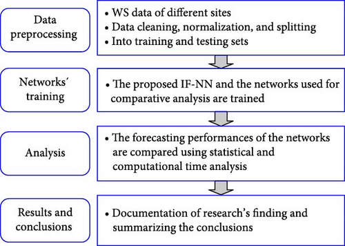
The methodology of the proposed study consists of four steps. The first step deals with data collection and preprocessing, which involves data cleaning, scaling, and splitting. The second step is to train different neural networks for hour-ahead WS forecasting. The statistical performance evaluations and computational time analysis are carried out in step 3. The last step is about reporting and discussing results and summarization of conclusions. In Figure 1, the complete methodology of the proposed study is depicted.
3.1. Spiking Neural Network
State-of-the-art neural networks, including deep learning models, work on the basis of second-generation neurons. These neurons are computationally inefficient. To improve the computational efficiency and minimize power requirements in data-driven modeling, the researcher shifted their attention toward SNNs. The SNNs are made up of third-generations neurons that closely mimic the human biological neurons. These neurons work in discrete events, which reduces the model’s power requirement and computational burden [31]. During the model’s execution, the communication among the neurons is made through spikes that are generated when the firing threshold criteria are met. In this study, we propose an I&F spiking neurons model for WS forecasting.
3.1.1. I&F Neurons
The threshold value is initially set to 0.1, and after the spike emission, the neuron drops its membrane potential and resets itself to Ureset. In our IF-NN network, as in Algorithm 1, we initially set the threshold and reset parameters to 0.1 and 0, respectively. However, these configurations are executed with trainable settings, making these parameters learnable and allowing the network to optimize these values during the training phase. This mechanism allows the neurons to dynamically adjust their firing setting, which improves the IF-NN’s ability to learn the hidden patterns of the datasets. After the two layers of I&F spiking neurons, a dropout layer is added with a dropout rate of 5%. This layer randomly deactivates 5% of the neurons to prevent overfitting of the model. This dropout layer acts as a regularization technique that improves the network’s generalizability by removing its dependencies on specific neurons. Lastly, there is a dense layer with a ReLU activation function that helps the model in capturing the nonlinearities of the data. The IF-NN complied with the Adam optimizer with a learning rate of 0.001, which ensures an effective gradient update during the training process. A loss function is set to MAE, a robust regression performance metric, which monitors the network’s performance during each epoch.
-
Algorithm 1: Proposed IF-NN.
-
Step 01: Importing required packages:TensorFlow, Pandas, Scikit–learn and NumPy
-
Step 02: Load and preprocessing the dataset
-
Dataset reading from the CSV file
-
Normalization through the scaler
-
-
Splitting the data in training, validation, and testing sets with a ratio of 70:10:20
-
Step 03: Define the Spiking Neuron Cell class
-
Inherit from tf.keras.layers.Layer
-
Initialize the number of units and state size
-
Parameter setting of the threshold, reset, and kernel weights
-
Neuron Membrane Potential
-
U(t) = U(t − 1) + I(t).
-
If
-
U(t) ≥ Uthresh,
-
then the spike is emitted,
-
and
-
U(t) ≥ Ureset
-
Else
-
U(t) = U(t)
-
Step 04: Building of the model
-
Define a Sequential model
-
Adding two Spiking Neuron Cell layers
-
Reshaping layer followed by flatten, dropout, and dense layers
-
Step 05: Compiling the model
-
Adam optimizer
-
MAE set as loss function
-
-
Step 06: Training and prediction
-
Train the model using .fit function
-
ypred using .predict function
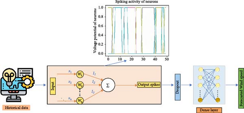
Figure 2 demonstrates that the model starts with processing of historical data by weighing the input features x1, x2, …., xn as W1, W2, ….., Wn as passing them to the summation function Σ, which represents input signals’ integration. The neuron’s membrane potential is analyzed, and the firing of neurons is demonstrated in the spiking activity plot. Then a spiking output is passed to a dropout block illustrating the dropout layer. Finally, there is a fully connected dense layer that performs additional computation on spiking output and provides the final prediction, which is labeled as WS forecast.
3.2. Dataset Description and Preprocessing
The proposed study is tested for the WS datasets of four different locations in KSA. The datasets vary in length and were recorded at intervals of 1 h. The datasets also include other meteorological parameters. The purpose of choosing different lengths of datasets is to find the forecasting stability of the network regarding data points. The datasets are preprocessed in three steps. First, the null values are removed, then data scaling is performed using “MinMax” scaler. Lastly, data splitting is done by dividing the dataset into three subsets: training, validation, and testing. 70% of the data is used for the network’s training. For validation and testing, 10% and 20% of the data are used, respectively.
3.3. Hyperparameters Tuning
The deep learning networks are sensitive to hyperparameters tuning. To fully exploit the deep learning architectures, we tune their hyperparameters through the “Optuna” library. The “Optuna” library is executed for five trials with a defined search space. The optimized value of the hyperparameters with the search space is presented in Table 2. Moreover, this hyperparameter optimization is performed for the Al Jouf location dataset, and the optimized values are also used for other location datasets.
| Model | Hyperparameters | Search space | Optimized value |
|---|---|---|---|
| No. of layers | [2–5] | 2 | |
| No. of units | [32, 64, 96, 128] | 64 | |
| DLN | Learning rate | [0.0001, 0.001, 0.01] | 0.001 |
| Optimizers | [“Adam”, “SGD”, “RMSprop”] | Adam | |
| Dropout | [0.15, 0.2, 0.25] | 0.25 | |
| Batch size | [16, 32] | 32 |
4. Benchmark Techniques
Conventional neural networks have the drawback of retention of information. In the sequential task, the data points share common patterns, and with the inability of the conventional neural networks to store the information, they don’t record better performance. To overcome data retention problems, different deep learning algorithms have been proposed that are made up of second-generation neurons and have layered structures.
4.1. RNN
The RNN can store the information. However, this retention of information is for a short period. Furthermore, the RNN is also affected by the vanishing gradient problem. This gradient problem hinders the updating of the network’s weights and degrades its performance [35]. The issues of vanishing gradient and short-term storage of information lead to the development of different RNN types.
4.1.1. LSTM Network
4.1.2. GRU
4.2. Transformer
A Transformer model has an attention mechanism with parallel operation capability and consists of three layers: self-attention, feedforward, and normalization. The Transformer model has six encoders, and these encoders are identical to each other. The outputs of the encoders are fed to their corresponding decoders. The self-attention and feedforward layers are utilized in the encoder block. The self-attention layer is responsible for finding the relationship among the data points, while the feed-forward layer assists the network for architecture variation regarding the data. The normalization layer uses the softmax activation function for normalizing the score [40].
4.2.1. Informer
For more improved time series forecasting, a variant of the Transformer called Informer was developed. In the Informer architecture, positional encoding information for vector inputs is introduced for better learning of temporal dependencies. The long-term dependency issues are overcome by a multihead attention mechanism. The value to be forecasted is set to 0 to avoid imposing attention on the prior values [42].
4.3. Performance Indicators
The actual and predicted values are denoted by A and B, respectively.
5. Results and Discussion
This section reports the findings of this study. The simulations are performed on the machine with the Intel (R) Core (TM) i5-7200U CPU specification @ 2.50 GHz, 2.70 GHz using Python version 3.10.9. Five libraries: numpy, pandas, matplot, scikit-learn, and TensorFlow are used to implement the networks.
The WS dataset of four locations: Al Jouf, Tuarif, Haffer Al Batin, and Yanbu is used to test the models. The datasets for Al Jouf and Tuarif cities are for 1 year, while for the other two locations, the datasets are for 2 years. Figure 3 illustrates the learning curves of the proposed IF-NN network. The closeness of the training and validation curves illustrates the accurate training of the proposed IF-NN model.
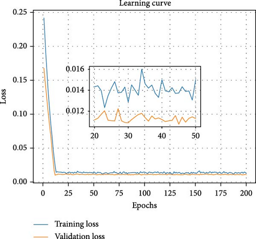
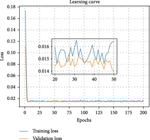
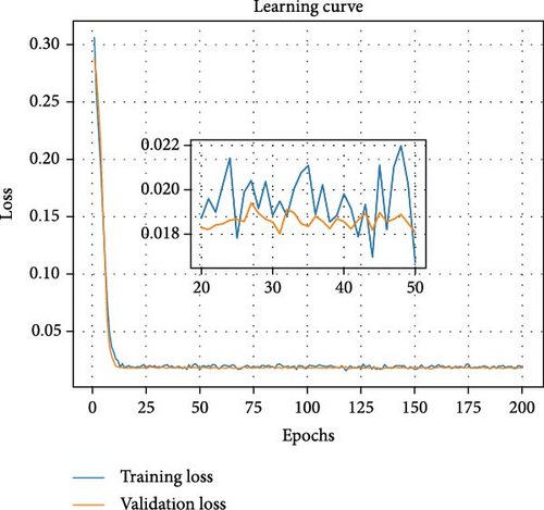
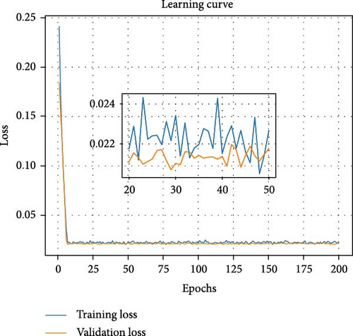
Table 3 reports the forecasting performance of all the networks. The ARIMA and MLR techniques are also used in comparative analysis. These two techniques are classical statistical methods, which are widely used in time series regression problems. In the proposed study, we first analyze the graphs of the autocorrelation function (ACF) and partial correlation function (PCF) to find the possible range of moving average order (q), autoregressive (AR) average (p), and differencing order (d). First, the ARIMA model is iteratively tested on all the possible values of these parameters using a trial-and-error method. The combination that gives the best forecasting performance is selected. The MLR model learns the linear relationship between the target variable and independent external features with weight coefficient optimization for minimizing the loss function, which is MSE. The findings demonstrate that the proposed IF-NN has better forecasting performance than other deep learning networks.
| Location | Models | RMSE | MAE | MAPE | MSE | NRMSE |
|---|---|---|---|---|---|---|
| (m/s) | (m/s) | (%) | (m/s)2 | (%) | ||
| Al Jouf | ARIMA | 2.91 | 2.41 | 60.37 | 8.47 | 45.38 |
| MLR | 2.86 | 2.26 | 51.39 | 8.17 | 48.74 | |
| LSTM | 1.19 | 0.87 | 18.64 | 1.42 | 19.59 | |
| GRU | 1.2 | 0.88 | 18.35 | 1.44 | 19.62 | |
| RNN | 1.22 | 0.88 | 18.37 | 1.49 | 20.28 | |
| Transformer | 1.23 | 0.92 | 20.37 | 1.53 | 20.16 | |
| Informer | 1.3 | 0.97 | 18.94 | 1.7 | 22.92 | |
| RNN-GRU | 1.2 | 0.89 | 18.04 | 1.46 | 20.39 | |
| RNN-LSTM | 1.18 | 0.85 | 17.91 | 1.39 | 19.59 | |
| CNN-LSTM | 1.26 | 0.93 | 21.41 | 1.58 | 20.07 | |
| IF-NN | 0.32 | 0.29 | 4.6 | 0.1 | 5.54 | |
|
ARIMA | 3.43 | 2.85 | 66.01 | 11.78 | 45.26 |
| MLR | 3.41 | 2.81 | 64.44 | 11.61 | 42.91 | |
| LSTM | 1.16 | 0.85 | 15.71 | 1.35 | 16.16 | |
| GRU | 1.2 | 0.87 | 16.02 | 1.45 | 16.54 | |
| RNN | 1.17 | 0.87 | 16.42 | 1.37 | 16.43 | |
| Transformer | 1.3 | 0.99 | 21.09 | 1.69 | 17.12 | |
| Informer | 1.24 | 0.92 | 17.19 | 1.54 | 17.46 | |
| RNN-GRU | 1.16 | 0.85 | 16.09 | 1.35 | 16.07 | |
| RNN-LSTM | 1.16 | 0.85 | 16.47 | 1.35 | 16.05 | |
| CNN-LSTM | 1.14 | 0.83 | 15.58 | 1.31 | 15.82 | |
| IF-NN | 0.38 | 0.34 | 4.69 | 0.14 | 5.58 | |
| Turaif | ARIMA | 3.24 | 2.70 | 66.17 | 10.53 | 42.82 |
| MLR | 2.94 | 2.39 | 49.76 | 8.64 | 44.72 | |
| LSTM | 1.23 | 0.94 | 15.99 | 1.52 | 18.68 | |
| GRU | 1.14 | 0.86 | 16.32 | 1.3 | 16.15 | |
| RNN | 1.13 | 0.86 | 16.58 | 1.28 | 15.69 | |
| Transformer | 1.21 | 0.92 | 17.07 | 1.45 | 17.54 | |
| Informer | 1.24 | 0.95 | 19.66 | 1.54 | 17.03 | |
| RNN-GRU | 1.17 | 0.88 | 15.5 | 1.39 | 17.47 | |
| RNN-LSTM | 1.12 | 0.84 | 15.27 | 1.27 | 16.04 | |
| CNN-LSTM | 1.16 | 0.88 | 17.22 | 1.36 | 16.77 | |
| IF-NN | 0.37 | 0.33 | 4.76 | 0.14 | 5.57 | |
| Yanbu | ARIMA | 3.98 | 3.28 | 65.48 | 15.85 | 42.39 |
| MLR | 3.27 | 2.65 | 48.49 | 10.70 | 34.75 | |
| LSTM | 1.18 | 0.86 | 14.12 | 1.39 | 13.6 | |
| GRU | 1.15 | 0.83 | 14.28 | 1.31 | 12.88 | |
| RNN | 1.18 | 0.86 | 15.33 | 1.39 | 12.96 | |
| Transformer | 1.23 | 0.91 | 14.71 | 1.52 | 14.32 | |
| Informer | 1.38 | 1.03 | 16.66 | 1.91 | 14.82 | |
| RNN-GRU | 1.17 | 0.86 | 15.36 | 1.38 | 12.92 | |
| RNN-LSTM | 1.15 | 0.83 | 14.02 | 1.33 | 13.13 | |
| CNN-LSTM | 1.12 | 0.82 | 13.95 | 1.26 | 12.7 | |
| IF-NN | 0.46 | 0.42 | 4.73 | 0.21 | 5.56 | |
- Note: The blod italic values is to highlight our work.
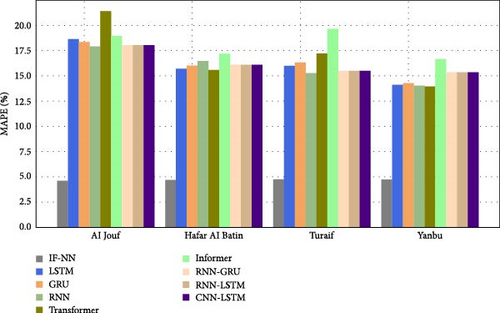
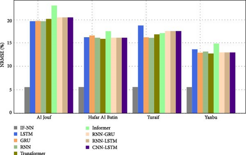
For the Al Jouf site, the IF-NN records the RMSE, MAE, MAPE, MSE, and NRMSE of 0.32%, 0.29%, 4.6%, 0.1%, and 5.54%, respectively. In the case of Haffer Al Battin site, the RMSE, MAE, MAPE, MSE, and NRMSE of IF-NN are 0.38%, 0.34%, 4.69%, 0.14%, and 5.58%, respectively. For the Turaif WS dataset, the IF-NN records the RMSE, MAE, MAPE, MSE, and NRMSE of 0.37%, 0.33%, 4.76%, 0.14%, and 5.57%, respectively. In the case of Yanbu site, the recorded RMSE, MAE, MAPE, MSE, and NRMSE of the IF-NN are found to be 0.46%, 0.42%, 4.73%, 0.21%, and 5.56%, respectively. In Figure 4, the MAPE and NRMSE of the IF-NN and the networks used for comparative analysis are depicted as bar plots.
To demonstrate the robustness of IF-NN for hour-ahead WS forecasting, Figure 5 compares the forecasted curves of IF-NN with the measured WS curves.
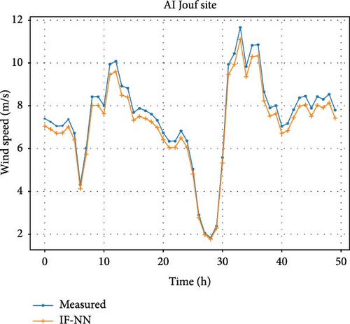
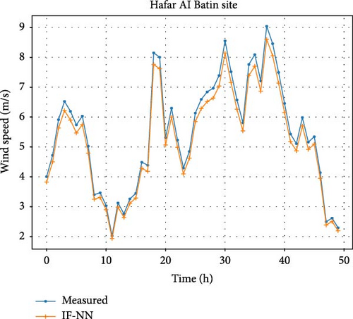
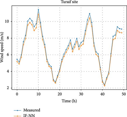
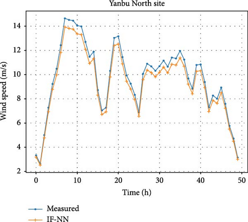
The accurate fitting of the forecasted curves illustrates the effectiveness of IF-NN in hour-ahead WS forecasting. The SNNs work in a binary way, which makes them computationally efficient algorithms. To validate this aspect, we compare the computational time recorded by the IF-NN with other deep learning networks. In Table 4, the computational time recorded by each network is reported.
| Location | Models | Convergence | Inference | Computational |
|---|---|---|---|---|
| (s) | (s) | (s) | ||
| Al Jouf | LSTM | 466.98 | 2.03 | 469.01 |
| GRU | 454.67 | 1.47 | 456.14 | |
| RNN | 236.61 | 0.64 | 237.25 | |
| Transformer | 328.98 | 1.11 | 330.09 | |
| Informer | 448.49 | 1.55 | 450.04 | |
| RNN-GRU | 370.29 | 0.98 | 371.27 | |
| RNN-LSTM | 502.09 | 0.86 | 502.95 | |
| CNN-LSTM | 422.21 | 2.01 | 424.22 | |
| IF-NN | 109.58 | 0.29 | 109.87 | |
| Hafar Al Batin | LSTM | 904.25 | 6.69 | 910.94 |
| GRU | 890.46 | 1.82 | 892.28 | |
| RNN | 448.82 | 1.29 | 450.11 | |
| Transformer | 662.4 | 1.98 | 664.38 | |
| Informer | 709.69 | 1.69 | 711.38 | |
| RNN-GRU | 764.09 | 1.13 | 765.22 | |
| RNN-LSTM | 772.69 | 1.3 | 773.99 | |
| CNN-LSTM | 598.48 | 1.44 | 599.92 | |
| IF-NN | 211.84 | 0.63 | 212.47 | |
| Turaif | LSTM | 422.8 | 1.56 | 424.36 |
| GRU | 434.58 | 2.89 | 437.47 | |
| RNN | 228.25 | 0.88 | 229.13 | |
| Transformer | 277.16 | 1.26 | 278.42 | |
| Informer | 318.98 | 2.35 | 321.33 | |
| RNN-GRU | 353.39 | 0.85 | 354.24 | |
| RNN-LSTM | 363.64 | 1.13 | 364.77 | |
| CNN-LSTM | 308.36 | 1.82 | 310.18 | |
| IF-NN | 105.29 | 0.36 | 105.65 | |
| Yanbu | LSTM | 951.25 | 2.02 | 953.27 |
| GRU | 895.18 | 1.8 | 896.98 | |
| RNN | 523.68 | 0.88 | 524.56 | |
| Transformer | 649.41 | 1.83 | 651.24 | |
| Informer | 689.46 | 1.5 | 690.96 | |
| RNN-GRU | 864.23 | 2.03 | 866.26 | |
| RNN-LSTM | 662.25 | 1.12 | 663.37 | |
| CNN-LSTM | 902 | 1.82 | 903.82 | |
| IF-NN | 205.11 | 0.6 | 205.71 | |
- Note: The blod italic values is to highlight our work.
The findings illustrate that the IF-NN has less computational time than other deep learning networks. In Figure 6, the computational time comparison is demonstrated with a bar plot.
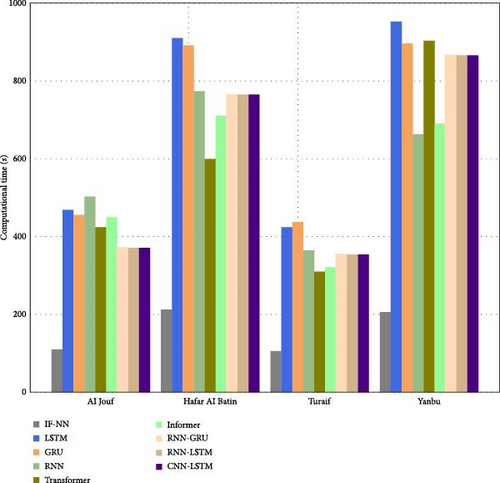
One of the contributing points of the proposed study is to evaluate the impact of dataset points on the performance of the models. The findings of Table 3 demonstrate that, unlike the conventional deep learning methods, the proposed IF-NN records consistent forecasting performance irrespective of data points. This highlights the robustness of the IF-NN for WS forecasting in the realm of limited data.
The comparative analysis performed in this study reveals that the proposed IF-NN has better forecasting performance than other cutting-edge deep learning networks. Moreover, the findings also demonstrate that the deep learning networks require more data points for improved forecasting outcomes, while the spiking neurons-based proposed approach records similar performance with reduced computational overhead regardless of dataset lengths. This superior performance of the IF-NN is due to spiking neurons. These neurons mimic the human biological neurons and learn the temporal dependencies of the dataset effectively. Moreover, the binary nature-based working of these neurons reduces the computational burden of the network. Thus, the proposed study offers a unique network for improved WS forecasting with efficient computational characteristics, especially in the scenario of limited available data.
6. Conclusions
In this proposed study, we have presented a third-generation neuron model, IF-NN, for short-term forecasting of WS. The datasets of four different locations of KSA are used for simulation. The proposed approach leverages the advantages of I&F spiking neurons for learning the inherent data patterns. These neurons closely relate to human biological neurons, and the binary functionality of these neurons reduces the computational overhead of the network. To demonstrate the scalability and robustness of the proposed IF-NN approach for WS forecasting, its performance is compared with state-of-the-art deep learning networks. Findings illustrate that for the datasets of Al Jouf and Turaif cities, the proposed model records an improvement of 74.3% and 68.8% in MAPE as compared to RNN-LSTM, which was found to be the second-best performing model for these datasets. While for Haffer Al Batin and Yanbu datasets, the MAPE of IF-NN is 69.9% and 65.9% better than the MAPE of CNN-LSTM, which records the second-best forecasting performance among the models used for comparative analysis. In the proposed study, the computational time comparison of the models is also performed. Results illustrate that for each dataset, IF-NN has better computational time as compared to RNN due to spiking neurons. Therefore, this study provides a novel approach for efficient WS forecasting with better computational properties, particularly in the case of limited accessible data.
Nomenclature
-
- AdaBoost:
-
- Adaptive boosting
-
- AFNN:
-
- Adaptative fuzzy neural network
-
- AI:
-
- Artificial intelligence
-
- ANN:
-
- Artificial neural network
-
- AR:
-
- Autoregressive
-
- ARIMA:
-
- Autoregressive integrated moving average
-
- ARMA:
-
- Autoregressive moving average
-
- BiLSTM:
-
- Bidirectional long short-term memory network
-
- BPNN:
-
- Back-propagation neural networks
-
- CatBoost:
-
- Categorical boosting
-
- CNN:
-
- Convolutional neural network
-
- ES:
-
- Exponential smoothing
-
- FFNN:
-
- Feed forward neural network
-
- GA:
-
- Genetic algorithm
-
- GB:
-
- Gradient boosting
-
- GRU:
-
- Gated recurrent unit
-
- IEA:
-
- International energy agency
-
- KNN:
-
- k-nearest neighbor
-
- LGBM:
-
- light gradient boosting machine
-
- LSTM:
-
- Long short-term memory network
-
- MAE:
-
- Mean absolute error
-
- MAPE:
-
- Mean absolute percentage error
-
- MASE:
-
- Mean absolute scaled error
-
- MBE:
-
- Mean bias error
-
- MC:
-
- Markov chain
-
- MSE:
-
- Mean square error
-
- NSRDB:
-
- National solar radiation database
-
- PCC:
-
- Pearson correlation coefficient
-
- RF:
-
- Random rorest
-
- RMSE:
-
- Root mean square error
-
- SGD:
-
- Stochastic gradient decent
-
- SVM:
-
- Support vector machine
-
- VREI:
-
- Variable renewable energy integrating
-
- XgBoost:
-
- Extreme gradient boosting.
Ethics Statement
The authors have nothing to report.
Consent
The authors have nothing to report.
Conflicts of Interest
The authors declare no conflict of interest.
Funding
The Researchers would like to thank the Deanship of Graduate Studies and Scientific Research at Qassim University for financial support (QU-APC-2025).
Acknowledgments
The authors declare that they did not use Generative AI and AI-assisted technologies to prepare the whole manuscript and its sections.
Open Research
Data Availability Statement
The datasets of solar irradiation utilized in this study were recorded from solar monitoring stations in Riyadh, Saudi Arabia, and were provided by the King Abdullah City for Atomic and Renewable Energy (K.A. CARE). K.A. CARE is a leading organization in Saudi Arabia dedicated to advancing renewable energy research and development. The datasets are not publicly available, but can be requested directly from K.A. CARE, subject to their data-sharing policies and approval.


