The presence of offshore wind farms (OWFs) reduces the inertia of the power system and jeopardizes its frequency stability. Considering virtual inertia control (VIC) for these farms improves the frequency stability and inertia in the power system. In this paper, the robust H∞ controller based on deep reinforcement learning (DRL) is designed to improve the frequency stability in the load–frequency control (LFC) of the power system by considering the effect of OWFs on frequency control. The proposed method is robust to disturbances (load and wind fluctuations) and uncertainties related to system parameters and can adapt to uncertainties. The robust H∞ controller is designed based on linear matrix inequality (LMI) and DRL optimizes the robust H∞ controller and will improve the overall performance of the system. To examine the performance of the proposed method (H∞–DRL), several scenarios have been considered and compared with DMPC and PID control methods. The results show the superiority of the proposed method, which has been able to reduce load and wind fluctuations, frequency deviations, and also power deviations of the tie-line between the lines of the multi-area power system.

1. Introduction

Owing to the potential for strong and steady winds, offshore wind farms (OWFs) are regarded as one of the most significant sources of clean energy and one of the most significant renewable energy sources [1–3]. OWFs provide a number of benefits, including as better utilization of marine resources, more steady and greater energy production, and less noise pollution because they are located far from land regions [4–6]. The presence of OWFs in the power system also has challenges [7]. One of the most important challenges is that these farms use induction generators instead of synchronous generators, which makes the farms unable to provide natural inertia [8]. The inability of OWFs causes the performance of the load–frequency control (LFC) in the power system to be compromised in the presence of these farms, and frequency fluctuations as well as power fluctuations between tie-lines in the power system increase [9]. By modeling the behavior of mechanical inertia, virtual inertia control (VIC) design for these farms enhances the power system’s frequency stability [10].

In [11, 12], to improve the frequency stability of the power system along with the LFC, the concept of VIC for OWFs has been proposed. When the power signal and the maximum efficiency tracking signal are combined in [13], the WTs actively take part in the system’s frequency regulation. In [14–16], VIC on OWFs based on the proportional–derivative method (VIC and VDC) is proposed. The larger the VDC gain and VIC in OWFs, the more kinetic energy will be released from the rotor, which will improve the frequency stability [17]. The value of the VDC gain and the VIC gain depends on the rotor speed, and if these values are considered large, it may cause the rotor speed to go out of the operating range and lead to system instability [18]. Therefore, the presence of VIC and VDC for OWFs along with the LFC in the power system seems essential. Several control methods have been considered to improve the LFC in the power system with the presence of OWFs and the advantages and disadvantages of each are fully stated in Table 1 for reference.

Table 1. Advantages and disadvantages of control techniques implemented on LFC in the presence of the OWFs.

Methodologies employed	Main findings	Deficiency of the method used
Cascaded FOPD–FOPID controller based on DOSA [19]	Increasing the frequency stability of the power system when there are disruptions and system unpredictability	OWFs do not participate in power system frequency control, not resistant to severe disturbances
Robust fuzzy controller [20]	Enhancing a power system’s frequency deviations to make it more resilient to minor disruptions and moderate parameter uncertainties	Inadequate resilience to significant disruptions and significant ambiguity surrounding the boundaries of the power system, OWFs do not participate in power system frequency control
FOPID–TID controller [21]	Increasing the frequency stability of the power system when there are disruptions and system unpredictability	OWFs do not participate in power system frequency control, not resistant to severe disturbances
FMPC controller [22]	Lower frequency deviations, increase the power system’s stability, and withstand small uncertainties in the parameters of the power system	Insufficient resilience to significant disruptions and significant ambiguity surrounding the system’s specifications, OWFs do not participate in power system frequency control
Fuzzy PID controller [23]	Enhancing a power system’s frequency deviations to make it more resilient to minor disruptions and moderate parameter uncertainties	Inadequate resilience to significant disruptions and significant ambiguity surrounding the boundaries of the power system, OWFs do not participate in power system frequency control
PI^λ (1+PDF) controller [24]	Increasing the frequency stability of the power system when there are disruptions and system unpredictability	OWFs do not participate in power system frequency control, not resistant to severe disturbances
3DOF–PID controller [25]	Increasing the frequency stability of the power system when there are disruptions and system unpredictability	OWFs do not participate in power system frequency control, not resistant to severe disturbances
SMC controller [26, 27]	Reduce frequency deviations, improve power system stability, resistant to mild disturbances, and mild uncertainty related to system parameters	Chattering phenomenon (high frequency oscillations) during severe disturbances
MPC controller [28, 29]	Lower frequency deviations, increase the power system’s stability, and withstand small uncertainties in the parameters of the power system	Insufficient resilience to significant disruptions and significant ambiguity surrounding the system’s specifications
DMPC controller [30]	Lower frequency deviations, increase the power system’s stability, and withstand small uncertainties in the parameters of the power system	Insufficient resilience to significant disruptions and significant ambiguity surrounding the system’s specifications

Given the drawbacks listed in Table 1, a suitable method for the power system’s LFC must be designed, taking into account the impact of OWFs in frequency control. This method must be both resilient to disturbances and uncertainties pertaining to the power system’s parameters and flexible enough to adjust to system uncertainties. The robust H∞ controller is designed to establish power system stability, resistant performance against wind, and load fluctuations as well as uncertainties related to the system parameters. This controller might not react to uncertainties outside of the specified range and might not operate at its best since it is made for a certain set of power system uncertainties. On the other hand, the robust H∞ controller is strongly dependent on the accurate state space model of the power system, which is usually not available in many cases. Therefore, the robust H∞ controller is designed based on deep reinforcement learning (DRL), which has several advantages, including:

•
DRL is a data-driven and adaptive method that can reduce the access limitations of the H∞ robust controller in terms of access to the complete model and adapt itself to the changing conditions of the power system.
•
Given that in this paper, the FNN is used in the DRL structure, which ensures the conditions of the H∞ robust controller and also leads to the creation of an optimal controller for LFC of the power system.
•
DRL will continuously improve the performance of the robust controller in the LFC of the power system.

By taking into account the impact of OWFs on frequency management, the robust H∞ controller based on DRL is built in this study to enhance frequency stability in the power system. The suggested approach can adjust to uncertainties and is resilient to disturbances (load and wind variations) and uncertainty pertaining to system parameters. Linear matrix inequality (LMI) serves as the foundation for the robust H∞ controller’s design and DRL improves it to boost system performance as a whole. A number of situations have been examined and contrasted using DMPC and PID control methods in order to examine the effectiveness of the suggested approach. The outcomes demonstrate how effective the suggested approach is at mitigating load and wind changes by lowering the frequency and power deviations of the tie-line connecting the lines of the multi-area power system. Generally speaking, this paper’s contributions consist of the following:

•
Combining H∞ controller with DRL to improve the LFC problem in the power system considering the effect of OWFs on frequency control: In this paper, instead of numerical solution methods used for designing robust control, DRL is used for its design.
•
Converting the H∞ controller to LMI and using LMI in calculating the reward in DRL.
•
Online learning of the robust controller in the presence of disturbances and uncertainty of power system parameters.
•
Using a neural network to predict the H∞ controller.
•
Multiobjective optimization: DRL allows the agent to simultaneously optimize multiple objectives (satisfying the conditions of the H∞ robust controller, optimizing the performance of H∞, etc.)

The structure of the paper consists of several sections. Section 2 presents the dynamic model of the power system considering the effect of OWFs on frequency control. In Section 3, the proposed controller is designed. Sections 4 and 5 present the simulation and results, respectively.

2. The Dynamic Model of Power System Considering the Effect of OWFs in Frequency Control

2.1. The Model of OWFs in Frequency Control

The following phases are included in OWFs, which are made up of many WTs that transform wind energy into mechanical and electrical energy.

2.1.1. Conversion of Wind Energy Into Mechanical Power

Wind energy will be converted into mechanical energy by the blades in the WTs. Equation (1) illustrates the mechanical power that the wind provides [11, 12].

(1)

In Equation (1), P_m (mechanical power of WTG): the mechanical power extracted from the wind by the turbine blades; C_p (power coefficient): represents the efficiency of the wind energy conversion process; λ (tip-speed ratio): the ratio of the blade tip speed to the wind speed, which affects power efficiency; β: the angle of the turbine blades, which controls power extraction; ρ: the density of air; r: radius of the wind turbine blades; v: wind speed.

2.1.2. Transferring Mechanical Power to the Generator

Then, the mechanical power is transmitted to a generator through the transmission system according to Equation (2) [30].

(2)

In Equation (2), ΔT = P_m − P_e/ω, F: friction coefficient of the transmission system, P_e: output of the generator of WTG, ω: rotor speed of WTG, and H_w: inertia coefficient of transmission system of WTG.

2.1.3. MPPT

The WTG should operate at its maximum power in ideal conditions and a method called MPPT is used to adjust the optimal power in the WTs according to Equation (3) [17, 30].

(3)

In Equation (3), K_c: maximum power tracking coefficient of WTG, ω_n: rated rotor speed, and P_ω: the optimal power in the WTs.

2.1.4. Dynamic Modeling of VIC and VDC in WTs

Considering the VIC of OWFs, the reference power of the inverter of WTG includes MPPT power and VIC power. Therefore, the electromagnetic power output of OWFs is shown according to Equation (4) [13, 30].

(4)

In Equation (3), ΔP_f = −(K_Ds + K_p)Δf, K_D: VIC gain, K_P: virtual damping gain, T_e: time constant of generator of WTG, and P_e: the electromagnetic power output of OWFs.

2.2. The TPP Modeling

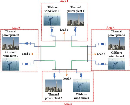
TPPs, which supply electricity and regulate the frequency in this system, are among the most crucial parts of the power system [29, 30]. The components of TPPs that are modeled for frequency stability include the Governor model, the Boiler model, the turbine model, and the frequency regulation model. In this paper, the power system is considered to consist of four areas as shown in Figure 1, each area including TPPs and OWFs [29, 30]. In Figure 2, the dynamic model of the power system including TPPs and OWFs is shown by considering VIC and VDC on these farms for one area [28–30]. This dynamic model is a first-order (reduced order) model for the power system components, which is a suitable model for frequency stability analysis. The parameters related to the power system are given in Table A1 [28–30].

Details are in the caption following the image — **Figure 1**
Open in figure viewer PowerPoint

The power system consists of four areas [29, 30].

2.3. The State–Space Model of the Power System and OWFs for Each Area

The state–space model of the OWFs and power system for each region is presented in Equation (5) [29, 30]. The matrices associated with the power system’s state–space are specified in Equation (6):

(5)

(6)

3. Design of the Proposed Controller

3.1. H∞ Controller

The H∞ controller is a robust design method for dynamic systems that aims to reduce the system’s sensitivity to external disturbances and model uncertainties. This controller is designed by solving LMI. The H∞ controller has two main objectives: (1) The power system must remain stable in the presence of disturbances and system-related uncertainties. (2) The energy bound of the power system response to external disturbances is minimized. The state–space model for each area of the power system is shown in Equation (7) [31–33].

(7)

In Equation (7), A, B, C, D, B_ω, and D_ω are the nominal matrices of the power system and ΔA, ΔB, ΔC, and ΔD are the uncertainties related to the power system. Also, ω is the external disturbances entering the power system and z is the desired output. The uncertainties related to the model are shown in the form of a box according to Equation (8).

(8)

The scope of parameter uncertainty is defined as follows:

Uncertainty in system inertia (M_i): The system inertia can change due to changes in the system load or changes in the number of generators connected to the system. In this paper, the uncertainty in system inertia is considered as (±20%) of the nominal value.

Uncertainty in damping coefficient (D_i): The damping coefficient of the system can also change due to changes in the system load or changes in environmental conditions. In this paper, the uncertainty in the damping coefficient is considered as (±20%) of the nominal value.

In Equation (8), H and E are constant matrices and Θ is an indefinite matrix obtained according to Equation (9):

(9)

To ensure robust stability of the H∞ control (K), there must be a Lyapunov matrix P > 0 that satisfies Equation (10).

(10)

Also, the transfer gain ω to z must be bounded according to Equation (11).

(11)

In order to convert Equations (10) and (11) into LMI, the S-Procedure lemma has been used, and finally the form of Equations (12) and (13) has been shown.

(12)

(13)

Solving the LMI associated with the H∞ controller (Equation (13)) can be complex and time-consuming and this robust H∞ controller cannot adapt adaptively to environmental changes. DRL is used in this paper to learn the H∞ control policy adaptively and online. On the other hand, this method models the changes caused by uncertainty and disturbances well. DRL controls the performance of H∞ and robust stability together.

3.2. RL

RL is an important branch of machine learning that aims to train an agent to make optimal decisions in an environment [34]. In this method, the agent learns an optimal policy to maximize long-term reward through interaction with the environment and specifically through trial and error. The following describes the principles of reinforcement learning and its details, including the Q-learning method used in this article.

In RL, the agent continuously moves in the environment, observes states, selects actions, and receives rewards in return [35–37]. The main goal of RL is to find a policy that selects the best possible action in each case to receive the highest reward. The main components of RL include the following:

•
Agent: A decision-maker who takes action in the environment.
•
Environment: The system in which the agent operates and which provides responses such as state changes and rewards to the agent.
•
States (s): The states that the environment can be in. The states of the system are described in terms of state variables and are discretized for simplicity.
•
Actions (a): A set of inputs or controls that the agent can perform. In this paper, inputs are chosen as discrete values over a range of continuous values.
•
Reward (r): A signal that the environment gives the agent for each action to evaluate the quality of its performance.
•
Policy (π(a|s)): A rule or strategy that the agent uses to make a decision in each state.

In RL, the strategy is that the agent has used to select actions a in state s according to Equation (14) [34, 35].

(14)

In Equation (14), π(a|s) is the probability of choosing action a in state s.

The state–action value function, defined according to Equation (15), can evaluate the quality of the state–action [34, 35].

(15)

In RL, the policy is updated in a way that optimizes the cumulative return according to Equation (16) [34, 35].

(16)

In RL, the value function is updated based on the policy gradient or Q-learning according to Equation (17) [34, 35].

(17)

In Equation (17), r represents the reward for the quality of action a in state s, Λ is the discount rate, which has a value between zero and one.

3.3. DRL

It is an improved version of RL in which the neural network extracts more complex features from the training data that perform better in new environments. Also, in this paper, the reward is based on the robust stability criterion and the LMI error reduction, so DRL can better model complex rewards and learn policies that optimize this robust controller criterion H∞.

The neural network is used to approximate the policy or value function in DRL according to Equation (18).

(18)

In Equation (18), θ are the weights of the neural network.

Using the reward gradient, the neural network parameters will be updated according to Equation (19).

(19)

In Equation (19), J(π_θ) is the objective function defined as a cumulative reward and needs to be optimized.

The policy gradient is calculated using Equation (20).

(20)

In DRL, the value function Q(s, a) is approximated by a neural network according to Equation (21) and its updating is done by Equation (22).

(21)

(22)

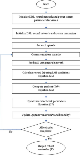
3.4. Design of H∞ Robust Controller Based on DRL

In DRL for this paper, the state vector of each area’s power system (x) is considered as the state (s) that describes the current state of the system. The robust controller matrix (K) predicted by the neural network is considered as the action (a) in DRL. A function that evaluates the quality of the controller K is considered as the reward (r) for DRL. The dynamic system of each area of the power system is used as the environment and the neural network with the parameter θ that models the mapping between state s and action a is used as the policy in DRL. The following are the steps of designing the H∞ controller based on DRL:

1.
In this learning stage, a random state x is generated from the power system state-space of each area according to Equation (23).

(23)

2.
At this stage, the neural network π_θ predicts the matrix corresponding to the robust controller (K) by receiving the state x of the power system according to Equation (24).

(24)

3.
After obtaining K, the robust stability condition and the performance of H∞ should be evaluated. The reward function is defined as Equation (25). The goal of this reward function is to improve the LMI condition and minimize the values of trace (P) and γ². In Equation (25), decreasing r means improving the robust controller.

(25)

In Equation (25), trace (P) is considered as a criterion for reducing the system energy and its stability. The Frobenius norm LMI is the LMI condition which must be negative. LMI is referred to in Equation (13) and γ² is the robust control performance bound H∞.

4.
In order to update the FNN parameters, the gradient of the reward function with respect to the FNN parameters θ is calculated according to Equation (26).

(26)

5.
Using the gradient and the learning rate α, the neural network parameters are updated according to Equation (27).

(27)

Updating the neural network parameters according to Equation (27) improves the policy π_θ and produces a more optimal controller. Figure 3 displays the suggested method’s flowchart. Table 2 displays the suggested method’s beginning settings. Table 3 displays the pseudocode for the suggested approach.

Table 2. The initial parameters of the proposed method.

Parameter	Value	Parameter	Value
n (Number of system states)	7	Θ	I₇: Initial Lyapunov matrix

m (Number of control inputs)	1	γ	10

q (Number of system outputs)	1	Input layer (neural network)	7 (the number of system states)

p (Number of external disturbances)	1	Hidden layers (neural network)	1 (64 neurons)

H (Uncertainty matrix)	Uncertainty matrix (7 × 7)	Output layer (neural network)	7 (the dimensions of the control matrix K)

E (Uncertainty matrix)	Uncertainty matrix (7 × 7)	Learning rate (α) (reinforcement learning)	0.01

P	I₇: Initial Lyapunov matrix	Number of episodes (reinforcement learning)	500

Table 3. The pseudocode of the proposed method.

clc; clear; close all;
% 1. Define the system
n = … m = … q = … p = …
A = …
B = …
C = …;
D = …
D_w = …
B_w = …
% Define uncertainties
H = randn (n, n);
E = randn (n, n);
% 2. Initial parameters
P = eye (n); % Lyapunov matrix
Theta = eye (n); % Uncertainty parameter
gamma = 10; % H-infinity bound
% 3. Deep reinforcement learning settings
episodes = 500;
alpha = 0.01; % Learning rate
hidden_units = 64; % Number of hidden layer neurons
% Define a custom neural network
layers = [
featureInputLayer (n, ‘Name’, ‘state_input’)
fullyConnectedLayer (hidden_units, ‘Name’, ‘fc1’)
reluLayer (‘Name’, ‘relu1’)
fullyConnectedLayer (m ^∗ n, ‘Name’, ‘fc2’) % Output dimensions for K
];
net = dlnetwork (layers);
% 4. Deep Reinforcement Learning Loop
for ep = 1:episodes
% Generate a random state
x = randn (n, 1); % Random system state
dlX = dlarray (x, ‘CB’); % Convert to neural network format
% Compute gradients and reward
[grad, reward] = dlfeval (@modelGradient, net, dlX, P, A, B, C, D, B_w, D_w, gamma);
% Update the network
net.Learnables = dlupdate (@ (w, g) w - alpha ^∗ g, net.Learnables, grad);
% Update system parameters
P = P + alpha ^∗ eye (n); % Update P
gamma = max (gamma - alpha, 1); % Decrease gamma
Theta = Theta - alpha ^∗ eye (n); % Decrease uncertainty
% Display results every few episodes
if mod (ep, 50) = = 0
fprintf (‘Episode %d: Reward = %.2f, Gamma = %. 2f\n’, ep, extractdata (reward), gamma);
end
end
disp (‘Final robust controller:’);
K = extractdata (grad); % Final computed controller
disp (K);
% 5. Gradient and Reward Function
function [grad, reward] = modelGradient (net, dlX, P, A, B, C, D, B_w, D_w, gamma)
% Predict controller K from the network
dlU = forward (net, dlX); % Predict controller
u = extractdata (dlU); % Convert to numeric data
K = reshape (u, [size (B, 2), size (A, 1)]); % Reshape output to controller matrix
% Compute reward
LMI = [A’ ^∗ P + P ^∗ A + B ^∗ (K ^∗ P) + (K ^∗ P)’ ^∗ B’ + H ^∗ P ^∗ H’, P ^∗ C’ + (K ^∗ P)’ ^∗ D’, B_w;
C ^∗ P + D ^∗ K ^∗ P, -gamma 2 ^∗ eye(size (C, 1)), D_w;
B_w’, D_w’, -eye(size (B_w, 2))];
reward = -trace (P) - gamma² - norm (LMI, ‘fro’); % Reward based on conditions
% Convert reward to dlarray
reward = dlarray (reward, ‘CB’);
% Compute gradients with respect to network parameters
grad = dlgradient (reward, net.Learnables);
end

4. Simulation

Parameters related to the multi-area power system are included in Table A1. In order to compare the proposed method (H∞–DRL) in the LFC structure of the power system considering the effect of OWFs on frequency control, three scenarios are considered and compared with DMPC and PID control methods. Using various control techniques, the impact of minor disruptions on the multi-area power system is examined in Scenario (1). In Scenario (2), several control techniques are used to examine the impact of moderate disruptions and mild uncertainty pertaining to the multi-area power system’s characteristics. In Scenario (3), several control techniques are used to examine the impact of severe disruptions and severe uncertainty pertaining to the multi-area power system’s characteristics.

4.1. Scenario (1)

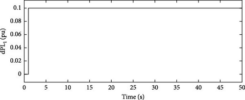
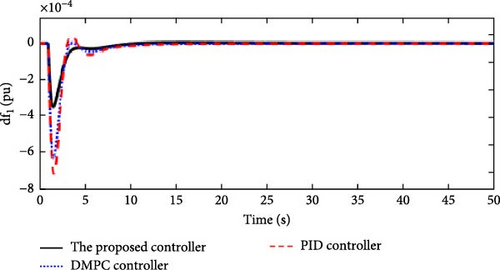
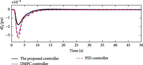
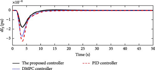
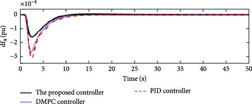
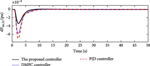
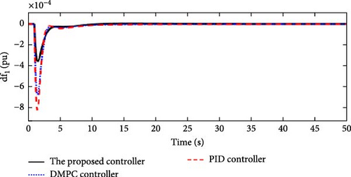
In this scenario, a load disturbance is introduced into Area 1 of a multi-area power system as shown in Figure 4. Figures 5, 6, 7, and 8 show the FDs of Areas 1, 2, 3, and 4 using different control methods, respectively. Figures 9, 10, 11, and 12 show the PDs of the tie-line for Areas 1–2, 2–3, 3–4, and 4–1 using different control methods, respectively. According to Figures 5–12, the proposed control method (H∞–DRL) has been able to reduce the FDs as well as the PDs between the tie-lines and has an effective performance against mild disturbances. The proposed method has also been able to suppress the oscillations in a shorter time. The results of Scenario (1) are shown in Tables 4 and 5.

Table 4. Results for Scenario (1) FDs.

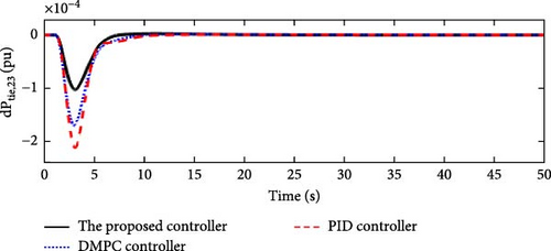
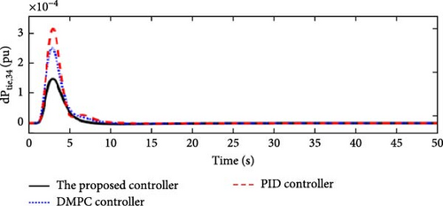
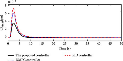
Controller	Δf₁(pu)			Δf₂(pu)			Δf₃(pu)			Δf₄(pu)
Controller	MO (pu)	MU (pu)	ST (s)	MO (pu)	MU (pu)	ST (s)	MO (pu)	MU (pu)	ST (s)	MO (pu)	MU (pu)	ST (s)
The proposed controller	0	3 × 10⁻⁴	9	0	1.7 × 10⁻⁴	9	0	1.5 × 10⁻⁴	10	0	1.5 × 10⁻⁴	10
DMPC controller	0	6 × 10⁻⁴	11	0	3 × 10⁻⁴	11	0	2.8 × 10⁻⁴	11	0	2.8 × 10⁻⁴	11
PID controller	1 × 10⁻⁴	7 × 10⁻⁴	13	0	3.5 × 10⁻⁴	13	0	3.3 × 10⁻⁴	14	0	3.3 × 10⁻⁴	14

Table 5. Results for Scenario (1) PDs.

Controller	ΔP_tie,12(pu)			ΔP_tie,23(pu)			ΔP_tie,34(pu)			ΔP_tie,41(pu)
Controller	MO (pu)	MU (pu)	ST (s)	MO (pu)	MU (pu)	ST (s)	MO (pu)	MU (pu)	ST (s)	MO (pu)	MU (pu)	ST (s)
The proposed controller	0	3 × 10⁻⁴	9	0	1.1 × 10⁻⁴	7	1.5 × 10⁻⁴	0	8	3.8 × 10⁻⁴	0	8
DMPC controller	0	5.8 × 10⁻⁴	11	0	1.8 × 10⁻⁴	10	2.5 × 10⁻⁴	0	10	6 × 10⁻⁴	0	10
PID controller	1 × 10⁻⁴	6.5 × 10⁻⁴	13	0	2.2 × 10⁻⁴	12	3.3 × 10⁻⁴	0	12	7.2 × 10⁻⁴	0	13

4.2. Scenario (2)

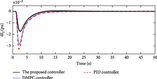
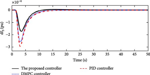
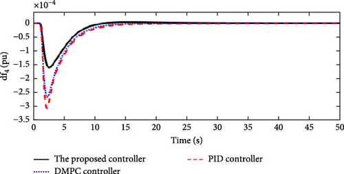
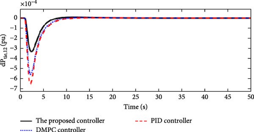
In this scenario, a load disturbance is introduced into Area 1 of a multi-area power system as shown in Figure 4. Also, in this scenario, the effect of slight uncertainties in the parameters D and M (M = D = −10%) in each of the areas of the power system is considered. Figures 13, 14, 15, and 16 show the FDs of Areas 1, 2, 3, and 4 using different control methods, respectively. Figures 17, 18, 19, and 20 show the PDs of the tie-line for Areas 1–2, 2–3, 3–4, and 4–1 using different control methods, respectively. According to Figures 13–20, the proposed control method (H∞–DRL) has been able to reduce FDs, as well as PDs between tie-lines and has an effective performance against mild disturbances and mild uncertainties and the proposed method has also been able to suppress oscillations in a shorter time. The results for Scenario (2) are shown in Tables 6 and 7.

Table 6. Results for Scenario (2) FDs.

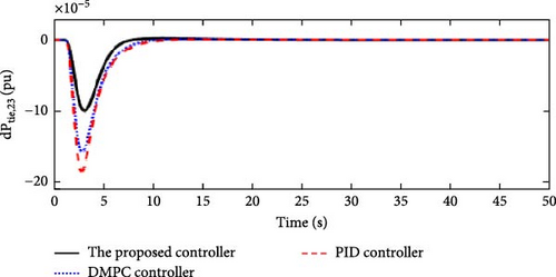
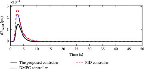
Controller	Δf₁(pu)			Δf₂(pu)			Δf₃(pu)			Δf₄(pu)
Controller	MO (pu)	MU (pu)	ST (s)	MO (pu)	MU (pu)	ST (s)	MO (pu)	MU (pu)	ST(s)	MO (pu)	MU (pu)	ST(s)
The proposed controller	0	3.3 × 10⁻⁴	9.4	0	1.67 × 10⁻⁴	10	0	1.6 × 10⁻⁴	11	0	1.5 × 10⁻⁴	10
DMPC controller	0	7 × 10⁻⁴	12	0	2.9 × 10⁻⁴	12	0	2.7 × 10⁻⁴	13	0	2.7 × 10⁻⁴	13
PID controller	1 × 10⁻⁴	8 × 10⁻⁴	14	0	3.3 × 10⁻⁴	14	0	3 × 10⁻⁴	15	0	3.1 × 10⁻⁴	15

Table 7. Results for Scenario (2) PDs.

Controller	ΔP_tie,12(pu)			ΔP_tie,23(pu)			ΔP_tie,34(pu)			ΔP_tie,41(pu)
Controller	MO (pu)	MU (pu)	ST (s)	MO (pu)	MU (pu)	ST (s)	MO (pu)	MU (pu)	ST (s)	MO (pu)	MU (pu)	ST (s)
The proposed controller	0	3.1 × 10⁻⁴	9.3	0	1 × 10⁻⁴	7	1.4 × 10⁻⁴	0	9	3.5 × 10⁻⁴	0	8
DMPC controller	0	5.84 × 10⁻⁴	11	0	1.7 × 10⁻⁴	9	2.4 × 10⁻⁴	0	10	6 × 10⁻⁴	0	10
PID controller	1 × 10⁻⁴	6.7 × 10⁻⁴	13	0	1.8 × 10⁻⁴	10	2.9 × 10⁻⁴	0	12	7.1 × 10⁻⁴	0	13

4.3. Scenario (3)

In this scenario, the time-varying wind speed is applied to the Area 1 of the multi-area power system as shown in Figure 21. Also, in this scenario, the effect of severe uncertainties in the parameters D and M (M = D = −20%) in each of the areas of the power system is considered. Figures 22, 23, 24, and 25 show the FDs of areas 1, 2, 3, and 4 using different control methods, respectively. Figures 26, 27, 28, and 29 show the PDs of the tie-line for areas 1–2, 2–3, 3–4, and 4–1 using different control methods, respectively. According to Figures 22–29, the proposed control method (H∞–DRL) has been able to reduce FDs, as well as PDs between tie-lines and has an effective performance against severe disturbances and severe uncertainties. The results for Scenario (3) are shown in Tables 8 and 9.

Table 8. Results for Scenario (3) FDs.

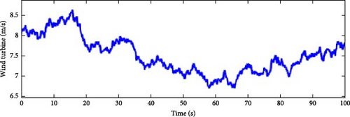
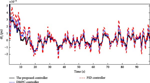
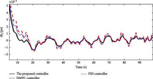
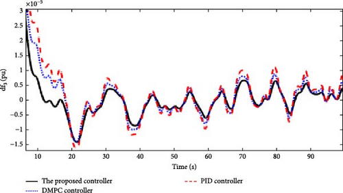
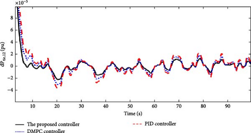
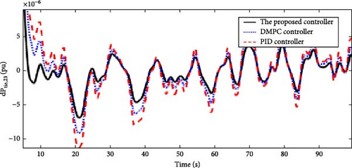
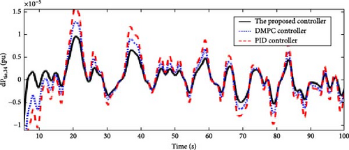
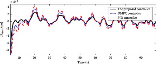
Controller	Δf₁(pu)	Δf₂(pu)	Δf₃(pu)	Δf₄(pu)
Controller	MFD (pu)	MFD (pu)	MFD (pu)	MFD (pu)
The proposed controller	5 × 10⁻⁵	5 × 10⁻⁵	4.5 × 10⁻⁵	4.4 × 10⁻⁵
DMPC controller	7 × 10⁻⁵	5 × 10⁻⁵	5.5 × 10⁻⁵	5.6 × 10⁻⁵
PID controller	8 × 10⁻⁵	6 × 10⁻⁵	6 × 10⁻⁵	6.4 × 10⁻⁵

Table 9. Results for Scenario (3) PDs.

Controller	ΔP_tie,12(pu)	ΔP_tie,23(pu)	ΔP_tie,34(pu)	ΔP_tie,41(pu)
Controller	MD (pu)	MD (pu)	MD (pu)	MD (pu)
The proposed controller	10 × 10⁻⁵	13 × 10⁻⁵	7 × 10⁻⁵	7.1 × 10⁻⁵
DMPC controller	11.5 × 10⁻⁵	17 × 10⁻⁵	8.5 × 10⁻⁵	11 × 10⁻⁵
PID controller	13 × 10⁻⁵	21 × 10⁻⁵	9.8	12 × 10⁻⁵

5. Conclusion

The frequency stability of the power system has been enhanced in this research by taking into account VIC and VDC for OWTs. However, the H∞ resilient controller based on DRL has been created in the structure of the LFC connected to the power system. It can adapt to uncertainties and is resistant to both disturbances and uncertainties related to the power system parameters. Several situations were taken into consideration in order to compare the suggested approach (H∞–DRL) with alternative control methods and the following outcomes were obtained:

•
Improvement of frequency deviations due to disturbances and uncertainties in the power system by 50%.
•
Improvement of communication line power deviations due to disturbances and uncertainties by 46%.

Nomenclature

α:: Coefficient of frequency deviation
T_ij:: The equivalent coefficient of tie-line i j
D_i:: The equivalent damping coefficient of i-th area
M_i:: The equivalent inertia coefficient of i-th area
T_r,i, T_t,i, T_g,i:: The equivalent inertia coefficient of i-th area
K_r,i:: Time constant of boiler, turbine and governor in i-th area
C_P:: Wind energy utilization coefficient
r:: Radius of the wind turbine blades
λ:: Wind energy utilization coefficient
P_m:: Mechanical power of WTG
P_e:: Output of the generator of WTG
v:: Wind speed
P_f:: Auxiliary frequency control command of WTG
ΔT:: Difference in torque between the electromagnetic power and the mechanical power
ω:: Rotor speed of WTG
T_e:: Time constant of generator of WTG
F:: Friction coefficient of the transmission system of WTG
K_c:: Maximum power tracking coefficient of WTG
ρ:: Density of air
ω_n:: Rated rotor speed
ω₀:: Initial rotor speed
Δf_i:: Frequency deviation of i-th area
ΔP_g,_i:: Output change of governor of thermal power plant in i-th area
ΔP_tie,i:: Tie-line power in i-th area
ΔP_L,i:: Load demand disturbance in i-th area
β:: Pitch angle
u_i:: Active power control signal of thermal power plant in i-th area
ΔXg,i:: Output change of boiler of thermal power plant in ith area
ΔP_r,i:: Output change of turbine of thermal power plant in i-th area
ACE_i:: area control error in i-th area
H_w:: Inertia coefficient of transmission system of WTG

Abbreviations

3DOF-PID:: Three degrees of freedom proportional–integral–derivative
DMPC:: Distributed model predictive control
DOSA:: Developed owl search algorithm
FDs:: Frequency deviations
FMPC:: Fuzzy model predictive control
FNN:: Feed-forward neural networks
FOPID:: Fractional-order proportional–integral–derivative
MO:: Maximum overshoot
MPC:: Model predictive control
MPPT:: Maximum power point tracking
MU:: maximum undershoot
PDs:: Power deviations
PI^λ (1+PDF):: Proportional–fractional integrator plus proportional–derivative with filter
RL:: Reinforcement learning
SMC:: Sliding mode controller
ST:: Settling time
TID:: Tilt-integral–derivative
TPP:: Thermal power plants
VDC:: Virtual damping control
WTs:: Wind turbines.

Conflicts of Interest

The authors declare no conflicts of interest.

Funding

This research was done without any financial support or funding.

Appendix

Table A1. Parameters related to the multi-area power system.

Parameter	Value	Parameter	Value
M_i	25	T_t,i	0.03
D_i	0.5	T_g,i	0.2
T₁₂	0.2	K_r,i	0.3
T₂₃	0.15	R	0.02
T₃₄	0.25	ω_n	1.091
T₄₁	0.21	λ_n	8.1
T_r	7	H_w	5.19
F	0.01	T_e	0.02
C_P	0.44	K_c	0.5787
K_P0	0.02	K_D0	46.6

Open Research

Data Availability Statement

The data are contained within the article.

References

1 Ali F., Shahidi A. E., Stewart R. A., Sanjari M. J., Hayward J. A., and Nicholson R., Co-Located Offshore Wind and Floating Solar Farms: A Systematic Quantitative Literature Review of Site Selection Criteria, Renewable Energy Focus. (2024) 50, https://doi.org/10.1016/j.ref.2024.100611, 100611.
10.1016/j.ref.2024.100611
Web of Science® Google Scholar
2 Shaheen M. A., Hasanien H. M., Mekhamer S. F., and Talaat H. E., Walrus Optimizer-Based Optimal Fractional Order PID Control for Performance Enhancement of Offshore Wind Farms, Scientific Reports. (2024) 14, no. 1, https://doi.org/10.1038/s41598-024-67581-x.
10.1038/s41598-024-67581-x
Web of Science® Google Scholar
3 Verma A. S., Jiang Z., Vedvik N. P., Gao Z., and Ren Z., Impact Assessment of a Wind Turbine Blade Root during an Offshore Mating Process, Engineering Structures. (2019) 180, 205–222, https://doi.org/10.1016/j.engstruct.2018.11.012, 2-s2.0-85056833822.
10.1016/j.engstruct.2018.11.012
Web of Science® Google Scholar
4 Lee N., Woo J., and Kim S., A Deep Reinforcement Learning Ensemble for Maintenance Scheduling in Offshore Wind Farms, Applied Energy. (2025) 377, https://doi.org/10.1016/j.apenergy.2024.124431, 124431.
10.1016/j.apenergy.2024.124431
Web of Science® Google Scholar
5 He R., Tian Z., Wang Y., Chen Y., and Zuo M. J., Predictive Maintenance for Offshore Wind Farms With Incomplete and Biased Prognostic Information, Ocean Engineering. (2025) 322, https://doi.org/10.1016/j.oceaneng.2025.120541, 120541.
10.1016/j.oceaneng.2025.120541
Web of Science® Google Scholar
6 Shid-Moosavi S., Di Cioccio F., and Haghi R., et al.Modeling and Experimentally-Driven Sensitivity Analysis of Wake-Induced Power Loss in Offshore Wind Farms: Insights From Block Island Wind Farm, Renewable Energy. (2025) 241, https://doi.org/10.1016/j.renene.2024.122126, 122126.
10.1016/j.renene.2024.122126
Web of Science® Google Scholar
7 Yang C., Jia J., and He K., et al.Comprehensive Analysis and Evaluation of the Operation and Maintenance of Offshore Wind Power Systems: A Survey, Energies. (2023) 16, no. 14, https://doi.org/10.3390/en16145562.
10.3390/en16145562
PubMed Web of Science® Google Scholar
8 Xiang W., Tu R., Han M., and Wen J., Hybrid AC/DC Collection and HVDC Transmission Topology for Large-Scale Offshore Wind Farms, CSEE Journal of Power and Energy Systems. (2025) doi: 10.17775/CSEEJPES.2024.05450.
Web of Science® Google Scholar
9 Rosencrans D., Lundquist J. K., Optis M., and Bodini N., The Effects of Wind Farm Wakes on Freezing Sea Spray in the Mid-Atlantic Offshore Wind Energy Areas, Wind Energy Science. (2025) 10, no. 1, 59–81, https://doi.org/10.5194/wes-10-59-2025.
10.5194/wes-10-59-2025
Web of Science® Google Scholar
10 Barnabei V. F., Ancora T., and Conti M., et al.A Multi-Objective Optimization Framework for Offshore Wind Farm Design in Deep Water Seas, Journal of Fluids Engineering. (2025) 147, no. 3, https://doi.org/10.1115/1.4067365.
10.1115/1.4067365
Web of Science® Google Scholar
11 Huang S., Wu Q., Bao W., Hatziargyriou N. D., Ding L., and Rong F., Hierarchical Optimal Control for Synthetic Inertial Response of Wind Farm Based on Alternating Direction Method of Multipliers, IEEE Transactions on Sustainable Energy. (2021) 12, no. 1, 25–35, https://doi.org/10.1109/TSTE.2019.2963549.
10.1109/TSTE.2019.2963549
Web of Science® Google Scholar
12 Skiparev V., Nosrati K., and Tepljakov A., et al.Virtual Inertia Control of Isolated Microgrids Using an NN-Based VFOPID Controller, IEEE Transactions on Sustainable Energy. (2023) 14, no. 3, 1558–1568, https://doi.org/10.1109/TSTE.2023.3237922.
10.1109/TSTE.2023.3237922
Web of Science® Google Scholar
13 Saxena A., Al Zaabi O., Al Jaafari K., Shankar R., Al Hosani K., and Muduli U. R., Optimal Virtual Inertia Control-Based Frequency Regulation of an Interconnected Microgrid With the Integration of Renewable Energy Sources, 2023 IEEE IAS Global Conference on Renewable Energy and Hydrogen Technologies (GlobConHT), March, 2023, Male, Maldives, IEEE, 1–6, https://doi.org/10.1109/GlobConHT56829.2023.10087581.
10.1109/GlobConHT56829.2023.10087581
Google Scholar
14 Bonfiglio A., Invernizzi M., Labella A., and Procopio R., Design and Implementation of a Variable Synthetic Inertia Controller for Wind Turbine Generators, IEEE Transactions on Power Systems. (2018) 34, no. 1, 754–764, https://doi.org/10.1109/TPWRS.2018.2865958, 2-s2.0-85059111391.
10.1109/TPWRS.2018.2865958
Google Scholar
15 Qi X., Madonski R., Huang C., and Ke Y., Tracking-Differentiator-Based Dynamic Virtual Inertial Control of Offshore Wind Power Plant for Frequency Regulation, International Journal of Electrical Power and Energy Systems. (2022) 141, https://doi.org/10.1016/j.ijepes.2022.108150, 108150.
10.1016/j.ijepes.2022.108150
Web of Science® Google Scholar
16 Margaris I. D., Papathanassiou S. A., Hatziargyriou N. D., Hansen A. D., and Sorensen P., Frequency Control in Autonomous Power Systems With High Wind Power Penetration, IEEE Transactions on Sustainable Energy. (2012) 3, no. 2, 189–199, https://doi.org/10.1109/TSTE.2011.2174660, 2-s2.0-84859024142.
10.1109/TSTE.2011.2174660
Web of Science® Google Scholar
17 Lee J., Jang G., Muljadi E., Blaabjerg F., Chen Z., and Kang Y. C., Stable Short-Term Frequency Support Using Adaptive Gains for a DFIG-Based Wind Power Plant, IEEE Transactions on Energy Conversion. (2016) 31, no. 3, 1068–1079, https://doi.org/10.1109/TEC.2016.2532366, 2-s2.0-84960540143.
10.1109/TEC.2016.2532366
Web of Science® Google Scholar
18 Lee J., Muljadi E., Srensen P., and Kang Y. C., Releasable Kinetic Energy-Based Inertial Control of a DFIG Wind Power Plant, IEEE Transactions on Sustainable Energy. (2016) 7, no. 1, 279–288, https://doi.org/10.1109/TSTE.2015.2493165, 2-s2.0-84958108865.
10.1109/TSTE.2015.2493165
Web of Science® Google Scholar
19 Amiri F., Eskandari M., and Moradi M. H., Improved Load Frequency Control in Power Systems Hosting Wind Turbines by an Augmented Fractional Order PID Controller Optimized by the Powerful Owl Search Algorithm, Algorithms. (2023) 16, no. 12, https://doi.org/10.3390/a16120539.
10.3390/a16120539
Web of Science® Google Scholar
20 Rouhanian A., Aliamooei-Lakeh H., Aliamooei-Lakeh S., and Toulabi M., Improved Load Frequency Control in Power Systems With High Penetration of Wind Farms Using Robust Fuzzy Controller, Electric Power Systems Research. (2023) 224, https://doi.org/10.1016/j.epsr.2023.109511, 109511.
10.1016/j.epsr.2023.109511
Web of Science® Google Scholar
21 Oshnoei S., Oshnoei A., Mosallanejad A., and Haghjoo F., Novel Load Frequency Control Scheme for an Interconnected Two-Area Power System including Wind Turbine Generation and Redox Flow Battery, International Journal of Electrical Power and Energy Systems. (2021) 130, https://doi.org/10.1016/j.ijepes.2021.107033, 107033.
10.1016/j.ijepes.2021.107033
Web of Science® Google Scholar
22 Wang H. and Li Z. S., Multi-Area Load Frequency Control in Power System Integrated With Wind Farms Using Fuzzy Generalized Predictive Control Method, IEEE Transactions on Reliability. (2022) 72, no. 2, 737–747, https://doi.org/10.1109/TR.2022.3177045.
10.1109/TR.2022.3177045
Web of Science® Google Scholar
23 Kamarposhti M. A., Shokouhandeh H., Alipur M., Colak I., Zare H., and Eguchi K., Optimal Designing of Fuzzy-PID Controller in the Load-Frequency Control Loop of Hydro-Thermal Power System Connected to Wind Farm by HVDC Lines, IEEE Access. (2022) 10, 63812–63822, https://doi.org/10.1109/ACCESS.2022.3183155.
10.1109/ACCESS.2022.3183155
Web of Science® Google Scholar
24 Khan I. A., Mokhlis H., and Mansor N. N., et al.Load Frequency Control in Power Systems With High Renewable Energy Penetration: A Strategy Employing PIλ (1+ PDF) Controller, Hybrid Energy Storage, and IPFC-FACTS, Alexandria Engineering Journal. (2024) 106, 337–366, https://doi.org/10.1016/j.aej.2024.06.087.
10.1016/j.aej.2024.06.087
Google Scholar
25 Guha D., Roy P. K., and Banerjee S., Equilibrium Optimizer-Tuned Cascade Fractional-Order 3DOF-PID Controller in Load Frequency Control of Power System Having Renewable Energy Resource Integrated, International Transactions on Electrical Energy Systems. (2021) 31, no. 1, https://doi.org/10.1002/2050-7038.12702, e12702.
10.1002/2050-7038.12702
Web of Science® Google Scholar
26 Abhayadev S. and Kumar P. R., Effect of DFIG Wind Turbines on LFC in a Sliding Mode Controlled Power System, 2021 6th International Conference for Convergence in Technology (I2CT), 02-04, April, 2021, Maharashtra, India, IEEE, 1–6, https://doi.org/10.1109/I2CT51068.2021.9418167.
10.1109/I2CT51068.2021.9418167
Google Scholar
27 Deng Z. and Xu C., Frequency Regulation of Power Systems With a Wind Farm by Sliding-Mode-Based Design, IEEE/CAA Journal of Automatica Sinica. (2022) 9, no. 11, 1980–1989, https://doi.org/10.1109/JAS.2022.105407.
10.1109/JAS.2022.105407
Web of Science® Google Scholar
28 Yang J., Sun X., Liao K., He Z., and Cai L., Model Predictive Control-Based Load Frequency Control for Power Systems With Wind-Turbine Generators, IET Renewable Power Generation. (2019) 13, no. 15, 2871–2879, https://doi.org/10.1049/iet-rpg.2018.6179.
10.1049/iet-rpg.2018.6179
Web of Science® Google Scholar
29 Liu X., Zhang Y., and Lee K. Y., Coordinated Distributed MPC for Load Frequency Control of Power System With Wind Farms, IEEE Transactions on Industrial Electronics. (2017) 64, no. 6, 5140–5150, https://doi.org/10.1109/TIE.2016.2642882, 2-s2.0-85028063025.
10.1109/TIE.2016.2642882
Web of Science® Google Scholar
30 Qi X., Lei L., and Yu C., et al.Adaptive Distributed MPC Based Load Frequency Control With Dynamic Virtual Inertia of Offshore Wind Farms, IET Control Theory and Applications. (2024) 18, no. 17, 2228–2238, https://doi.org/10.1049/cth2.12639.
10.1049/cth2.12639
Web of Science® Google Scholar
31 Cheng S., Li L., Liu C. Z., Wu X., Fang S. N., and Yong J. W., Robust LMI-Based H-Infinite Controller Integrating AFS and DYC of Autonomous Vehicles With Parametric Uncertainties, IEEE Transactions on Systems, Man, and Cybernetics: Systems. (2020) 51, no. 11, 6901–6910, https://doi.org/10.1109/TSMC.2020.2964282.
10.1109/TSMC.2020.2964282
Google Scholar
32 Mohanty S. R., Kishor N., and Ray P. K., Robust H-Infinite Loop Shaping Controller Based on Hybrid PSO and Harmonic Search for Frequency Regulation in Hybrid Distributed Generation System, International Journal of Electrical Power and Energy Systems. (2014) 60, 302–316, https://doi.org/10.1016/j.ijepes.2014.03.012, 2-s2.0-84899003962.
10.1016/j.ijepes.2014.03.012
Web of Science® Google Scholar
33 Chatavi M., Vu M. T., Mobayen S., and Fekih A., H∞ Robust LMI-Based Nonlinear State Feedback Controller of Uncertain Nonlinear Systems With External Disturbances, Mathematics. (2022) 10, no. 19, https://doi.org/10.3390/math10193518.
10.3390/math10193518
Web of Science® Google Scholar
34 Milani S., Topin N., Veloso M., and Fang F., Explainable Reinforcement Learning: A Survey and Comparative Review, ACM Computing Surveys. (2024) 56, no. 7, 1–36, https://doi.org/10.1145/3616864.
10.1145/3616864
Web of Science® Google Scholar
35 Albrecht S. V., Christianos F., and Schäfer L., Multi-Agent Reinforcement Learning: Foundations and Modern Approaches, 2024, MIT Press, Cambridge, Massachusetts.
Google Scholar
36 Meng Q., Hussain S., Luo F., Wang Z., and Jin X., An Online Reinforcement Learning-Based Energy Management Strategy for Microgrids With Centralized Control, IEEE Transactions on Industry Applications. (2025) 61, no. 1, 1501–1510, https://doi.org/10.1109/TIA.2024.3430264.
10.1109/TIA.2024.3430264
Web of Science® Google Scholar
37 Rolf B., Jackson I., Müller M., Lang S., Reggelin T., and Ivanov D., A Review on Reinforcement Learning Algorithms and Applications in Supply Chain Management, International Journal of Production Research. (2023) 61, no. 20, 7151–7179, https://doi.org/10.1080/00207543.2022.2140221.
10.1080/00207543.2022.2140221
Web of Science® Google Scholar

All articles

Designing a New Control Method to Improve the LFC Performance of the Multi-Area Power System Considering the Effect of Offshore Wind Farms on Frequency Control

Abstract

1. Introduction

2. The Dynamic Model of Power System Considering the Effect of OWFs in Frequency Control