Mathematical Model of Human Papillomavirus (HPV) Dynamics With Double-Dose Vaccination and Its Impact on Cervical Cancer
Abstract
We develop a deterministic mathematical model to investigate the transmission dynamics of human papillomavirus (HPV) and its impact on cervical cancer. The model divides the population into six classes: susceptible individuals (S(t)), first vaccinated individuals (V(t)), permanently immunized individuals (P(t)), HPV-infected individuals (IHPV(t)), HPV-infected individuals with cervical cancer (C(t)), and recovered individuals (R(t)). The study includes analyzing the stability of the disease-free and endemic equilibriums. The analysis reveals that the disease-free equilibrium is locally asymptotically stable when the average number of secondary HPV-infectious individuals (R0) is less than one and unstable when it is greater than one. A stable local endemic equilibrium occurs when the average number of secondary HPV-infectious individuals exceeds one, indicating the persistence of the disease in the community. The value of R0 is derived using the next-generation matrix approach, revealing that HPV-infected individuals persist in the community. MATLAB 2015a is used to represent the simulation findings visually. The numerical simulation suggests that increasing vaccination coverage and the recovery rate helps to reduce HPV-infected individuals while reducing the contact rate can effectively control disease transmission.
1. Introduction
Human papillomavirus (HPV) is small DNA tumor viruses and is estimated to be the most common sexually transmitted viruses in humans [1]. Most HPV-infected individuals can spread the virus without showing symptoms. Out of the 100 types of HPV, 40 are high risk and can infect genital areas, the mouth, and throat. Persistent infection with HPV-16 and HPV-18 is responsible for about 70% of cervical cancers, posing a significant risk to women’s health worldwide [2]. Women with HIV are at an increased risk of developing cervical cancer, and several risk factors for the disease are linked to exposure to HPV infection, multiple sexual partners, a weakened immune system, and smoking [3–7].
Regional disparities in cervical cancer burden stem from unequal access to vaccination, screening, and treatment services, compounded by health, social, and economic factors. Early detection and effective techniques are crucial for successful treatment [8]. Pap smear screening is widely used for early detection, while developed countries offer advanced screening methods for predicting precancerous lesions [9, 10]. Treatment options include hysterectomy, radiation, and chemotherapy. Despite its severity, cervical cancer can be overcome with better health precautions [11].
The effectiveness of cervical cancer detection techniques is limited due to a lack of resources and trained health workers in developing countries. According to a 2024 report from the World Health Organization (WHO), there were approximately 660,000 new cases of cervical cancer in 2022, resulting in 350,000 deaths. 94% of these deaths occurred in sub-Saharan Africa (SSA), Central America, and South-East Asia. Research conducted in developing countries like Ethiopia reveals a growing incidence and prevalence of cervical cancer over time. For instance, the WHO reported that Ethiopia has a population of 36.9 million women aged 15 years and older who are at risk of developing cervical cancer [12]. According to this finding, the International Agency for Research on Cancer estimates that the number of new cervical cancer cases in Ethiopia will increase from 7500 in 2020 to 15,300 in 2040. The mortality rate is also projected to rise from 5340 in 2020 to 11,000 in 2040 annually. Despite limited high-quality cancer registries and reliable data, cervical cancer is increasingly contributing to morbidity and mortality among Ethiopian women due to the country’s inability to sustain effective cervical cancer prevention programs [13].
Understanding disease dynamics is essential for improving management strategies. Mathematical models of infectious diseases provide public health authorities with detailed insights into disease dynamics, helping them make informed decisions and policies. Deterministic models based on classical derivatives are commonly used to study disease transmission dynamics and predict future disease trends. While there have been limited mathematical studies on cervical cancer, some models have been developed to investigate HPV transmission dynamics and potential preventive measures. The authors in [14] developed the SI model for HPV transmission and cervical cancer infection in the United States, while the authors in [15] introduced the SIR model for HPV dynamics as a mathematical model for HPV in Ghana. The authors in [16] proposed the SIS epidemic model for HPV in males and females, and the authors in [17] formulated a two-sex compartmental model of HPV infection with time-dependent controls.
The research conducted by Al-Arydah [18] involved the development of an age-structured model for HPV vaccination programs. They considered the age and gender distribution of the population and looked at the effectiveness of vaccinating females early and providing catchup vaccinations for Types 6 and 11. The findings suggested that infection could potentially be eradicated in male and female populations over 30 years of age. The study also discussed the most cost-effective approach to implementing the catchup vaccine. The studies by Madhu [19] and Al-Arydah [20] developed mathematical models to assess the effectiveness of childhood and catchup vaccines in controlling HPV disease. Al-Arydah’s research suggested that adult-only vaccines represent a cost-effective strategy, with a focus on the impact of health education on vaccine uptake. The study also introduced an optimization problem to determine the best approach for maximizing vaccine uptake and controlling HPV at the lowest cost. Similarly, Madhu’s study highlighted the effectiveness of reducing the number of partners among youths and adults in decreasing HPV cases. Both studies emphasized the importance of health education in controlling HPV and optimizing vaccine coverage.
As far as we know, no mathematical modeling study has been conducted on the dynamics of this disease by considering double-dose vaccination. Therefore, we have utilized a mathematical model of HPV transmission dynamics with double-dose vaccination. This paper is structured as follows. Section 2 outlines the model formulation, Section 3 covers the model analysis, Section 4 discusses the numerical simulation of the model, and Section 5 presents the conclusions of this study.
2. Model Formulation
| Parameters | Description |
|---|---|
| π | Recruitment rate |
| β | Transmission rate |
| α | First-dose vaccination rate |
| δ | Loss of the first vaccination rate (attrition rate) |
| θ | The rate at which the first vaccination-vaccinated individual joins the permanently immunized compartment |
| ω | Rate at which people lose immunity and become susceptible |
| μ | Natural death rate |
| ϑ | Progression rate from HPV infection to cervical cancer |
| γ | Recovery rate of HPV-infected individuals |
| φ | The mortality rate for individuals due to cervical cancer disease. |
- 1.
The susceptible population consists of all women whose ages are above fifteen.
- 2.
The population consists of a homogeneous mixture of individuals.
- 3.
First-dose vaccinated person may become susceptible again due to waning immunity.
- 4.
Recovered individuals are assumed to move back to the susceptible class.
- 5.
Individuals who have received the second dose will be fully protected from HPV.
- 6.
All parameters are positive.
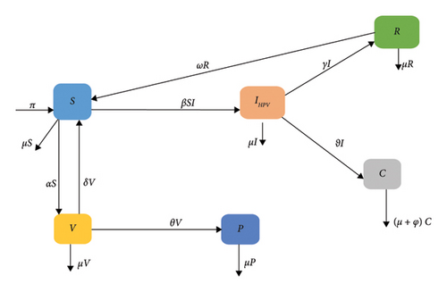
3. Model Analysis
In this section, we examined the qualitative behavior of the model, including positivity, boundedness, equilibrium points, the basic reproductive number, and sensitivity analysis.
3.1. Positivity and Boundedness of the Solutions
Since all components of the given model system consider a human population, it is necessary to demonstrate that all state variables S(t), V(t), IHPV(t), P(t), R(t), and C(t) are positive for all t > 0.
Theorem 1. Each solution of S(t), V(t), IHPV(t), P(t), R(t), and C(t) of model (2) with the non-negative initial condition is non-negative for all t t > 0.
Proof 1. Let us verify the positivity of each state variable of the model from the system of equation (2). From the second equation of system of equation (2), we have
Without considering the positive part of equation (3), we get
By applying the method of separation of variables to equation (4) and integrating both sides with respect to t, we obtain S(t) ≥ S(0)exp(∫−(α + μ + βIHPV))dt ≥ 0.
From the second equation of system of equation (2), we have
When applying the variable separation method to equation (5) and integrating both sides with respect to t, we obtain V(t) ≥ V(0)exp(−(μ + δ + θ)t). In a similar fashion, the solution for the other state variables is calculated using the same method we used for S(t) and V(t), resulting in P(t) ≥ P(0)exp(−μt), IHPV(t) ≥ IHPV(0)exp(−βS − (μ + γ + ϑ))dt, and C(t) ≥ C(0)exp(−(μ + φ)t), R(t) ≥ R(0)exp(−(ω + μ)t). Thus, all state variables of the system are positive for t > 0. As the solutions for all state variables are exponential functions of t and the functional value of the exponential function is always positive, the solution for all state variables of the system is positive for t > 0.
Theorem 2. The feasible solution set {S, V, P, IHPV, C, R} of the model equation (2) with the given initial condition remains bound in the region .
Proof 2. To prove Theorem (2), let us differentiate both sides of equation (1) with respect to t that gives
Using system equation (2) and evaluating at equation (6) give us
In equation (7), if there is no death due to cervical cancer (φ ≠ 0), and the state variable of the system of equation (2) is positive for all t ≥ 0. As a result, equation (6) becomes
In solving inequality in equation (8), we used the method of separation of variables and integrate both sides with respect to t as follows:
Here, from equation (9), as t⟶∞, then N(t) is asymptotically bounded within the range 0 ≤ N(t) ≤ π/μ. This concludes the proof.
3.2. Disease-Free Equilibrium Point
3.3. Endemic Equilibrium Point
3.4. Basic Reproductive Number of the Model
The roots of the characteristic polynomial equation of (36) are λ1 = 0 and λ2 = βπ(μ + θ + δ)/((μ + θ)(α + μ) + μδ)(μ + γ + ϑ). According to the principle of the next generation matrix, the largest solution of characteristic polynomial equation (eigenvalue of the Jacobian matrix) is the basic reproductive number. Therefore, R0 = (βπ(μ + θ + δ))/(((μ + θ)(α + μ) + μδ)(μ + γ + ϑ)).
3.5. Local Stability of the Disease-Free Equilibrium Point
In order to determine the stability of the disease-free equilibrium point in the system of equation (2), we need to compute the characteristic equation of the Jacobian matrix . This can be done by examining the eigenvalues of the corresponding Jacobian matrix, which depend on the model parameters.
Theorem 3. The disease-free equilibrium point of the system of equation (2) is locally asymptotically stable if R0 < 1 and unstable if R0 > 1.
Proof 3. To prove this theorem, we first construct the Jacobian matrix of the system of equation (1). To simplify this, let us represent f1 = π + δV + ωR − (α + μ + βIHPV)S, f2 = αS − (μ + δ + θ)V, f3 = θV − μP, f4 = βIHPVS − (μ + γ + ϑ)IHPV, f5 = ϑIHPV − (μ + φ)C, and f6 = γIHPV − (ω + μ)R. Then,
The Jacobian matrix at the disease-free equilibrium point becomes
Let X1 = α + μ, X2 = μ + δ + θ, X3 = βS0 − (μ + γ + ϑ), X4 = μ + φ, and X5 = μ + ω. Then, the characteristic polynomial equation of is computed by taking the determinant of , where I represents the identity matrix.
Next, we have to compute the corresponding eigenvalues of which is the same as the roots of p(λ).
Since the parameter’s values are assumed positive, then the first three roots of the characteristic equation (41), denoted as λ1 = −μ, λ2 = −(μ + φ ), and λ4 = −(μ + ω), have negative values. A study by Mahardika and Sumanto [21] noted that, as per the Routh–Hurwitz stability condition, the equation system is stable only if all roots of the characteristic equation are negative. For a quadratic function to be stable, both coefficients must be greater than zero. Then,
- i.
X1 + X2 > 0⟹α + μ + μ + δ + θ > 0
- ii.
X1X2 − αδ⟹(α + μ)(μ + δ + θ) − αδ, ⟹α(μ + δ + θ) + μ(μ + δ + θ) − αδ, ⟹α(μ + θ) + μ(μ + δ + θ) > 0 (because all values of parameters are assumed positive)
- iii.
The system equation (2) is stable when the values of λ3 are negative. This implies that S0 − (μ + γ + ϑ) < 0⟹βS0 < (μ + γ + ϑ), (βS0/(μ + γ + ϑ)) < 1⟹βπ(μ + θ + δ)/((μ + θ)(α + μ) + μδ)(μ + γ + ϑ) < 1.
Since R0 = βπ(μ + θ + δ)/((μ + θ)(α + μ) + μδ)(μ + γ + ϑ), then the disease-free equilibrium point of the system of equation (2) is locally asymptotically stable, if R0 < 1.
3.6. Global Stability of the Disease-Free Equilibrium Point
To prove this theorem, we will construct a Lyapunov function, focusing on the infected classes of equation system (2).
Theorem 4. The disease-free equilibrium point of system of equation (2) is globally asymptotically stable if R0 < 1.
Proof 4. To prove this theorem, we constructed a Lyapunov function, focusing on the infected classes of system of equation (2) as follows:
Next, substituting (dIHPV/dt) and (dC/dt) from the system of equation (2) into equation (43) gives
Let us take u2 = (βπ(μ + θ + δ)/(μ + θ)(α + μ) + μδ − (μ + γ + ϑ)/(μ + γ + ϑ))u1. Then, at the disease-free equilibrium point, equation (44) becomes
According to the Lyapunov principle, the disease-free equilibrium point of the system of equation is satisfied if (dL/dt) < 0. From equation (45), (dL/dt) < 0 if R0 < 1, which reveal that the disease-free equilibrium point of the system of equation (2) is globally asymptotically stable if R0 < 1. Hence, the theorem is verified.
3.7. Local Stability of the Endemic Equilibrium Point of the Model
Before we verify the stability of the endemic equilibrium point, we need to check if this point exists. If it does, we have to determine if it is unique.
Theorem 5. The model has a unique endemic equilibrium point if R0 > 1.
Proof 5. At this point, both IHPV and C are greater than zero. This implies that
- i.
IHPV > ⟹(((μ + δ + θ)βπ − (μ + γ + ϑ)((μ + θ)(α + μ) + μδ))(ω + μ))/(μ + δ + θ)((μ + ϑ)(ω + μ) + γμ)β > 0, ⟹((μ + γ + ϑ)((μ + θ)(α + μ) + μδ)(ω + μ)/(μ + δ + θ)((μ + ϑ)(ω + μ) + γμ)β)((μ + δ + θ)βπ/(μ + γ + ϑ)((μ + θ)(α + μ) + μδ) − 1) > 0, ⟹((μ + γ + ϑ)((μ + θ)(α + μ) + μδ)(ω + μ)/(μ + δ + θ)((μ + ϑ)(ω + μ) + γμ)β)(R0 − 1) > 0.
- ii.
C > 0⟹((μ + δ + θ)βπ − (μ + γ + ϑ)((μ + θ)(α + μ) + μδ))ϑ(ω + μ)/(μ + δ + θ)((μ + ϑ)(ω + μ) + γμ)(μ + φ)β > 0, ⟹((μ + γ + ϑ)((μ + θ)(α + μ) + μδ)(ω + μ)ϑ/(μ + δ + θ)((μ + ϑ)(ω + μ) + γμ)β)((μ + δ + θ)βπ/(μ + γ + ϑ)((μ + θ)(α + μ) + μδ)1), ⟹((μ + γ + ϑ)((μ + θ)(α + μ) + μδ)(ω + μ)ϑ/(μ + δ + θ)((μ + ϑ)(ω + μ) + γμ)β)(R0 − 1).
The inequality in i and ii holds if R0 > 1. This indicates that based on the developed model, HPV disease persists in the community (the endemic equilibrium point is existed) when R0 > 1.
Theorem 6. An endemic equilibrium point of system of equation (2) is locally asymptotically stable when R0 > 1.
Proof 6. In order to prove this theorem, we constructed the Jacobian matrix J of the system of equation (2) using equation (37) at the endemic equilibrium point. To compute the characteristic equation from the developed Jacobian matrix, let us represent Y1 = (α + μ + βIHPV), Y2 = (μ + δ + θ), Y3 = (μ + φ), Y4 = (μ + ω), and Y5 = βIHPV. Then,
Again, to write equation (46) in a simplified form, let us use b1 = Y1 + Y2 + Y4, , b3 = ((Y2 + Y4)βS∗ − ωγ)Y5 + (Y1Y2 − δα)Y4, and b4 = (βS∗Y4 − ωγ)Y2Y5. This simplification leads to
Next, we have to find the roots of characteristic equation (47) which is the same as eigenvalues of JEEp from p(λ) = 0.
The first two roots’ characteristic of equation (47) is negative, that is, λ1 = −μ and λ2 = −Y3 = (μ + φ). To determine the stability condition of the system model at the endemic equilibrium point, we applied the Routh–Hurwitz stability condition on equation (48) as follows:
- i.
b1 > 0⟹Y1 + Y2 + Y4 > 0⟹α + 3μ + δ + θ + ω + βIHPV > 0, α + 3μ + δ + θ + ω + β(((μ + δ + θ)βπ − (μ + γ + ϑ)((μ + θ)(α + μ) + μδ))(ω + μ)/(μ + δ + θ)((μ + ϑ)(ω + μ) + γμ)β) > 0, α + 3μ + δ + θ + ω + ((μ + γ + ϑ)((μ + θ)(α + μ) + μδ)(ω + μ)/(μ + δ + θ)((μ + ϑ)(ω + μ) + γμ))((μ + δ + θ)βπ/(μ + γ + ϑ)((μ + θ)(α + μ) + μδ) − 1) > 0, ⟹3μ + α + δ + θ + ω + ((μ + γ + ϑ)((μ + θ)(α + μ) + μδ)(ω + μ)/(μ + δ + θ)((μ + ϑ)(ω + μ) + γμ))(R0 − 1) > 0.
- ii.
.
- iii.
b3 > 0⟹((Y2 + Y4)βS∗ − ωγ)Y5 + (Y1Y2 − δα)Y4 = ((2μ + δ + θ)(μ + γ + ϑ) + ω(μ + ϑ) + (μ + δ + θ)(μ + ω))βIHPV + ((α + μ)(μ + θ) + μδ)(μ + ω) > 0 = ((α + μ)(μ + θ) + μδ)(μ + ω) + ((2μ + δ + θ)(μ + γ + ϑ) + ω(μ + ϑ) + (μ + δ + θ)(μ + ω))((μ + γ + ϑ)((μ + θ)(α + μ) + μδ)(ω + μ)/(μ + δ + θ)((μ + ϑ)(ω + μ) + γμ))(R0 − 1) > 0
- iv.
b4 > 0⟹(βS∗Y4 − ωγ)Y2Y5 > 0. This holds if (βS∗Y4 − ωγ) > 0 and Y2Y5 > 0 or (βS∗Y4 − ωγ) < 0 and Y2Y5 < 0
- a.
βS∗Y4 − ωγ > 0⟹β((μ + γ + ϑ)/β)(μ + ω) − ωγ = (μ + ϑ)(μ + ω) + γμ > 0.
- b.
Y2Y5 > 0⟹(((μ + δ + θ)βπ − (μ + γ + ϑ)((μ + θ)(α + μ) + μδ))(ω + μ)/((μ + ϑ)(ω + μ) + γμ)) > 0, ((μ + γ + ϑ)((μ + θ)(α + μ) + μδ)(ω + μ)/((μ + ϑ)(ω + μ) + γμ))((μ + δ + θ)βπ)/((μ + γ + ϑ)((μ + θ)(α + μ) + μδ) − 1) > 0, ((μ + γ + ϑ)((μ + θ)(α + μ) + μδ)(ω + μ)/((μ + ϑ)(ω + μ) + γμ))(R0 − 1) > 0.
- a.
- v.
b1b2 − b3 > 0⟹(Y1βS∗ + ωγ)Y5 + (Y4Y1 + Y2Y4)(Y1 + Y2 + Y4) + (Y2Y1 − δα)(Y1 + Y2 + 2Y4) > 0, = (α + 3μ + δ + θ + ω + ((μ + γ + ϑ)((μ + θ)(α + μ) + μδ)(ω + μ)/(μ + δ + θ)((μ + ϑ)(ω + μ) + γμ))(R0 − 1)) + ((μ + θ)(α + μ + ((μ + γ + ϑ)((μ + θ)(α + μ) + μδ)(ω + μ)/(μ + δ + θ)((μ + ϑ)(ω + μ) + γμ))(R0 − 1)) + δ(μ + βIHPV))(α + δ + θ + 5μ + ((μ + γ + ϑ)((μ + θ)(α + μ) + μδ)(ω + μ)/(μ + δ + θ)((μ + ϑ)(ω + μ) + γμ))(R0 − 1) + 2ω) > 0.
- vi.
- vii.
.
Based on conditions i − vii, an endemic equilibrium of the system of equation (2) is locally asymptotically stable if R0 > 1, assuming all parameters are positive.
3.8. Global Stability of the Endemic Equilibrium Point
Theorem 7. The unique endemic equilibrium point of the system of equation (2) is globally asymptotically stable if R0 > 1.
Proof 7. We can use the Lyapunov function method to show that the system’s unique endemic equilibrium point is globally asymptotically stable when R0 > 1. Let us consider the following Lyapunov function , which is constructed technically:
Next, we need to differentiate both sides of equation (49) with respect to t, which can be expressed as follows:
At the endemic equilibrium point, equation (50) becomes
In order to write equation (51) in a simplify form, let us represent
Then, equation (52) becomes
Based on the study established by Gao et al. [22] and Saha and Ghosh [23], from equation (53), when a1 ≤ a2, indicating global asymptotic stability. This means that does not increase along the system’s trajectories, indicating the existence of global asymptotic stability and ensuring convergence to the endemic equilibrium point regardless of initial conditions.
3.9. Sensitivity Analysis and Its Interpretation
- 1.
For xi = π, PπR0 = (∂R0/∂π)∗π/R0 = β(μ + θ + δ)/((μ + θ)(α + μ) + μδ)(μ + γ + ϑ)∗π((μ + θ)(α + μ) + μδ)(μ + γ + ϑ)/πβ(μ + θ + δ) = 1.
- 2.
For xi = β, PβR0 = (∂R0/∂β)∗β/R0 = π(μ + θ + δ)/((μ + θ)(α + μ) + μδ)(μ + γ + ϑ)∗β((μ + θ)(α + μ) + μδ)(μ + γ + ϑ)/βπ(μ + θ + δ) = 1.
- 3.
For xi = δ, PδR0 = (∂R0/∂δ)∗δ/R0 = (βπα(μ + θ)(α + μ)(μ + γ + ϑ)/(((μ + θ)(α + μ) + μδ)(μ + γ + ϑ))2)∗δ((μ + θ)(α + μ) + μδ)(μ + γ + ϑ)/βπ(μ + θ + δ) = αδ(μ + θ)(α + μ)/((μ + θ)(α + μ) + μδ)(μ + θ + δ).
- 4.
For xi = α, PαR0 = (∂R0/∂α)∗α/R0 = −(βπ(μ + θ + δ)(μ + θ)(μ + γ + ϑ)/(((μ + θ)(α + μ) + μδ)(μ + γ + ϑ))2)∗α((μ + θ)(α + μ) + μδ)(μ + γ + ϑ)/βπ(μ + θ + δ) = −((μ + θ)α/((μ + θ)(α + μ) + μδ)).
- 5.
For xi = θ, PθR0 = (∂R0/∂θ)∗θ/R0 = (βπ((μ + θ)(α + μ) + μδ)(μ + γ + ϑ) − βπ(μ + θ + δ)(α + μ)(μ + γ + ϑ)/(((μ + θ)(α + μ) + μδ)(μ + γ + ϑ))2)∗θ((μ + θ)(α + μ) + μδ)(μ + γ + ϑ)/βπ(μ + θ + δ) = −αδθ/((μ + θ)(α + μ) + μδ)(μ + θ + δ).
- 6.
For xi = γ, PγR0 = (∂R0/∂γ)∗γ/R0 = −(βπ(μ + θ + δ)((μ + θ)(α + μ) + μδ)/(((μ + θ)(α + μ) + μδ)(μ + γ + ϑ))2)∗γ((μ + θ)(α + μ) + μδ)(μ + γ + ϑ)/βπ(μ + θ + δ) = −γ/μ + γ + ϑ.
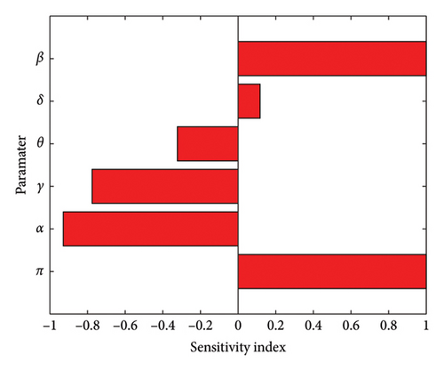
Based on the data presented in Table 2 and Figure 2, the HPV transmission rate (β) is the most crucial parameter, followed by the first-dose vaccination rate (α), recovery rate of HPV-infected individuals (γ), second-dose vaccination rate (θ), and the lowest attrition rate (δ). For example, PβR0 = 1 indicates that increasing the transmission rate by 10% leads to a 10% increase in the number of secondary HPV infections. On the other hand, for PαR0 = −0.9290, if we increase the first-dose vaccination rate by 10%, it results in a 9.29% decrease in secondary infections. Similarly, in PγR0 = −0.7758, if we increase the recovery rate of HPV-infected people by 10%, it leads to a 7.758% decrease in secondary infections, and for PθR0 = −0.3223, 10% increase in the second-dose vaccination rate results in a 3.223% decrease in secondary infections. Furthermore, for PδR0 = 0.1166, a 10% increase in the attrition rate leads to a 1.166% increase in secondary infections. Therefore, in order to mitigate the spread of HPV within the community, stakeholders and policymakers should aim to increase the first vaccination rate, recovery rate, and second-dose vaccination rate while simultaneously reducing the transmission rate and attrition rate.
| Parameters | Description | Sensitivity indicators |
|---|---|---|
| π | Recruitment rate | 1 |
| β | Transmission rate | 1 |
| α | First-dose vaccination-vaccinated rate | −0.9290 |
| γ | Recovery rate of HPV-infected people | −0.7758 |
| θ | Second-dose vaccination rate | −0.3223 |
| δ | Loss of the first vaccination rate (attrition rate) | 0.1166 |
| Parameters | Description | Values | Source |
|---|---|---|---|
| π | Recruitment rate | 0.588802 | Assumed |
| β | Transmission rate | 0.556 | Rajan et al. [26] |
| α | First-dose vaccination rate | 0.87 | Omame et al. [27] |
| δ | Loss of the first vaccination rate (attrition rate) | 0.1 | Malik et al. [28] |
| θ | The rate at which the first vaccination-vaccinated individual joins the permanently immunized compartment | 0.125 | Assumed |
| ω | The rate at which people lose immunity and become susceptible to HPV | 0.3 | Assumed |
| μ | Natural death rate | 0.0162 | Omame et al. [27] |
| ϑ | Progression rate from HPV infection to cervical cancer | 0.05714 | Rajan et al. [26] |
| γ | Recovery rate of HPV-infected individuals | 0.15 | Assumed |
| φ | The mortality rate for individuals due to cervical cancer disease | 0.01 | Malik et al. [28] |
4. Numerical Simulations
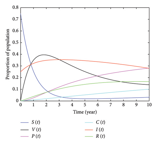
This section outlines the qualitative behavior of the model we developed, demonstrated through numerical simulation. Our focus is on analyzing the impact of double-dose vaccination on controlling HPV and reducing the number of individuals with cervical cancer. To conduct these simulations, we used MATLAB R2015a computer software to display the graph of the system of equation (2) and used parameter values from relevant published studies. We also tested the average value of secondary infectious people caused by a single infectious individual (R0), which was found to be R0 = 2.7893. Since the obtained value is greater than one, it verifies the existence of the endemic equilibrium point of the system equation (2), confirming the assertion made in Theorem 6, which indicates that the disease persists in the community and that the endemic equilibrium point exists and is unique. Figure 3, plotted using the parameter values provided in Table 3, represents the graphs of S(t), V(t), P(t), IHPV(t), C(t), and R(t). Figure 3 illustrates that, over time, the number of susceptible populations approaches zero due to the implementation of preventative measures, such as increased double vaccination. Conversely, the populations in the recovery and protected classes will increase. In this figure, it is shown that the maximum percentage of HPV-infected individuals is 35.43%, which occurred in the third year. To examine the impact of incorporating a double dose of vaccination, we tested its effect on the number of HPV-infected individuals. In the fifth year, 34.54% of the individuals were infected with HPV, and in the 10th year, this number decreased to 27.98%. We conducted a study on the impact of vaccination on individuals who are at risk of HPV infection. Over the first 2 years, as the number of people vaccinated increased, the number of susceptible individuals rapidly decreased. For instance, after 1 year, when 34.92% of the population was vaccinated, the percentage of susceptible individuals decreased to 25.46%. After 2 years, with 39.57% vaccinated, the percentage of susceptible individuals decreased to 10.6%. In the third year, with 35.43% vaccinated, the number of vulnerable individuals rapidly decreased to 3.792%. However, when the number of vaccinated individuals decreased, the number of vulnerable individuals increased. For example, in the 10th year, with only 13.9% of the population vaccinated, 3.809% of the population became vulnerable to HPV. In addition, we examined the impact of receiving the second dose of the vaccine on HPV-infected individuals. In the fifth year, 18.99% were protected from the virus, while 34.54% were infected. After 2 years, 23.84% were protected, while 32.49% were infected. This demonstrates that as people receive the double dose of the vaccine, the percentage of individuals infected with HPV decreases.
4.1. The Impact of the Contact Rate on HPV and Cervical Cancer in Infected Individuals
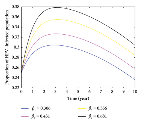
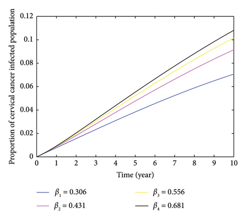
Here, we investigate the impact of contact rate on HPV-infected populations. From Figure 4, we can understand that increasing the contact rate leads to a significant rise in the number of HPV-infected individuals. This happens when susceptible individuals come into contact with HPV-infected individuals. Moreover, the figure demonstrates that an increase in the contact rate results in a higher number of HPV-infected individuals, which can lead to an expansion of cervical cancer cases. We computed the average number of secondary HPV-infected individuals caused by a single HPV infectious individual by varying the contact rate and obtained the respective values which is depicted as follows: when the contact rate increases from β3 = 0.556 to β4 = 0.75, the number of secondary HPV-infected individuals rises from 2.7893 to 3.7626. Conversely, when the contact rate decreases from β3 = 0.556 to β2 = 0.45, the average number of secondary HPV-infected individuals decreases from 2.2576 to 1.5828. This indicates that decreasing the rate of contact between HPV-infected and HPV-susceptible individuals helps reduce and potentially eradicate the spread of HPV. In Figure 4, the peak of HPV-infected individual was observed in the third year, resulting 37.87% when the contact rate β4 = 0.681. Furthermore, Figure 5 demonstrates that as the contact rate increases, the number of cervical cancer cases also increases, which is caused by an indirect increment of HPV-infected individuals. Therefore, based on the varied contact rates and the respective average number of secondary infectious, it is important to take measures to control the spread of HPV within the community by minimizing the rate of contact.
4.2. The Impact of the Waning Effectiveness of the First Dose of Vaccination on Individuals Infected With HPV
In Figure 6, it is evident that the number of HPV-infected individuals is on the rise due to a decrease in the number of people receiving their initial HPV vaccination. This trend may be attributed to many individuals not obtaining the crucial second vaccination dose, which is necessary for long-term immunity against HPV. To investigate this hypothesis, we calculated the basic reproductive number by adjusting the rate at which the effectiveness of the first vaccination diminishes. Our findings revealed that when the rate of waning effectiveness of the first vaccination dose (δ) changed from 0.05 to 0.125, the average number of secondary HPV-infected individuals increased from 2.2253 to 3.0686. This indicates a higher average number of secondary HPV-infected individuals when the attrition rate is increasing. It is evident that to control the spread of HPV and reduce cervical cancer in the community, individuals must receive the second vaccination dose before the effectiveness of the first vaccine wanes.

4.3. Impact of the Rate at Which Individuals Infected With HPV Progress to Developing Cervical Cancer
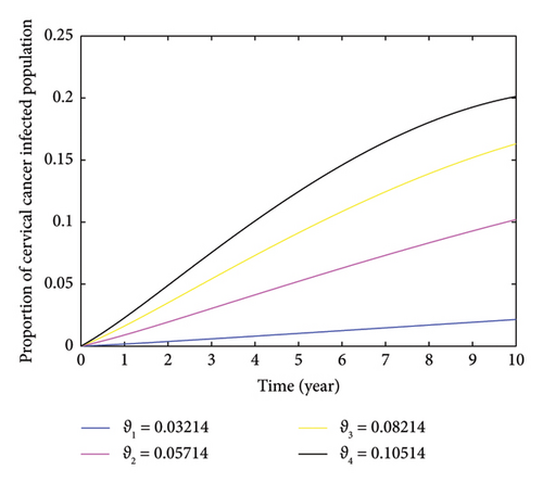
The impact of the rate of cervical cancer development in individuals infected with HPV is illustrated in Figure 7. The figure shows that an increase in the rate of cervical cancer development results in a higher number of individuals in the community being infected with cervical cancer, assuming all other factors remain constant. This increase is linked to the absence of treatment for individuals infected with HPV. Without proper treatment, the virus can persist in infected individuals for extended periods and eventually lead to the development of cervical cancer. This relationship is explored by varying the value of ϑ from 0.03214 to 0.10514. When these values are 0.03214, 0.05714, 0.08214, and 0.10514, the proportion of cervical cancer-infectious individuals within the 10 years also varied to 2.151%, 10.2%, 16.31%, and 20.12%, respectively.
4.4. The Influence of the Vaccinations Rate on the Population Infected With HPV
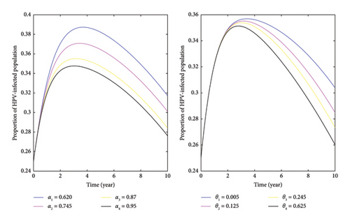
Based on the data presented in Figure 8, it is evident that as the rates of first- and second-dose vaccinations increase, the number of HPV-infected individuals decreases. This indicates that vaccinating individuals before they are exposed to the virus, especially females who receive both doses of the vaccine, can aid in controlling HPV and cervical cancer. Our analysis involved simulating different vaccination rates while keeping other factors constant. The results showed that higher vaccination rates led to a decrease in the average number of secondary HPV-infected individuals. The left-hand side of the figure demonstrates that the peak proportion of HPV-infected individuals, at 38.73%, occurred when the rate of first vaccination α1 = 0.620 occurred around the fourth year. However, increasing the first vaccination rate to α3 = 0.87 corresponded to a decrease in the proportion of HPV-infected individuals to 35.51%. Meanwhile, after the fourth year, the proportion of HPV-infectious individuals steadily decreased. Furthermore, to the right side, Figure 8 illustrates that increasing the number of individuals receiving a double dose of vaccination led to a decrease in the proportion of HPV-infected individuals. In general, increasing the values of α and θ resulted in a decrease in the number of HPV-infected individuals, indicating that a higher vaccination rate significantly contributes to controlling HPV and cervical cancer in the community. So, it is essential for all stakeholders to recognize the importance of these preventive measures.
4.5. The Impact of the Recovery Rate on the Population Infected With HPV
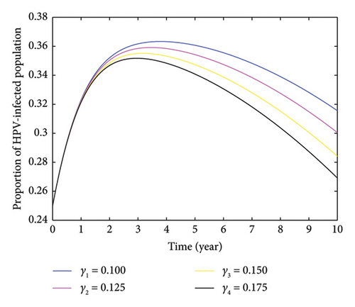
Based on the findings presented in Figure 9, when the value of the recovery rate was altered from γ1 = 0.100 to γ2 = 0.175, the value of R0 decreased from 3.5939 to 2.5085. It is evident that the value decreases as the rate of recovery of infected individuals increases. This implies that boosting the recovery rate can help in reducing the number of HPV-infected individuals, ultimately aiding in the decrease and elimination of cervical cancer within the community.
5. Discussion and Conclusion
In our research, we developed and analyzed a SVPIHPVCR mathematical model to study the spread of HPV and its impact on the dynamics of cervical cancer. In Section 3, we provided a detailed qualitative analysis of the model based on a system of differential equations derived from the model diagram. Our analysis confirmed that the model’s solution is well posed and positive. To assess the disease dynamics, we calculated the basic reproductive number using the next-generation matrix. Based on this reproductive number, we evaluated the local and global stability of disease-free and endemic equilibrium points. Our stability analysis revealed that the disease-free equilibrium point is locally asymptotically stable if the basic reproductive number is greater than one (determined using the Jacobian matrix).
We conducted a sensitivity analysis to understand the contribution of each basic parameter to the disease dynamics where their sensitivity indicators are expressed in Table 2. The analysis showed that the recruitment rate (π), contact rate (β), and waning out of the first vaccination rate (δ) have positive sensitivity indicators, meaning that increasing these parameters has the greatest impact on the spread of HPV and subsequently leads to increased cervical cancer cases. In contrast, the first-dose rate (α), second-dose rate (θ), and recovery rate (γ) have negative sensitivity indicators, indicating that increasing the value of these parameters and reducing those with positive sensitivity indicators can help minimize or eradicate the disease.
Following the theoretical and analytical parts, we performed numerical simulations to investigate the effects of the basic parameters. The results were graphically represented using MATLAB R2015a computer software. Utilizing the parameter values outlined in Table 3, we derived a numerical value for the average number of secondary infectious individuals caused by a single infectious person R0 = 2.7893. This value indicated that a single HPV-infected individual can, on average, transmit the infection to HPV-vulnerable individuals within 2.7893 units of time. Furthermore, increasing the values of key parameters, such as the contact rate, led to a rise in the number of secondary HPV-infected individuals. Specifically, the number changed from R0 = 0.7525 to R0 = 3.7626 when the contact rate varied from β1 = 0.15 to β4 = 0.75.
Overall, our simulation results suggest that increasing values of parameters such as α (first vaccination dose), θ (second vaccination dose), and γ (recovery rate) and decreasing values of β (contact rate) and δ (waning out of the effectiveness of the first vaccination dose rate) contribute to reducing the average number of secondary HPV-infected individuals. Our study emphasizes the importance of focusing on these parameters for predicting and controlling the dynamics of HPV and cervical cancer, particularly for healthcare professionals and policymakers worldwide.
Conflicts of Interest
The authors declare no conflicts of interest.
Funding
This study did not receive any funding.
Open Research
Data Availability Statement
The data used to support the findings of this study are obtained from published articles and are included within the article with due citation.


