Volume 2025, Issue 1 8553106
Research Article
Open Access

An Optimal Control Study for a Two-Strain SEIR Epidemic Model With Saturated Incidence Rates and Treatment

Karam Allali

Karam Allali

Laboratory of Mathematics , Computer Science and Applications , Faculty of Sciences and Technologies , University Hassan II of Casablanca , P.O. Box 146, Mohammedia , Morocco , univcasa.ma

Search for more papers by this author
Mouhamadou A. M. T. Balde

Corresponding Author

Mouhamadou A. M. T. Balde

Laboratory of Mathematics of Decision and Numerical Analysis , University of Cheikh Anta Diop , Dakar , Senegal , ucad.sn

Search for more papers by this author
Babacar M. Ndiaye

Babacar M. Ndiaye

Laboratory of Mathematics of Decision and Numerical Analysis , University of Cheikh Anta Diop , Dakar , Senegal , ucad.sn

Search for more papers by this author
First published: 21 April 2025
Citations: 1
Academic Editor: Ahmed Ezzat Matouk

Abstract

This work will study an optimal control problem describing the two-strain SEIR epidemic model. The model studied is in the form of six nonlinear differential equations illustrating the dynamics of the susceptible and the exposed, the infected, and the recovered individuals. The exposed and the infected compartments are each divided into two subclasses representing the first and the second strains. The model includes two saturated rates and two treatments for each strain. We begin our study by showing the well posedness of our problem. The basic reproduction number is calculated and depends mainly on the reproduction numbers of the first and second strains. The global stability of the disease-free equilibrium is fulfilled. The optimal control study is achieved by using the Pontryagin minimum principle. Numerical simulations have shown the importance of therapy in minimizing the infection’s effect. By administrating suitable therapies, the disease’s severity decreases considerably. The estimation of parameters as well as a comparison study with COVID-19 clinical data is fulfilled. It was shown that the mathematical model results fit well the clinical data. In order to eradicate the infection, it is very important that the first and second strain reproduction numbers must be less than unity.

1. Introduction

The SIR pioneer work of Kermack and McKendric in 1927 [1] has inaugurated most mathematical modeling in epidemiology. SIR abbreviation stands for susceptible-infected-recovered compartments. Those classes were sufficient to study many infectious diseases. However, after the infection occurs, the individual is first exposed to the virus and will be infectious. Therefore, another compartment must be added to the classical SIR one, and the new abbreviation will be SEIR, which means susceptible-exposed-infected-recovered configuration. Many papers have used the SEIR model to study many infectious diseases such as coronavirus disease 2019 (COVID-19) [2, 3], hepatitis B infection (HBV) [4], and human immunodeficiency virus (HIV) [5]. It is worthy to notice that the late COVID-19 has attracted the attention of many researchers [6]. Different treatments of infectious diseases have been considered and studied in many works [79]. The optimal control of many infectious diseases has been studied [1012].

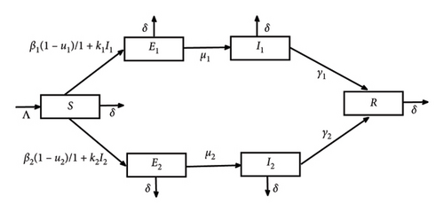
Mutation processes were noticed in many infections such as influenza, dengue fever, COVID-19, HIV, and tuberculosis [1317]. The mutation phenomenon is linked to the observation of the pathogen multiple strains. Consequently, mathematical models incorporating two or more strains are better for studying and understanding the evolution of many strains in a single disease case. The global dynamics of the multistrain SEIR epidemic model with an application to the COVID-19 pandemic was studied in [18]. More recently, the analysis and optimal control of a two-strain SEIR infection model was studied in [19]. The authors of the latter work have considered that the infected individuals may recover at a saturated treatment and studied the optimal control of the strategies undertaken. In this work, we will continue the investigation of the optimal control of two-strain epidemic problems by considering two controls for minimizing the force of infection. In practice, the two controls can represent the vaccination of the susceptible or social distancing between the susceptible and the infectious individuals. The dynamics of our two-strain epidemic model with treatments and saturated rate that describes the interaction between the susceptible denoted S(t), the strain-1 exposed individuals E1(t), the strain-2 exposed E2(t), the strain-1 infected I1(t), the strain-2 infected I2(t), and the recovered individuals are represented R(t) are given under the following form:
()
where the parameter Λ represents the recruitment rate of susceptibles through either birth or immigration, β1 (respectively, β2) is the strain-1 infection rate (respectively, the strain-2 infection rate). μ1 (respectively, μ2) is the strain-1 latency rate (respectively, the strain-2 latency rate). The parameter ki (i = 1, 2) measures the psychological, inhibitory, or crowding effect in the ith strain. γ2 = i (i = 1, 2) is the ith strain recovery rate. The natural mortality rate of the population is denoted by δ. Finally, the new parameters to the problem u1 and u2 represent the treatment efficiency for the first and the second strain, respectively. The two-strain diagram of the infection is illustrated in Figure 1. The estimation of parameters as well as a comparison study with COVID-19 clinical data is fulfilled. It was shown that the mathematical model results fit well the clinical data.
Details are in the caption following the image
The two-strain infection diagram.

The organization of this present paper will take the following form. First, Section 2 will be devoted to our two-strain SEIR epidemic model with two saturated incidence rates and two treatments. Next, Section 3 will investigate the disease-free equilibrium global stability. The optimal control study of our problem using the Pontryagin minimum principle is fulfilled in Section 4. Section 5 is dedicated to several numerical solutions showing the importance of the control strategy. Concluding remarks are given in Section 6. The parameters estimation is given in the Appendix section.

2. The Problem Well Posedness

In this section, we will focus attention on the problem’s well posedness. More precisely, we will show that Problem (1) admits a positive and bounded solution.

2.1. Positivity Results

Our problem describes population dynamics; therefore, all the acting variables must be nonnegative. Hence, we have the following result of positive invariance.

Theorem 1. For any initial data , the variables (S(t), E1(t), E2(t), I1(t), I2(t), R(t)) to Model (1) will remain also positive ∀ t > 0.

Proof 1. First, assume that tf = sup{ζ ≥ 0 | ∀t ∈ [0, ζ] we have S(t) ≥ 0, E1(t) ≥ 0, E2(t) ≥ 0, I1(t) ≥ 0, I2(t) ≥ 0and R(t) ≥ 0}. Let us now prove that tf = +.

Suppose that 0 < tf < +, then from the solutions continuity fact, we have S(tf) = 0 or E1(tf) = 0 or E2(tf) = 0 or I1(tf) = 0 or I2(tf) = 0 or R(tf) = 0.

Suppose that S(tf) = 0, then
()

However, from System (1) first equation, we have (dS(tf)/dt) = Λ > 0, which contradicts (2). Similar remark for the other variables E1(t), E2(t), I1(t), I2(t), and R(t). We conclude that tf could not be finite. This concludes the demonstration.

2.2. Boundedness Result

Proposition 1. The following closed set

()
is a positively invariant set.

Proof 2. Let the total population be

()

Adding all equations of (1) to each other, we have
()
and, therefore,
()
hence for t, we will have T(t) = Λ/δ.

We conclude that is a positively invariant set. All solutions to Problem (1) remain bounded.

The positivity and boundedness results ensure the existence of solution.

3. Analysis of the Problem

This section will be devoted to providing the basic reproduction number and the disease-free equilibrium stability result.

Since the first five equations of Problem (1) are independent of the last variable R, we can omit the last equation. Hence, we can study the following five equations reduced system:
()

3.1. Basic Reproduction Number

System (7) has a unique disease-free equilibrium given as follows:
()
The next generation matrix method in [20] will be used to calculate Problem (1) basic reproduction number . It is well known that we have
()
where ρ is the spectral radius, the matrix describes the new infections, and the matrix represents the transition terms.
()
So, is given as follows:
()
Hence, the basic reproduction number is given by
()
with
()

is called the strain-1 reproduction number, while is nemad the strain-2 reproduction number.

3.2. Global Stability of the Disease-free Equilibrium

We obtain the global stability of the disease-free equilibrium using the Lyapunov method. More precisely, we have the following result.

Theorem 2. The disease-free equilibrium is globally asymptotically stable when the basic reproduction number is less than unity.

Proof 3. First, let us consider the following Lyapunov function:

()

We remark that . The positivity of L comes from the fact that
()
Now, the time derivative of L(t) is given by
()
Then,
()
Hence, we have
()
which means that
()
Moreover, knowing that
()
It leads to
()

Finally, when and .

We conclude that the negativity of the Lyapunov function will be achieved when the basic reproduction number is less than unity.

The disease-free equilibrium is globally asymptotically stable when .

4. The Optimal Control Study

To study the optimal control, we will vary the two treatments u1 and u2 and seek the optimal pair to reduce the infection. The model with the varied controls becomes
()
where ui(t) ∈ [0, 1],  ∀ t ≥ 0.

4.1. The Infection Optimization Problem

Let the objective functional be maximized as follows:
()
where te represents the needed end-time for the treatment measures. The two positive constants C1 and C2 are based on the costs of each treatment strategy u1(t) and u2(t), respectively.
The principal objective is to find the right pair that allows reducing the infection severity. In other words, we will seek to maximize the susceptible and to minimize the costs.
()
under the constraints of (22), where U is the control set given by
()

4.2. Existence of Trajectories

Let us set x = (S(t), E1(t), E2(t), I1(t), I2(t), R(t)) and let us denote by the right-hand side of the differential equation model (22), with
()

Theorem 3. f satisfies the following equation:

()
where K1 and K2 are positive constants.

Proof 4. Since f(t, x, u) is at least C1 with respect to t,  x,  u and x,  u belong to the bounded set and U, respectively, then (12) is satisfied (see [21, 22]).

Theorem 4. For any control u(·) ∈ [0, 1]2, the ODE System (22) has a unique solution.

Proof 5. It is a consequence of the fact that (27) is satisfied (see [22]).

Theorem 5. There exists an optimal control pair solving the optimal control problem (22)–(24).

Proof 6. We exploit the existence theorem in [22] (Theorem III.4.1 p68-69).

By Theorem 3, we have that (27) is satisfied.

The set is clearly not empty by Theorem 4.

The set [0, 1]2 is convex and closed.

The running cost is convex on U. Indeed, the Hessian of L with respect to u is
()
Since C1 and C2 are strictly positive constant, we deduce the convexity of L on U.
()

Hence, L(t, x, u) ≥ c1uβc2, with c1 = C, c2 = Λ/δ and β = 2.

4.3. The Infection Optimality System

To apply Pontryagin’s minimum principle [23], we will need the following Hamiltonian under the following form:
()

The optimality system to Problem (22) is given by the following result.

Theorem 6. There exist six adjoint equations to Problem (22) given by

()
with the transversality conditions
()

The optimal controls are given by
()
()

Proof 7. The six adjoint equations can be obtained via Pontryagin principle [23] such that

()
with the transversality conditions
()

System (35) becomes (31).

The two optimal controls can be found by solving
()
This leads to
()
Since the two controls are in the interval [0, 1]. Therefore,
()

5. Numerical Simulations

In this section, we will provide some numerical simulations to highlight the role of control strategies in combating the infection. We use Gekko Optimization Suite [24] in Python [25]. Fitting data of the cumulative cases of Senegal country estimate the model’s parameters. For more details, see the Appendix. We consider T = 16743927 the total population of Senegal. We have two tests: Test 1 and Test 2. The values of the parameters are shown in Table 1.

Table 1. Values of parameters for different tests.
Parameters Test 1 Test 2
Λ 0.0914T/100 0.0914T/100 Fixed
k1 0.05 0.2 Fixed
k2 0.04 0.15 Fixed
δ 0.000219 0.000219 Fixed
ξ1 10 0.08 Fixed
ξ2 12 0.9 Fixed
μ1 0.00012 0.003 Fitted
μ2 0.001 4.896·10−5 Fitted
β1 7.71·10−7 1.52·10−6 Fitted
β2 7.92·10−7 4.6·10−6 Fitted
γ1 5.57·10−5 0.0009 Fitted
γ2 0.000515 0.0002 Fitted
C1 100/β2 100/β2 Fixed
C2 100/β1 100/β1 Fixed

Table 2 gives the initial conditions.

Table 2. Initial conditions.
Initial conditions S(0) E1(0) E2(0) I1(0) I2(0) R(0)
Test 1 16660213 20212 24254 17065 22184 0
Test 2 16661290 8085 40424 6826 27303 0

The parameters Λ, k1, k2, δ, ξ1, and ξ2 are fixed. By inserting them into the formulas in the Appendix, obtained by fitting the model to the COVID-19 data, we obtain the values of the other parameters as well as the initial conditions. Since for both tests, we choose different values of k1 and k2, we obtain different values of the fitted parameters and the initial conditions.

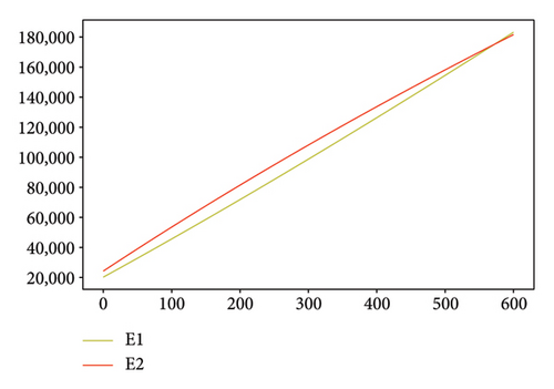
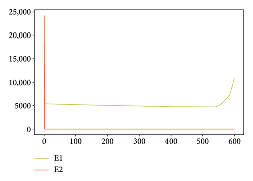
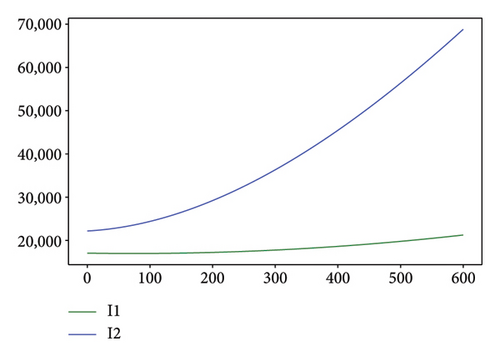
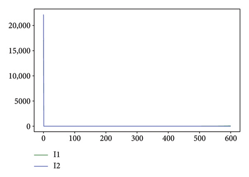
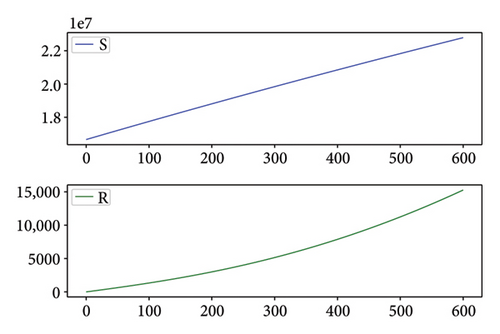
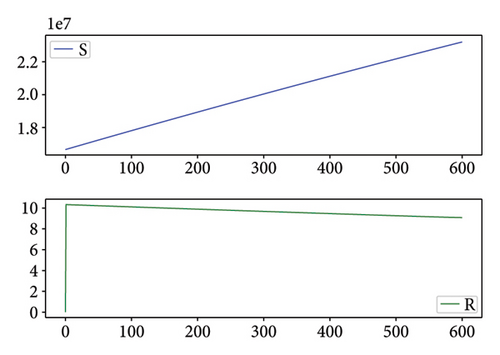
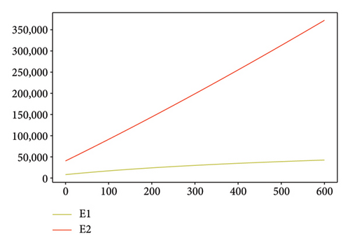
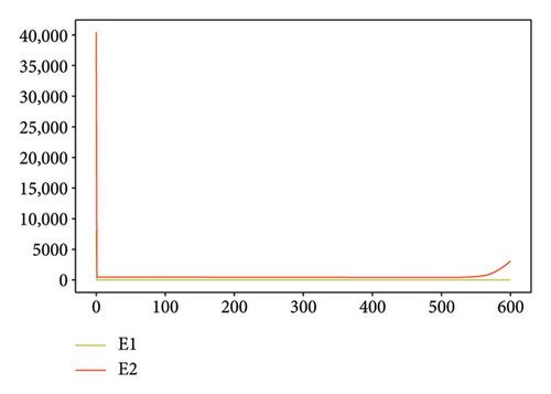
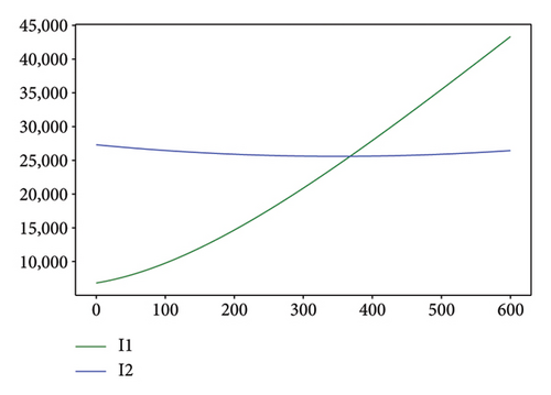
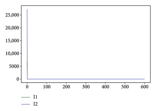
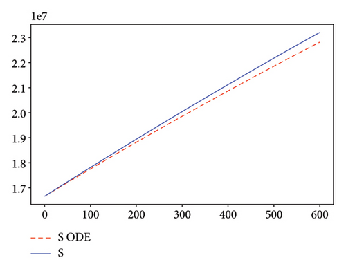
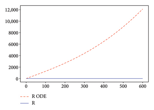
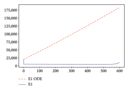
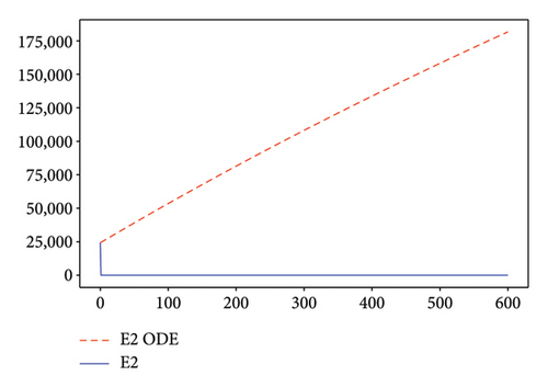
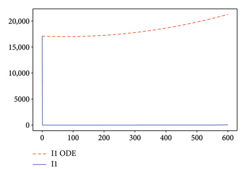
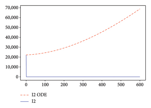
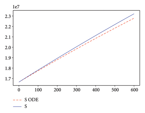
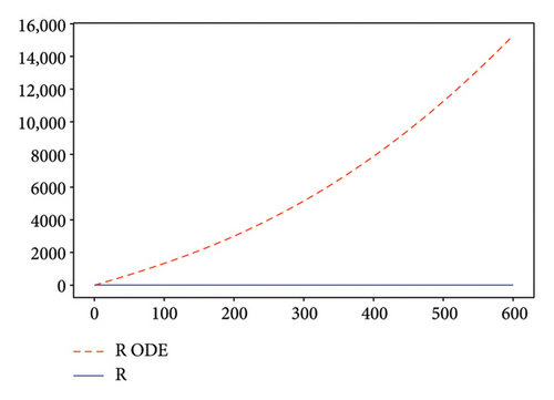
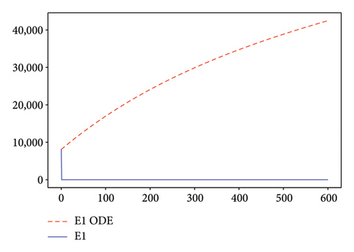
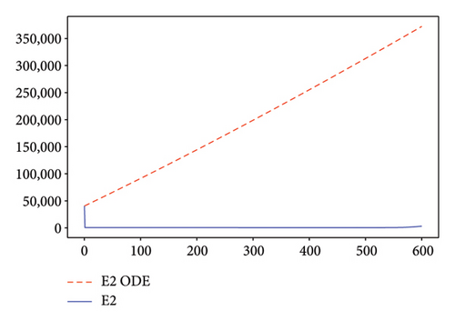
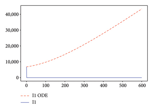
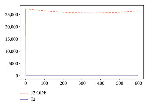
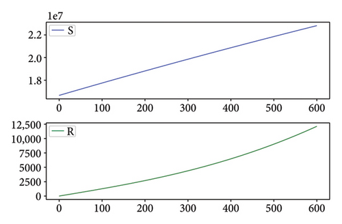
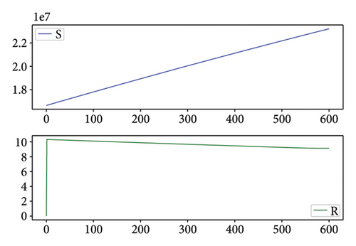
Figures 2, 3, 4, and 5 show the dynamic of two-strain infection model with and without controls. We clearly observe that with control, the number of susceptible individuals is higher than that without control. Hence, controls have played an essential role in maximizing susceptible individuals. Moreover, in both strains, infected and exposed individuals are reduced with control, while without the control, they remain at a strictly positive level. The convergence toward the free endemic equilibrium with control is observed. More precisely, all the states converge toward the endemic-free equilibrium (Λ/δ, 0, 0, 0, 0, 0), which means that the infection can be eradicated.
Details are in the caption following the image
Plot of states with and without controls of Test 1. (a) Susceptible S and recovered R cases without controls. (b) Susceptible S and recovered R cases with controls. (c) Exposed E1 and E2 without controls. (d) Exposed E1 and E2 with controls. (e) Infected I1 and I2 without controls. (f) Infected I1 and I2 with controls.
Details are in the caption following the image
Plot of states with and without controls of Test 2. (a) Susceptible S and recovered R cases without controls. (b) Susceptible S and recovered R cases with controls. (c) Exposed E1 and E2 without controls. (d) Exposed E1 and E2 with controls. (e) Infected I1 and I2 without controls. (f) Infected I1 and I2 with controls.
Details are in the caption following the image
Comparative plot of states with and without controls of Test 1 without controls in red dotted lines and with controls in blue lines. (a) Susceptible S. (b) Recovered R. (c) Exposed E1. (d) Exposed E2. (e) Infected I1. (f) Infected I2.
Details are in the caption following the image
Comparative plot of states with and without controls of Test 1 without controls in red dotted lines and with controls in blue lines. (a) Susceptible S. (b) Recovered R. (c) Exposed E1. (d) Exposed E2. (e) Infected I1. (f) Infected I2.
Details are in the caption following the image
Comparative plot of states with and without controls of Test 1 without controls in red dotted lines and with controls in blue lines. (a) Susceptible S. (b) Recovered R. (c) Exposed E1. (d) Exposed E2. (e) Infected I1. (f) Infected I2.
Details are in the caption following the image
Comparative plot of states with and without controls of Test 1 without controls in red dotted lines and with controls in blue lines. (a) Susceptible S. (b) Recovered R. (c) Exposed E1. (d) Exposed E2. (e) Infected I1. (f) Infected I2.
Details are in the caption following the image
Comparative plot of states with and without controls of Test 1 without controls in red dotted lines and with controls in blue lines. (a) Susceptible S. (b) Recovered R. (c) Exposed E1. (d) Exposed E2. (e) Infected I1. (f) Infected I2.
Details are in the caption following the image
Comparative plot of states with and without controls of Test 1 without controls in red dotted lines and with controls in blue lines. (a) Susceptible S. (b) Recovered R. (c) Exposed E1. (d) Exposed E2. (e) Infected I1. (f) Infected I2.
Details are in the caption following the image
Comparative plot of states with and without controls of Test 2 without controls in red dotted lines and with controls in blue lines. (a) Susceptible S. (b) Recovered R. (c) Exposed E1. (d) Exposed E2. (e) Infected I1. (f) Infected I2.
Details are in the caption following the image
Comparative plot of states with and without controls of Test 2 without controls in red dotted lines and with controls in blue lines. (a) Susceptible S. (b) Recovered R. (c) Exposed E1. (d) Exposed E2. (e) Infected I1. (f) Infected I2.
Details are in the caption following the image
Comparative plot of states with and without controls of Test 2 without controls in red dotted lines and with controls in blue lines. (a) Susceptible S. (b) Recovered R. (c) Exposed E1. (d) Exposed E2. (e) Infected I1. (f) Infected I2.
Details are in the caption following the image
Comparative plot of states with and without controls of Test 2 without controls in red dotted lines and with controls in blue lines. (a) Susceptible S. (b) Recovered R. (c) Exposed E1. (d) Exposed E2. (e) Infected I1. (f) Infected I2.
Details are in the caption following the image
Comparative plot of states with and without controls of Test 2 without controls in red dotted lines and with controls in blue lines. (a) Susceptible S. (b) Recovered R. (c) Exposed E1. (d) Exposed E2. (e) Infected I1. (f) Infected I2.
Details are in the caption following the image
Comparative plot of states with and without controls of Test 2 without controls in red dotted lines and with controls in blue lines. (a) Susceptible S. (b) Recovered R. (c) Exposed E1. (d) Exposed E2. (e) Infected I1. (f) Infected I2.

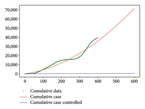
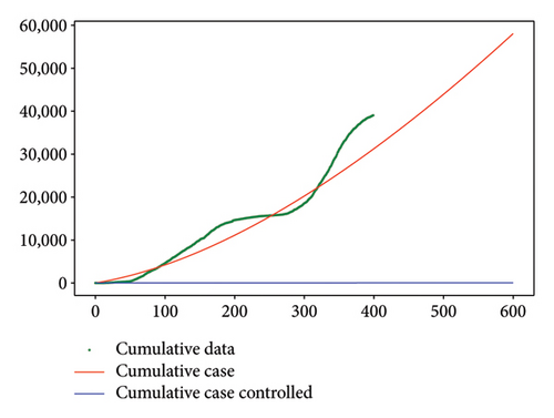
Figure 6 shows a comparison of cumulative case data, the cumulative case with and without controls.
Details are in the caption following the image
Plot of cumulative case. The COVID-19 cumulative case data are in green, the cumulative case without control is in red, and the minimal cumulative case is in blue. (a) Test 1. (b) Test 2.
Details are in the caption following the image
Plot of cumulative case. The COVID-19 cumulative case data are in green, the cumulative case without control is in red, and the minimal cumulative case is in blue. (a) Test 1. (b) Test 2.

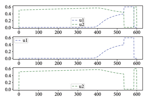
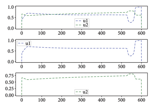
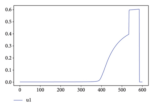
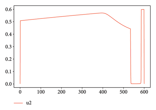
For Test 1, we see that from 0 to 400, the control u1 is zero unlike the control u2, which is at an average level over the period from 0 to 500 as is shown in Figure 7, while the trends are reversed in the period from 500 to 600. Thus, in the first period, the priority is given to the treatment of Strain 2 and the situation is reversed in other periods. This has made it possible to reduce the cumulative cases of infection as depicted in Figure 6(a).
Details are in the caption following the image
Plot of controls of Test 1. (a) Control u1. (b) Control u2. (c) Both controls u1 and u2.
Details are in the caption following the image
Plot of controls of Test 1. (a) Control u1. (b) Control u2. (c) Both controls u1 and u2.
Details are in the caption following the image
Plot of controls of Test 1. (a) Control u1. (b) Control u2. (c) Both controls u1 and u2.

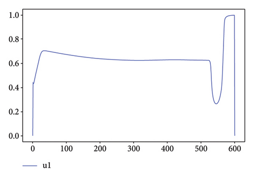
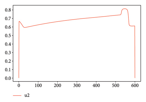
As shown in Figure 8 for Test 2, the controls u1 and u2 are at a high level, varying between 0.6 and 1 over most of the study period from 0 to 600. Indeed, control u1 has a level lower than 0.5 over the period from 525 to 575. Thus, over the periods from 0 to 20 and from 150 to 575, the priority is given to the treatment of Strain 2 unlike the other periods. We see that the cumulative case of infection is reduced over the entire study period as shown in Figure 6(b).
Details are in the caption following the image
Plot of controls of Test 2. (a) Control u1. (b) Control u2. (c) Both controls u1 and u2.
Details are in the caption following the image
Plot of controls of Test 2. (a) Control u1. (b) Control u2. (c) Both controls u1 and u2.
Details are in the caption following the image
Plot of controls of Test 2. (a) Control u1. (b) Control u2. (c) Both controls u1 and u2.

6. Conclusion

In this work, we have studied numerically and theoretically a mathematical model describing the dynamics of a two-strain SEIR epidemic model. The model contains a system of nonlinear differential equations describing the interaction between the susceptible, the first, and the second strain exposed individuals, the first and the second strain infected individuals and the recovered ones. Two saturated rates and two treatments were incorporated into the model. The well posedness of the model was established in terms of positivity and boundedness of solutions. The basic reproduction number was calculated as a function of the reproduction numbers of the first and second strains. The global stability of the disease-free equilibrium was fulfilled. We have performed an estimation study of the problem parameters. In addition, the model numerical simulation was compared with COVID-19 clinical data. The optimal control study was achieved by using the Pontryagin minimum principle. Numerical simulations have shown the importance of therapy in minimizing the infection’s effect. It was shown that the disease severity decreased remarkably when good therapies were administrated. As future directions of the present work, one can consider more than two strains or include the birth logistic growth rate.

Disclosure

A preprint of this paper was shared in Arxiv on April 26, 2024 [29].

Conflicts of Interest

The authors declare no conflicts of interest.

Funding

No funding was received for this work.

Acknowledgments

Karam Allali is grateful to the support from the Laboratory Mathematics, Computer Science and Applications, University Hassan II of Casablanca and the hospitality of Babacar Mbaye Ndiaye at LMDAN in the University Cheikh Anta Diop of Dakar during the research collaboration visit.

    Appendix A: Estimation of Parameters

    The estimation of the parameters of Model (1) is done by using the techniques in [21, 26, 27]. Generally, pandemic data fit with an exponential type of function. Analyzing the Senegal COVID − 19 data, we see that the function does not follow exponential curve.

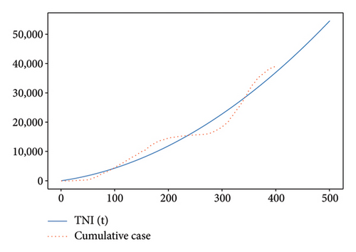
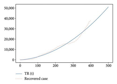
    We fit, respectively, the cumulative and recovered case data of COVID − 19 in Senegal, from 2020 March 02 to 2021 April 04, with the two polynomial functions TNI(t) = at2 + bt + c and TR(t) = et2 + ft + g, see Figure A1. In addition, we assume that these functions can be given in integral form as and .
    Details are in the caption following the image
    Fit of cumulative cases and recovered data from March 02, 2020, to April 04, 2021. (a) Cumulative case data in red and fit function TNI (t) in blue. (b) Recovered case data in red and fit function TR (t) in blue.
    Details are in the caption following the image
    Fit of cumulative cases and recovered data from March 02, 2020, to April 04, 2021. (a) Cumulative case data in red and fit function TNI (t) in blue. (b) Recovered case data in red and fit function TR (t) in blue.
    Deriving TNI gives
    ()
    We suppose that μ2E2,0 = ξ1μ1E1,0, implying (1 + ξ1)μ1E1,0 = b. Then,
    ()
    Deriving again, we obtain
    ()
    Supposing that , we obtain . We get
    ()
    Some calculations give
    ()
    Deriving TR(t) gives
    ()
    We suppose that γ2I2,0 = ξ2γ1I1,0. Doing the same work as above, we obtain
    ()
    Using the second equation of Model (1) and setting u1 = u2 = 0, we obtain
    ()
    Using again the third equation of Model (1) and doing the same work as above give
    ()

    We use 32.9% of year 2018 for the birth rate from [28]. Then, the recruitment is Λ = 32.9%T/365 by day. The death rate is 7.9% by the year 2018.

    Now, we will discuss the coefficients C1 and C2. We simulated two tests. For both tests, the values of the coefficients are related to the infection rate. We consider that if the infection rate is such that β1 < β2, then the propagation of Strain 2 is more than that of Strain 1. The more the infection spreads through the population, the greater the treatment expenses. Then, we set C1 = 100/β2 and C2 = 100/β1.

    Data Availability Statement

    Data sharing not applicable to this article as no datasets were generated or analyzed during the current study.

      The full text of this article hosted at iucr.org is unavailable due to technical difficulties.