The dynamic latent space model is widely used in analysing network data. It can provide useful visualization and interpretation of networks, as well as represent the inherent reciprocity and transitivity. In this paper, a dynamic latent space model with position clusters is proposed. The model extends the dynamic latent space model by incorporating latent position clustering and accounting for weighted networks. A fully Bayesian method with adaptive Markov chain Monte Carlo sampling is used to estimate the novel model. A purity-based relabelling algorithm is proposed to resolve label switching. This model can be extended to analyse binary networks, count networks and sparse weighted networks. Finally, the model is used to analyse the product trade data of 54 countries from 2010 to 2019.

1. Introduction

Network data describe the relationships between actors that widely exist in various fields of social life. Static network data with n individuals are typically represented as , and dynamic network data are represented as , where T is the time span. For example, in the Weibo network, y_ij represents whether the ith person’s Weibo accounts for the jth person’s Weibo, and are binary network data [1]. In the international trade network, y_ijt represents the trade volume exported from country i to country j in year t, and are continuous network data [2]. In recent years, research on statistical modelling for network data has increased [3–5].

The features of most networks are reciprocal (if there is a strong relation from i to j, then generally there is also a strong relation from j to i), transitive (if the relations between i and j, j and k are strong, then i and k generally have a strong relation) and clustered (actors in the same group have stronger relations, while actors in different groups have weaker relations, or actors in the same group have similar characteristics, and so on). Therefore, the statistical modelling of network data needs to comprehensively consider the above properties.

Exponential random graph models (ERGMs) are a broad class of network models that are very popular in the social sciences [6]. ERGMs have been designed to account for transitivity and reciprocity. However, ERGMs are not well understood, they possess undesirable degeneracy, their likelihood function can be intractable, and some unobserved structures may be omitted [3]. Therefore, latent variable models built on conditional independence, such as stochastic block models (SBMs) and latent space models (LSMs), have attracted much attention.

Researchers are often interested in clustering network actors. Early studies on network clustering mainly focussed on community detection, where actors in the same class were closely connected, while actors in different classes were distantly connected, such as through spectral clustering methods [7]. To achieve more general clustering, researchers have proposed methods based on statistical models. Lorrain and White [8] developed the concept of structural equivalence. Holland, Laskey, and Leinhardt [9] developed a probabilistic model for the stochastic equivalence of actors in a network, under which the probabilities of relationships with all the other actors are the same for all the actors in the same class. Snijders and Nowicki [10], Nowicki and Snijders [11] extended this model to latent classes in which the clustering memberships are assumed to be unknown and need to be estimated from the data, that is, they are SBMs. Matias and Miele [12] explored dynamic SBMs. These models capture some kinds of clustering, but they do not represent transitivity, and neglect the local structure of the network.

The idea of LSMs is to reflect network information in a low-dimensional latent space. The static LSM of Hoff, Raftery, and Handcock [13] is a stochastic model of the network in which each actor has a latent position in a Euclidean space or on a unit hypersphere. The latent positions are estimated by using standard statistical principles. In the dynamic latent space (DLS) approach of Sewell and Chen [14], the network time series can be represented as a state space model, with the latent state variable representing the actors as positions in a low-dimensional Euclidean space. The closer two actors are in this latent Euclidean space, the more likely they are to form an edge. This low-dimensional space can be thought of as a characteristic space where the distance between actors represents how similar they are. This type of model has many advantages, both the local and global structures are modelled, and transitivity and reciprocity are inherently incorporated into the model, meaningful visualizations are obtained, and the outputs are easily interpreted. Therefore, LSMs have received much attention [4, 15–17]. However, the approach of Sewell and Chen [14] cannot achieve clustering of network actors nor analyse nonbinary weighted networks. Handcock, Raftery, and Tantrum [18] have considered the clustering of latent positions in static LSMs, while Sewell and Chen [19], Casarin and Peruzzi [20], and Daniel Loyal and Chen [21] have addressed the clustering of latent positions in DLS models. Although they accommodate clustering, these models have failed to simultaneously consider clustering, weighted networks, and the different effects of the receiver and the sender in directed networks.

Here, we propose a new model, the DLS model with position clusters (DLS-PC). This model extends the DLS model of Sewell and Chen [14] to incorporate clustering, using the ideas of model-based clustering. It naturally considers the reciprocity, transitivity and clustering in a unified framework. Moreover, the model can be applied to weighted networks and is capable of analysing the different effects of senders and receivers within directed networks.

The remainder of the article is organized as follows. Section 2 describes the proposed model. Section 3 explores Bayesian estimation, as well as the issues of identification, label switching and model selection. Section 4 shows the simulation results. Section 5 presents the results from analysing international trade data. Section 6 provides a brief discussion.

2. DLS-PC

To model binary dynamic network data

, Sewell and Chen [14] proposed a DLS model,

()

where

()

In model (1), Y_t = {y_ijt} is the adjacency matrix of the observed network at time t. y_ijt = 1 indicates that there is an edge from actor i to actor j, and y_ijt = 0 is the opposite. x_it is the K-dimensional vector of the ith actor’s latent position at time t. The latent position variables

and t = 1, …, T are modelled by a Markov process with the initial distribution

()

and the transition equation

()

for t = 2, …, T, where I is the identity matrix with compatible dimensions and ψ = (β_IN, β_OUT, r_1:n, τ², δ²) are model parameters.

This model yields a meaningful visualization of dynamic networks, providing researchers with insight into the evolution and structure, both local and global, of the network. The model can handle directed or undirected binary network data, and can reflect inherent reciprocity and transitivity. However, this model cannot achieve clustering of network actors. Other DLS models with clustering have also failed to simultaneously consider clustering, weighted networks, and the different effect of the receiver and the sender in directed networks [19–21].

Clustering actors is also an important topic in network analysing. By extending the DLS model of Sewell and Chen [14] to consider clustering, using the ideas of model-based clustering, we propose a DLS-PC,

()

where

()

The initial distribution of latent position variables is

()

the transitive equation is

()

where

()

Additionally, (C₁, …, C_n) are the cluster labels for the actors. We assume that the labels of actors are independent, and each follows a discrete probability distribution, that is

()

where p(C_i|ψ) is the distribution over actor i’s cluster assignments. The support of C_i is {1, …, G}, and P(C_i = g|ψ) is the probability that i belongs to class g. To avoid introducing too many parameters, we assume that C_i has a discrete uniform distribution in the subsequent research, that is, P(C_i = g|ψ) = 1/G [22].

The radii r_i’s are positive actor-specific parameters that represent each actor’s reach. For model identifiability, r_i’s are constrained so that .

β_IN > 0 and β_OUT > 0 are global parameters. If β_IN > β_OUT, then the strength of the relationship from i to j is determined more by the radius of j than by i. Thus, the network is determined more by the popularity of the actors than by their activity. That is, the identity of the receiver is more important than the identity of the sender in a network. β_IN < β_OUT is the opposite. Furthermore, when ‖x_it − x_jt‖ equals zero, we can obtain

()

which is the maximum possible value of E(y_ijt|X₁, …, X_T, C₁, …, C_n, ψ). This indicates that β_IN + β_OUT is the maximum expected connectivity strength. In a binary graph, density is defined as the ratio of the number of edges present to the maximum possible that could arise. Another way to view the density of a graph is as the average of the values assigned to the edges. To generalize the notion of density to a weighted graph, one can average the values attached to the edges [23]. Thus, under the latent space framework, the network density is (∑_i≠jη_ijt/n(n − 1)), which is less than the maximum density of the network (n(n − 1)(β_IN + β_OUT))/(n(n − 1)) = β_IN + β_OUT. On this basis, we can refer to (∑_i≠jη_ijt)/(n(n − 1)(β_IN + β_OUT)) as the realized density ratio at time t.

The idea of this model is that the dynamic network is represented by a state space model, with the latent state variables representing the positions of the actors in a low-dimensional Euclidean space. The closer two actors are in this Euclidean space, the stronger their relationship is in the network. We then assume that the relation between two actors is independent of all other relations, given their positions and radii. Additionally, to explore the clustering characteristics of the network, the DLS-PC model assumes that the mean vector and variance in each dimension of the initial positions, as well as the variance of the transitive equation, for actor i, are determined by the class to which i belongs.

Model (5) is suitable for continuous networks. For example, in the field of international trade, y_ijt represents the import trade volume of country j from country i at time t, and y_ijt is a continuous random variable. Model (5) can be extended to analyse binary networks, count networks [24] and sparse weighted networks [12].

For binary data, logistic regression is considered,

()

That is, y_ijt follows a Bernoulli distribution, and E(y_ijt|η_ijt) = (exp(η_ijt))/(1 + exp(η_ijt)).

For count data, Poisson regression is considered,

()

That is, y_ijt follows a Poisson distribution, and E(y_ijt|η_ijt) = exp(η_ijt).

For a sparse weighted network, Matias and Miele [12] introduced a Dirac mass at 0, so

()

where f(y_ijt|η_ijt, ψ) is a density (with respect to the Lebesgue or counting measure) with no point mass at 0. In the above three equations, ψ is a parameter vector,

is the indicator function.

3. Estimation

3.1. Markov Chain Monte Carlo (MCMC) Sampling

We adopt a Bayesian approach to estimate the DLS-PC model, and hence, we wish to make inferences based on

()

where

is a prior distribution,

()

can be obtained from model (5). This paper only estimates the continuous network, and the estimation methods for models (12)–(14) can be modified based on this paper by referring to Sewell and Chen [14, 24].

We set priors on the parameters as follows. The priors of β_IN, β_OUT, σ², r_1:n, μ₁, …, μ_G, , and are independent. The priors of β_IN, β_OUT, and σ² are improper priors, which are , , and . The prior of r_1:n is a Dirichlet distribution, that is, p(r_1:n) = Dirichlet(1). The prior of μ_g(g = 1, …, G) follows a multivariate normal distribution, that is, , where is a hyperparameter. The priors of and (g = 1, …, G) are both inverse gamma distributions, that is, and , and and are hyperparameters. Here, 1 is a vector with compatible dimensions where all the elements are 1, 0 is a vector with compatible dimensions where all the elements are 0.

By substituting the above prior distributions into equation (15), we can obtain

()

where η_ijt = β_IN(1 − (‖x_it − x_jt‖)/r_j) + β_OUT(1 − (‖x_it − x_jt‖)/r_i).

Because it is impossible to obtain the analytical expression for the posterior marginal distributions of the variables to be estimated from formula (17), we use the MCMC method to draw samples from the posterior distribution and further obtain Bayesian estimators.

The number of MCMC iterations required to reach convergence can be greatly reduced by setting appropriate initial values. The initial values in this article are obtained as follows:

1.
Construct binary network (A_ijt), where
()
2.
The initial radius values are set
()
3.
The initial value of the latent position X₁ is calculated via classical multidimensional scaling (CMDS), and the initial values of X₂, …, X_T can be obtained via generalized multidimensional scaling (GMDS, [25]). GMDS balances the positions from the previous time point with the CMDS result obtained at time t. The dissimilarity matrix is D_ijt, whose definition is
()
where (S_ijt) is the length of the shortest path from actor i to actor j calculated based on (A_ijt);
4.
The initial values of β_IN, β_OUT, and σ² can be calculated via the maximum likelihood method;
5.
Assume , , , and their initial values are calculated by the maximum likelihood method based on X₁, …, X_T.
6.
are obtained by sampling from the discrete uniform distribution.

After having the samples

of the lth round, we draw samples Ψ^{(l + 1)} by Metropolis-Hastings within the Gibbs algorithm [26]. Specifically,

Step 1: Draw β_IN from a truncated normal distribution.
Step 2: Draw β_OUT from a truncated normal distribution.
Step 3: Draw σ² from an inverse Gamma distribution.
Step 4: Draw r_1:n via the Metropolis-Hastings algorithm, and the proposal distribution is the Dirichlet distribution , where is a large number.
Step 5: Draw μ₁, …, μ_G from normal distributions sequentially.
Step 6: Draw from inverse Gamma distributions sequentially.
Step 7: Draw from inverse Gamma distributions sequentially.
Step 8: Draw C₁, …, C_n from the sampling probabilities sequentially.
Step 9: Draw X₁₁, …, X_1T, X₂₁, …, X_2T, …, X_nT by the Metropolis–Hastings algorithm sequentially, and the proposal distribution is a normal random walk.

Additionally, when drawing samples of latent positions and radii, we use an adaptive algorithm to determine the variance and in the proposal distributions. Referring to the method of Roberts and Rosenthal [27], we set up variables (logarithm of variance) and (). After the th batch of 50 iterations, we update the variables and by adding or subtracting an adaptation amount . The adaptation attempts to make the acceptance rate of the proposals as close as possible to 0.234, which is a universal optimal value [28].

3.2. Identification

It is also important to note the issues of identifying latent positions and classified labels. Due to the latent positions appearing in the model in the form of a Euclidean distance, the posterior remains unchanged for the rotation and reflection of the latent positions. Here, we can perform a Procrustes transformation to reorient the sampled trajectories [14, 29]. The Procrustes transformation on using as the target matrix finds , where is a rotation or reflection of . Therefore, before performing a posterior mean calculation, it is necessary to reorient the samples of the latent positions and the mean of the initial positions .

In addition, label switching describes the invariance of the likelihood under relabelling, which means that the posterior distribution remains unchanged for the permutations in the labelling [30]. Here, we propose a label estimation method that combines permutation sampling and label switching based on purity. That is, each sweep of the MCMC chain is concluded by relabelling the states through a random permutation of {1, …, G} [31]. This method delivers a sample that explores the entire unconstrained parameter space and jumps between the various labelling subspaces in a balanced fashion. Purity is a simple and transparent evaluation measure for clustering. The method involves assigning each cluster to the class that is most frequent within it, and then measuring the accuracy of this assignment by counting the number of correctly assigned instances [32]. When obtaining estimates, we permute the labels again using a method based on purity calculations. This method involves relabelling the samples so that the new labels most closely match certain target labels. The detailed algorithm is in Table 1, where is the set of actors belonging to class j before relabelling, is the set of actors belonging to class j after relabelling, is the set of actors belonging to class j for a certain target, and |Λ| is the number of elements in set Λ.

Table 1. The proposed purity-based relabelling algorithm.

Purity-based relabelling algorithm

1. Calculate for k, j = 1, …, G;
2. Relabel actors:
i. Find the g-th column where the maximum value is located in matrix C = (c_kj) (if there is more than one maximum value, choose the one with a smaller column number), and then find the row where the maximum value is located in g-th column (if there is more than one maximum value, choose the one with a smaller row number);
ii. Relabel the actors belonging class as g;
iii. Update accordingly;
iv. Exclude row and columns g, repeat the above operation until all actors obtain new labels.

3.3. Posterior Estimation

3.3.1. Maximum a Posteriori (MAP) Estimation

Assuming that Ψ⁽¹⁾, …, Ψ^(L) are the MCMC samples after the burn-in period, all the variables can be estimated using the posterior mode, MAP, that is,

()

3.3.2. Posterior Mean Estimation

Assuming that Ψ⁽¹⁾, …, Ψ^(H) are the MCMC samples after the burn-in period, thinning, reorientation and relabelling (the target positions are the initial positions of the MCMC chain, and the target labels are the MAP estimations), any continuous components in Ψ can be estimated by its posterior mean, that is,

. The discrete variables C_i’s can be estimated using the maximum sample posterior probability, that is,

()

3.4. Model Selection

As described in the previous section, we assume that G, the number of clusters, is correctly specified. Therefore, a fully Bayesian analysis would naturally call for model selection procedures to determine G. Here, we use posterior , where are the estimations of the latent positions, and choose the value of G that gives the largest value of [18, 33]. One of the reasons for taking this approach is that in a LSM, it makes sense to evaluate the specific configuration of the latent positions that will be used, rather than an average over the distribution of the latent positions.

Assigning equal prior probabilities to the models that are considered, the posterior is

()

where

and

. In addition,

is the integrated likelihood of the observations conditional on the latent positions, and

is the integrated likelihood of the latent positions. These integrals can be approximated by using the BIC approximation [34], that is,

()

where d₁ is the dimension of ψ₁, d₂ is the dimension of ψ₂, n_Y is the number of observations and n_X is the dimension of

is the estimate of ψ₁, and

is the estimate of ψ₂.

Therefore, the final approximation, the integrated BIC (IBIC), is

()

We seek a model with the minimum IBIC as the final model.

3.5. Prediction

Predicting future relations is an important and interesting problem. When considering prediction in the latent space context, it is of interest to predict both Y_T+1 and X_T+1. We use the following method to predict them.

()

Additionally,

()

where

()

Therefore,

()

4. Simulation

4.1. Monte Carlo Simulation Setup

In the simulation study, we focus on the performance of the proposed Bayesian MCMC algorithm for DLS-PC. Twenty datasets were simulated, each with the number of actors n = 60 and the number of time points T = 10, and the number of clusters is G = 3. The data generating process is

()

where ε_ijt(i ≠ j; t = 1, …, T) are independent and identically distributed with N(0, 1), and the latent positions x_it(i = 1, …, n; t = 1, …, T) are drawn by

()

μ_g(g = 1, …, G) were drawn from a multivariate normal distribution N(0, (1/n²)I) and C_i(i = 1, …, n) were drawn from a discrete uniform distribution, that is, P(C_i = g) = 1/G. Additionally,

and

are drawn from a Dirichlet distribution with parameter (10 × 1)^′.

4.2. Simulation Results

The root mean square error (RMSE) is used to evaluate the estimation results of β_IN, β_OUT, and σ², that is,

()

where M is the total number of simulations, ξ is the true value and

is the estimated value for the mth simulation.

Table 2 summarizes the estimated results using the DLS-PC model with G = 3. The mean, standard deviation and RMSE of , , and are listed. We then see that both the posterior mean and posterior mode did quite well at estimating the true values of β_IN, β_OUT, and σ², and the posterior mean performed better.

Table 2. Estimated results of β_IN, β_OUT, and σ².

Method	Mean	Standard deviation	RMSE
Posterior mean	1.0005	0.0084	0.0084
	1.9925	0.0147	0.0165
	1.0018	0.0084	0.0086

Posterior mode	1.0033	0.0146	0.0150
	1.9907	0.0218	0.0237
	1.0015	0.0118	0.0119

Note: The true values are β_IN = 1, β_OUT = 2 and σ² = 1.

To evaluate the estimated results of the latent positions X₁, …, X_T, the pairwise distances from the estimated latent positions and the pairwise distances from the true latent positions were compared. That is, for each (i, j), we can look at

()

giving us Tn(n − 1)/2 ratios for each simulation, where {x_it : i = 1, …, n; t = 1, …, T} are the true positions and

are the estimated positions. Figure 1 shows, for each simulation, a smoothed curve of the distribution of these ratios. The left panel shows the posterior mean, and the right panel shows the posterior mode. Notice that all these distributions are narrow and centred on 1, implying that the latent positions from the posterior mean and posterior mode are close to the truth, and the curves from the posterior mean are slightly greater. Therefore, the posterior means are ultimately used.

Details are in the caption following the image — **Figure 1 (a)**
Open in figure viewer PowerPoint

For the distribution of pairwise distance ratios, the estimated latent positions are compared with the true latent positions, and each curve corresponds to a simulation. (a) Shows the posterior mean, and (b) shows the posterior mode.

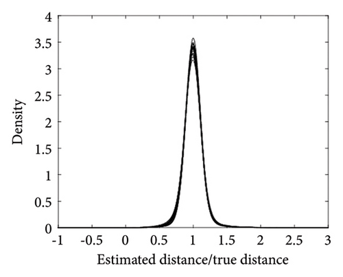
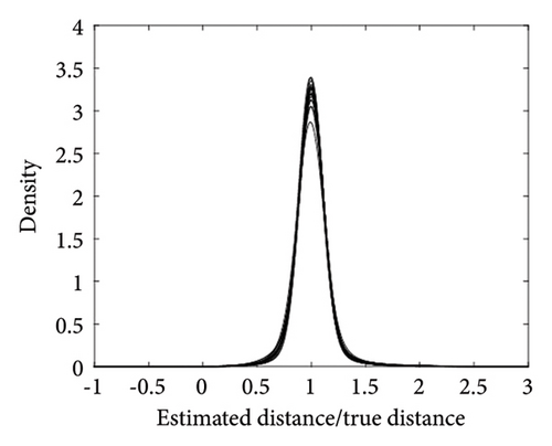
The performance of the estimated results for the radii can be evaluated using the absolute deviation. That is, we can calculate for all the actors in each simulation. Figure 2 shows a boxplot of these absolute deviations for each simulation. All the values are quite close to 0, indicating an excellent performance of the posterior mean.

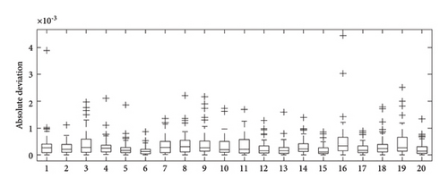
Table 3 lists the accuracy of clustering based on the maximum sample posterior probabilities in 20 simulations. It can be seen that, out of 20 simulations, 11 had accuracies of 100% for clustering. There are seven simulations where the accuracies are greater than 95%, and only two simulations where the results are not good, which are less than 95%, specifically, they are 93% and 82%.

Table 3. Correct proportion of clustering.

Accuracy	Number of times
100%	11
≥95% and 〈100%	7
〈95%	2

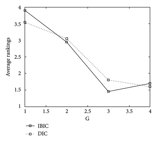
Figure 3 shows the model selection results for detecting the number of clusters by IBIC and DIC. The vertical axis represents the average rankings over 20 simulations. Thus, the IBIC method is better.

5. International Trade Network Analysis

Trade networks can better present the interconnection and dependence characteristics between countries, and have become a popular topic in the field of economics [35–37]. Increasing attention has been given to the study of the features of trade networks by statistical modelling. This paper further analyses the international trade network based on the DLS-PC model.

5.1. Data Description

The dataset for this study consists of a panel of 54 countries covering the period 2010–2019. These 54 countries had the largest import trade volumes during this period (excluding countries with missing data) and accounted for more than 85% of the world’s total imports. The countries and their serial numbers used in this paper are listed in Appendix A. The trade data come from the International Trade Centre (ITC). Most researchers regard import statistics as more reliable than export statistics since countries have a strong incentive to track the goods entering their country [38]. Therefore, y_ijt is the logarithm of the import volume plus 1 from country i at time t reported by country j. The data were collected by the United Nations Statistics Division and converted to US dollars (using the 2010 value as a constant), and the unit is thousands of dollars.

5.2. Empirical Results

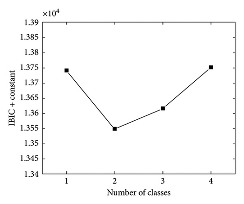
In this section, we use the DLS-PC model based on G = 1, G = 2, G = 3, and G = 4 to analyse international trade data. The Bayesian MCMC sampler is applied to estimate the DLS-PC model. A burn-in of 400,000 iterations was removed, leaving a chain of length 600,000. Thinning is performed by recovering only every 100th iteration. Additionally, a short MCMC chain with no clustering is used to initialize the latent positions. Figure 4 shows the IBICs of all the candidate models. The IBIC of G = 2 is the smallest. Therefore, we finally analyse the international trade data based on the DLS-PC model with G = 2 in the following text. In addition, we used the Ljung-Box Q-test to evaluate the independence of the residuals. The results showed that among the 2862 (54 ∗ 53) residual time sequences, only 10 exhibited p values below 0.01, and no sequence had a p value less than 0.005. That is, at the 0.005 significance level, we cannot reject the null hypothesis that the residual sequences are not autocorrelated. Consequently, it can be concluded that the time-series information has been fully extracted.

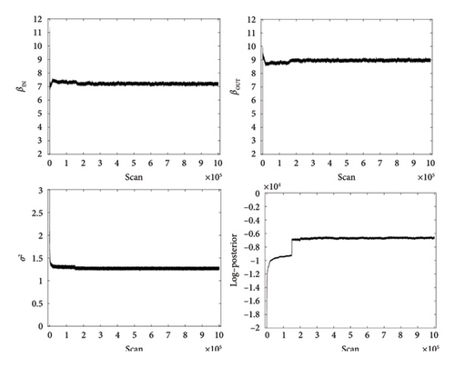
The trace plots of β_IN, β_OUT, σ², and log-posterior are shown in Figure 5 to demonstrate the convergence of the MCMC sampler. Table 4 shows the estimated results and confidence intervals of the parameters β_IN and β_OUT. β_OUT is slightly greater than β_IN. Therefore, international trade from country i to j is determined more by the radius of i than by that of j. The international trade network is determined more by the activity of countries, and the identities of export countries are more important than those of import countries. Moreover, β_IN + β_OUT = 16.1736, this indicates that the maximum network density is 16.1736. The network densities for these years are 13.2344, 13.2483, 13.2470, 13.2337, 13.2195, 13.2213, 13.2376, 13.2634, 13.2806, 13.2668. The corresponding realized density ratio are 0.8183, 0.8191, 0.8191, 0.8182, 0.8173, 0.8175, 0.8185, 0.8201, 0.8211, 0.8203. These ratios are closely clustered around 0.82, with 2018 showing the highest ratio and 2014 the lowest.

Table 4. Estimates of β_IN and β_OUT.

	Posterior mean	95% Confidence interval
	7.2080	(7.1142, 7.3014)
	8.9656	(8.8723, 9.0581)

Table 5 shows the radius estimations of all the countries. The radii of China, the United States of America, and Germany are larger than 0.1, and these countries have wide influences on the international trade network. The radii of Japan, the Russian Federation, Republic of Korea, France, Italy, United Kingdom, Netherlands, India, and Viet Nam are greater than 0.01. Other countries have smaller radii. To further investigate the relation between the radius and national attributes, this article explores two specific relationships during the sample period: one is between estimated radii and total import trade volumes, and the other is between radii and total GDP (constant in 2015 US dollars). This article calculates the correlation coefficients between the radius and total trade volume, as well as between the radius and GDP. Because the trade volumes and radii of China, United States of America, Germany, far exceeded those of other countries, these three countries were excluded from the calculation of the correlation coefficient. After calculation, the correlation coefficient between the radius and total trade is 0.5932, and the correlation coefficient between the radius and GDP is 0.6758. Therefore, generally speaking, countries with a large GDP often have a larger radius and a wider range of influence in the trade network.

Table 5. Radius estimations of countries.

Radii	Countries
≥0.1	10, 53, 17
≥0.01 and 〈0.1	25, 41, 27, 16, 24, 52, 32, 20, 54
〈0.01	49, 29, 47, 15, 43, 21, 37, 5, 46, 38, 6, 13, 34, 2, 50, 48, 8, 51, 33, 4, 3, 12, 28, 35, 26, 9, 22, 30, 42, 19, 1, 36, 23, 44, 45, 40, 11, 18, 14, 7, 39, 31

Note: Numbers represent the country’s serial number.

Table 6 shows the clustering results of countries. The countries classified into the second class are Iran, Viet Nam, and Belarus. The variances of the latent positions of these three countries are much larger than those of other countries. Except for these three countries, the other countries do not show obvious classification characteristics.

Table 6. Clustering results of all countries.

Class 1	1, 2, 3, 5, 6, 7, 8, 9, 10, 11, 12, 13, 14, 15, 16, 17, 18, 19, 20, 21, 23, 24, 25, 26, 27, 28, 29, 30, 31, 32, 33, 34, 35, 36, 37, 38, 39, 40, 41, 42, 43, 44, 45, 46, 47, 48, 49, 50, 51, 52, 53
Class 2	4, 22, 54

Note: Numbers represent the country’s serial number, and , , , .

Figure 6 shows the posterior means of the latent positions for each country in 2010 and 2019. The number is the serial number of the country in Table A1. The countries with red numbers belong to the first class, and the countries with blue numbers belong to the second class. The diamonds represent the means of the initial positions for the different classes. From 2010 to 2019, the latent positions of countries in the trade network did not change much. Countries classified in the second class are located on the periphery of the network.

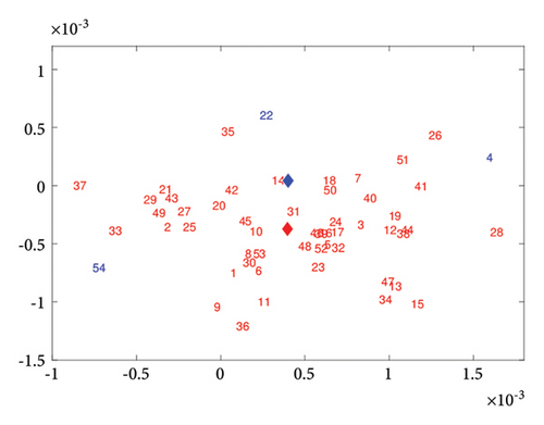
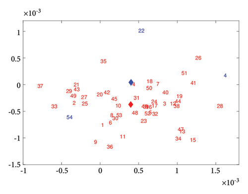
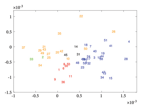
Figure 7 shows the posterior means of the latent positions for each country in 2019. The countries in the upper left are all Asian and Oceanic countries, the countries in the lower middle are all American countries, the countries on the right are all European countries and the countries in the central part are African countries. This result indicates that the trade network is related to geography. African countries have central positions but small radii, indicating that their foreign trade is not well developed, and that they have only established relatively close trade relations with countries with greater influence. China, United States of America, and Germany are located in the central region and have large radii, indicating that these countries have a significant influence on the international trade network, and have close trade relations with many countries.

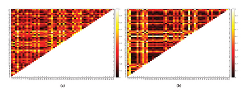
The results indicate that latent positions are related to geographical positions. To further compare latent distances and geographical distances, the article includes a heatmap, as shown in Figure 8. We can see a certain correlation between latent distances and geographical distances, but differences are also evident. The alignment of light and dark columns in the two diagrams exhibits some similarities. However, the right diagram shows distinct black blocks not present in the left one. Moreover, the correlation coefficient between latent distances and geographical distances is 0.4210, suggesting that there is some connection between them, but this connection is not very strong.

To further analyse the latent space, we combined the results of the latent positions, radii, β_IN + β_OUT and η_ijt. Table 7 presents the results related to the maximum and minimum values of η_ijt and ‖x_it − x_jt‖ in 2019. It can be seen that, the latent distance between node 37 and node 4 is the largest. The values of η_ijt between these two nodes are 9.0873 and 8.6938. Although the latent distance is the largest, the radii scale the distance, resulting in η_ijt not being too small. The latent distance between node 46 and node 39 is the smallest. The values of η_ijt between these two countries are 16.0869 and 16.0763, which are very close to the value of β_IN + β_OUT. Furthermore, the maximum value of η_ijt is 16.1580 in 2019. This value is generated from China to the United States. The latent distance between these two countries is small, and both countries have large radii. The minimum value of η_ijt is 4.9970, which is generated from Colombia to Iran. The latent distance between these two countries is large, and both countries have small radii.

Table 7. The maximum and minimum values of ‖x_it − x_jt‖ and η_ijt in 2019.

	Latent distance	Radius of node i	Radius of node j	η_ijt	(i, j)
Maximum of ‖x_it − x_jt‖	0.0024	0.0072	0.0043	9.0873 8.6938	(37, 4)
Minimum of ‖x_it − x_jt‖	1.8115 × 10⁻⁵	0.0067	0.0021	16.0869 16.0763	(46, 39)
Maximum of η_ijt	1.7662 × 10⁻⁴	0.2074	0.1593	16.1580	(10, 53)
Minimum of η_ijt	0.0020	0.0025	0.0037	4.9970	(11, 22)

Note: Numbers represent the country’s serial number.

In addition, we can derive the importance of nodes in the international trade network, as shown in Table 8. A node is considered to be located in the central part of the latent space if the distance between its latent position vector in 2019 and the mean vector of all nodes’ latent positions is smaller than the average of all such distances. Specifically, let , , , if , then country i is located in the central part of the latent space. Where x_i denotes the latent position vector of country i in 2019. It can be seen that countries located in the central part of the latent space and having larger radii include China, France, Germany, India, Italy, the Netherlands, the United Kingdom, and the United States. These countries have significant importance in the international trade network, and all have large trade volumes. Countries located on the periphery of the latent space and having large radii include Japan, Republic of Korea, Russian Federation, and Viet Nam. Despite having a large radiation radius, these countries have a limited range of main trade products. Trade protectionist policies and other factors have imposed certain restrictions on their trade, leading to a less prominent importance of these countries compared to the previously mentioned 8 countries in international trade. There are 22 countries located in the central part of the latent space and having small radii. These countries have a limited number of trade partners, highly concentrated trade volumes, and their importance in the international trade network is not significant. There are 20 countries located on the periphery of the latent space and having small radii. Compared to the countries in the previous three scenarios, these 20 countries are less active in the international trade network, and have relatively small trade volumes.

Table 8. Results of node importance.

Characteristics	Countries
With a radius greater than 0.01, and located in the central part of the latent space	10, 16, 17, 20, 24, 32, 52, 53
With a radius greater than 0.01, and located on the periphery of the latent space	25, 27, 41, 54
With a radius smaller than 0.01, and located in the central part of the latent space	1, 3, 5, 6, 7, 8, 12, 14, 18, 19, 23, 30, 31, 38, 39, 40, 42, 44, 45, 46, 48, 50
With a radius smaller than 0.01, and located on the periphery of the latent space	2, 4, 9, 11, 13, 15, 21, 22, 26, 28, 29, 33, 34, 35, 36, 37, 43, 47, 49, 51

Note: Numbers represent the country’s serial number.

6. Summary

In this paper, we propose a DLS-PC, a novel model that combines a DLS model with a random block model. This model embodies the common reciprocity, transitivity and clustering of network data, reflects global and local characteristics, and can be used for visual analysis. The model is estimated using the Bayesian method based on MCMC, and a Procrustes transformation is performed to reorient the sampled trajectories of the latent positions. A purity-based relabelling algorithm is proposed to resolve label switching. Finally, this paper conducts an empirical analysis of the international trade network.

The results show that the intensities of international trade are related to the geographical location of the countries. The intensity of international trade is mostly determined by the exporting countries. China, the United States of America, and Germany have wider influence ranges in the network. In the trade network of 54 countries, the countries are divided into two classes, which are primarily based on the variance of the latent positions. The three countries with the greatest variance of latent positions are grouped together. The latent positions of the 54 countries did not show significant differences between 2010 and 2019.

Conflicts of Interest

The author declares no conflicts of interest.

Funding

No funding was received for this research.

Appendix A: Country Names for Empirical Research

Table A1 lists the countries and their serial numbers. A total of 54 countries are included in this study.

Table A1. Serial numbers and countries.

Serial number	Country
1	Argentina
2	Australia
3	Austria
4	Belarus
5	Belgium
6	Brazil
7	Bulgaria
8	Canada
9	Chile
10	China
11	Colombia
12	Czech Republic
13	Denmark
14	Egypt
15	Finland
16	France
17	Germany
18	Greece
19	Hungary
20	India
21	Indonesia
22	Iran, Islamic Republic of
23	Ireland
24	Italy
25	Japan
26	Kazakhstan
27	Korea, Republic of
28	Lithuania
29	Malaysia
30	Mexico
31	Morocco
32	Netherlands
33	New Zealand
34	Norway
35	Pakistan
36	Peru
37	Philippines
38	Poland
39	Portugal
40	Romania
41	Russian Federation
42	Saudi Arabia
43	Singapore
44	Slovakia
45	South Africa
46	Spain
47	Sweden
48	Switzerland
49	Thailand
50	Türkiye
51	Ukraine
52	United Kingdom
53	United States of America
54	Viet Nam

Open Research

Data Availability Statement

The data that support the findings of this study are available in International Trade Centre at https://www.intracen.org. These data were derived from the following resources available in the public domain: TRADE MAP (https://www.trademap.org).

References

1 Zhu X., Pan R., Li G., Liu Y., and Wang H., Network Vector Autoregression, Annals of Statistics. (2017) 45, no. 3, 1096–1123, https://doi.org/10.1214/16-aos1476, 2-s2.0-85020646438.
10.1214/16-aos1476
Web of Science® Google Scholar
2 Ward M., Ahlquist J., and Rozenas A., Gravity’s Rainbow: A Dynamic Latent Space Model for the World Trade Network, Network Science. (2013) 1, no. 1, 95–118, https://doi.org/10.1017/nws.2013.1, 2-s2.0-84888059040.
10.1017/nws.2013.1
Google Scholar
3 Hunter D., Krivitsky P., and Schweinberger M., Computational Statistical Methods for Social Network Models, Journal of Computational & Graphical Statistics. (2012) 21, no. 4, 856–882, https://doi.org/10.1080/10618600.2012.732921, 2-s2.0-84898866090.
10.1080/10618600.2012.732921
PubMed Web of Science® Google Scholar
4 Kim B., Lee K., Xue L., and Niu X., A Review of Dynamic Network Models with Latent Variables, Statistics Surveys. (2018) 12, 105–135, https://doi.org/10.1214/18-ss121, 2-s2.0-85057817544.
10.1214/18-ss121
PubMed Web of Science® Google Scholar
5 Salter-Townshend M., White A., Gollini I., and Murphy T., Review of Statistical Network Analysis: Models, Algorithms, and Software, Statistical Analysis and Data Mining: The ASA Data Science Journal. (2012) 5, no. 4, 243–264, https://doi.org/10.1002/sam.11146, 2-s2.0-84864057385.
10.1002/sam.11146
Google Scholar
6 Lusher D., Koskinen J., and Robins G., Exponential Random Graph Models for Social Networks, Theory, Methods, and Applications, 2013, Cambridge University Press.
Google Scholar
7 von Luxburg U., A Tutorial on Spectral Clustering, Statistics and Computing. (2007) 17, no. 4, 395–416, https://doi.org/10.1007/s11222-007-9033-z, 2-s2.0-34548583274.
10.1007/s11222-007-9033-z
Web of Science® Google Scholar
8 Lorrain F. and White H., Structural Equivalence of Individuals in Social Networks, Journal of Mathematical Sociology. (1971) 1, no. 1, 49–80, https://doi.org/10.1080/0022250x.1971.9989788, 2-s2.0-0001964443.
10.1080/0022250x.1971.9989788
Google Scholar
9 Holland P., Laskey K., and Leinhardt S., Stochastic Blockmodels: First Steps, Social Networks. (1983) 5, no. 2, 109–137, https://doi.org/10.1016/0378-8733(83)90021-7, 2-s2.0-0012864758.
10.1016/0378-8733(83)90021-7
Web of Science® Google Scholar
10 Snijders T. and Nowicki K., Estimation and Prediction for Stochastic Blockmodels for Graphs With Latent Block Structure, Journal of Classification. (1997) 14, no. 1, 75–100, https://doi.org/10.1007/s003579900004, 2-s2.0-0031495186.
10.1007/s003579900004
Web of Science® Google Scholar
11 Nowicki K. and Snijders T., Estimation and Prediction for Stochastic Blockstructures, Journal of the American Statistical Association. (2001) 96, no. 455, 1077–1087, https://doi.org/10.1198/016214501753208735, 2-s2.0-0442296603.
10.1198/016214501753208735
Web of Science® Google Scholar
12 Matias C. and Miele V., Statistical Clustering of Temporal Networks Through a Dynamic Stochastic Block Model, Journal of the Royal Statistical Society—Series B: Statistical Methodology. (2017) 79, no. 4, 1119–1141, https://doi.org/10.1111/rssb.12200, 2-s2.0-84994519255.
10.1111/rssb.12200
Web of Science® Google Scholar
13 Hoff P., Raftery A., and Handcock M., Latent Space Approaches to Social Network Analysis, Journal of the American Statistical Association. (2002) 97, no. 460, 1090–1098, https://doi.org/10.1198/016214502388618906, 2-s2.0-0036967824.
10.1198/016214502388618906
Web of Science® Google Scholar
14 Sewell D. and Chen Y., Latent Space Models for Dynamic Networks, Journal of the American Statistical Association. (2015) 110, no. 512, 1646–1657, https://doi.org/10.1080/01621459.2014.988214, 2-s2.0-84939850392.
10.1080/01621459.2014.988214
CAS Web of Science® Google Scholar
15 Lyu Z., Xia D., and Zhang Y., Latent Space Model for Higher-Order Networks and Generalized Tensor Decomposition, Journal of Computational & Graphical Statistics. (2023) 32, no. 4, 1320–1336, https://doi.org/10.1080/10618600.2022.2164289.
10.1080/10618600.2022.2164289
Web of Science® Google Scholar
16 Matias C. and Robin S., Modeling Heterogeneity in Random Graphs Through Latent Space Models: A Selective Review, ESAIM: Proceedings and surveys. (2014) 47, 55–74, https://doi.org/10.1051/proc/201447004.
10.1051/proc/201447004
Google Scholar
17 Zhang X., Xu G., and Zhu J., Joint Latent Space Models for Network Data With High-Dimensional Node Variables, Biometrika. (2022) 109, no. 3, 707–720, https://doi.org/10.1093/biomet/asab063.
10.1093/biomet/asab063
Web of Science® Google Scholar
18 Handcock M., Raftery A., and Tantrum J., Model-Based Clustering for Social Networks, Journal of the Royal Statistical Society—Series A: Statistics in Society. (2007) 170, no. 2, 301–354, https://doi.org/10.1111/j.1467-985x.2007.00471.x, 2-s2.0-34247111980.
10.1111/j.1467-985x.2007.00471.x
Web of Science® Google Scholar
19 Sewell D. and Chen Y., Latent Space Approaches to Community Detection in Dynamic Networks, Bayesian Analysis. (2017) 12, no. 2, 351–377, https://doi.org/10.1214/16-ba1000, 2-s2.0-85019094779.
10.1214/16-ba1000
Web of Science® Google Scholar
20 Casarin R. and Peruzzi A., A Dynamic Latent-Space Model for Asset Clustering, Studies in Nonlinear Dynamics & Econometrics. (2024) 28, no. 2, 379–402, https://doi.org/10.1515/snde-2022-0111.
10.1515/snde-2022-0111
Web of Science® Google Scholar
21 Daniel Loyal J. and Chen Y., A Bayesian Nonparametric Latent Space Approach to Modeling Evolving Communities in Dynamic Networks, Bayesian Analysis. (2023) 18, no. 1, 49–77, https://doi.org/10.1214/21-ba1300.
10.1214/21-ba1300
Google Scholar
22 Frank O. and Harary F., Cluster Inference by Using Transitivity Indices in Empirical Graphs, Journal of the American Statistical Association. (1982) 77, no. 380, 835–840, https://doi.org/10.1080/01621459.1982.10477895, 2-s2.0-0010830161.
10.1080/01621459.1982.10477895
Web of Science® Google Scholar
23 Wasserman S. and Faust K., Social Network Analysis: Methods and Applications, 1994, Cambridge University Press.
10.1017/CBO9780511815478
Google Scholar
24 Sewell D. and Chen Y., Latent Space Models for Dynamic Networks With Weighted Edges, Social Networks. (2016) 44, 105–116, https://doi.org/10.1016/j.socnet.2015.07.005, 2-s2.0-84939864319.
10.1016/j.socnet.2015.07.005
Web of Science® Google Scholar
25 Sarkar P. and Moore A., Dynamic Social Network Analysis Using Latent Space Models, ACM SIGKDD Explorations Newsletter. (2005) 7, no. 2, 31–40, https://doi.org/10.1145/1117454.1117459.
10.1145/1117454.1117459
Google Scholar
26 Geweke J. and Tanizaki H., Bayesian Estimation of State-Space Models Using the Metropolis-Hastings Algorithm Within Gibbs Sampling, Computational Statistics & Data Analysis. (2001) 37, no. 2, 151–170, https://doi.org/10.1016/s0167-9473(01)00009-3, 2-s2.0-0035964376.
10.1016/s0167-9473(01)00009-3
Web of Science® Google Scholar
27 Roberts G. and Rosenthal J., Examples of Adaptive MCMC, Journal of Computational & Graphical Statistics. (2009) 18, no. 2, 349–367, https://doi.org/10.1198/jcgs.2009.06134, 2-s2.0-70349290724.
10.1198/jcgs.2009.06134
Web of Science® Google Scholar
28 Schmon S. and Gagnon P., Optimal Scaling of Random Walk Metropolis Algorithms Using Bayesian Large-Sample Asymptotics, Statistics and Computing. (2022) 32, no. 2, https://doi.org/10.1007/s11222-022-10080-8.
10.1007/s11222-022-10080-8
PubMed Web of Science® Google Scholar
29 Borg I. and Groenen P., Modern Multidimensional Scaling: Theory and Applications, 2005, 2nd edition, Springer Science+Business Media, Inc, New York.
Google Scholar
30 Jasra A., Holmes C., and Stephens D., Markov Chain Monte Carlo Methods and the Label Switching Problem in Bayesian Mixture Modeling, Statistical Science. (2005) 20, no. 1, 50–67, https://doi.org/10.1214/088342305000000016, 2-s2.0-22544479764.
10.1214/088342305000000016
Web of Science® Google Scholar
31 Frühwirth-Schnatter S., Markov Chain Monte Carlo Estimation of Classical and Dynamic Switching and Mixture Models, Journal of the American Statistical Association. (2001) 96, no. 453, 194–209, https://doi.org/10.1198/016214501750333063, 2-s2.0-1842815959.
10.1198/016214501750333063
Web of Science® Google Scholar
32 Manning C., Raghavan P., and Schütze H., Introduction to Information Retrieval, 2008, Cambridge University Press.
10.1017/CBO9780511809071
Google Scholar
33 Oh M. and Raftery A., Bayesian Multidimensional Scaling and Choice of Dimension, Journal of the American Statistical Association. (2001) 96, no. 455, 1031–1044, https://doi.org/10.1198/016214501753208690, 2-s2.0-0442280664.
10.1198/016214501753208690
Web of Science® Google Scholar
34 Raftery A., Bayesian Model Selection in Social Research, Sociological Methodology. (1995) 25, 111–163, https://doi.org/10.2307/271063.
10.2307/271063
Web of Science® Google Scholar
35 Smith M., Gorgoni S., and Cronin B., International Production and Trade in a High-Tech Industry: A Multilevel Network Analysis, Social Networks. (2019) 59, 50–60, https://doi.org/10.1016/j.socnet.2019.05.003, 2-s2.0-85066432501.
10.1016/j.socnet.2019.05.003
Web of Science® Google Scholar
36 Wu G., Feng L., Peres M., and Dan J., Do Self-Organization and Relational Embeddedness Influence Free Trade Agreements Network Formation? Evidence From an Exponential Random Graph Model, Journal of International Trade & Economic Development. (2020) 29, no. 8, 995–1017, https://doi.org/10.1080/09638199.2020.1784254.
10.1080/09638199.2020.1784254
Web of Science® Google Scholar
37 Zhou M., Wu G., and Xu H., Structure and Formation of Top Networks in International Trade, 2001-2010, Social Networks. (2016) 44, 9–21, https://doi.org/10.1016/j.socnet.2015.07.006, 2-s2.0-84939602752.
10.1016/j.socnet.2015.07.006
Web of Science® Google Scholar
38 Goldstein J., Rivers D., and Tomz M., Institutions in International Relations: Understanding the Effects of the GATT and the WTO on World Trade, International Organization. (2007) 61, no. 1, 37–67, https://doi.org/10.1017/s0020818307070014, 2-s2.0-33947376061.
10.1017/s0020818307070014
Web of Science® Google Scholar

All articles

Dynamic Latent Space Model With Position Clusters and Its Application in International Trade Network

Abstract

1. Introduction

2. DLS-PC

3. Estimation