This work examines a discrete prey–predator model using the fractional derivative. The conditions for the existence and stability of the fixed points in the model are identified. The analysis is centered on exploring various bifurcations at the positive fixed point to understand their ecological implications. Using bifurcation theory, bifurcations related to period doubling, Neimark–Sacker, and strong resonances are studied. Lastly, the analytical results are confirmed through numerical simulations using the MATLAB package MatContM, and a controller is applied to relieve the extreme instability within the system.

1. Introduction

The interaction between prey and predator has always been a crucial focus in ecological modeling. The Lotka–Volterra model, recognized as the fundamental prey–predator model, was developed separately by Lotka in 1925 [1] and Volterra in 1926 [2]. It described the dynamics of prey and predator species in terms of differential equations, capturing the essential processes of birth, death, predation, and competition. The Lotka–Volterra model assumes a linear relationship between the rate of prey consumption by predators and the prey population density. This assumption might hold at low prey concentrations, but it is impractical in high prey densities, where predators are few.

In this context, a more general form of a prey–predator model [1, 2] is examined as follows:

()

where x and y represent the population densities of the prey and predator at time t, respectively. The per capita growth rate of the prey is given by g(x), and the predator’s intrinsic death rate is denoted by d. The prey–predator interaction is captured by p(x, y), which is the functional response function. Ecologically, the functional response pertains to the consumption capability of a consumer, which is determined by the density of available food. The functional response of a predator characterizes the correlation between its consumption rate and the abundance or density of the prey population [3, 4]. Different species show various rates of growth in the prey–predator scenario. The evolution of prey populations is analyzed using the logistic map as follows:

()

where r denotes the prey’s intrinsic growth rate. The functional response in the Lotka–Volterra model is represented as follows: p(x, y) ≡ p(x) = αx, α > 0, and then predator–prey model (1) can be written as

()

where a = a₀α and b = b₀α. After their seminal work, researchers introduced more realistic prey–predator models that include Holling type [3, 5, 6], Ivlev [7], and ratio-dependent functional responses [8–10]. Ecologists have also considered various ecological effects, such as the Allee effect [11], fear effect [12], harvesting [13], and shelter effect, to enhance the understanding of prey–predator interactions.

Recently, differential equations with fractional-order derivatives have garnered significant interest from researchers due to their ability to accurately describe a variety of nonlinear phenomena [14]. These equations have been applied across numerous fields of science and engineering, such as biology [15], medicine [16], fluid mechanics, and physics [17, 18]. Fractional-order derivatives are particularly effective in capturing complex behaviors, long-term population fluctuations, and irregular oscillations in ecological systems [19, 20]. This also accounts for memory effects, where the current state of a population is influenced by its past states, a concept highly relevant in ecological studies [21]. As a result, fractional-order derivatives have been successfully applied in mathematical biology [22–24]. Numerous researchers have explored fractional-order continuous prey–predator models [25–27]. Different approaches to the stability of differential equations can be found in [28, 29].

In the model described by equation (1), the growth rates of both prey and predator are based only on current conditions. However, long-term memory is also a crucial factor influencing population growth rates. Taking into account memory effects, many researchers have employed fractional derivatives to develop fractional differential equations [21]. Various definitions of fractional derivatives exist in the literature [30], with the Riemann–Liouville and Caputo derivatives being among the most widely used in the field of fractional-order nonlinear dynamical systems. Unlike integer-order derivatives, fractional derivatives require a broader range of initial conditions that can be challenging to establish. For instance, the Riemann–Liouville derivative requires initial conditions in terms of fractional derivatives, which can complicate the formulation of boundary conditions for certain problems. The Caputo derivative offers advantages over other fractional-order derivatives, primarily because it only needs initial conditions in the form of integer-order derivatives, making it better suited for the mathematical modeling of many real-world problems. In addition, the fractional-order operator allows for greater flexibility in various physical and biological models, enabling a deeper analysis of their significant dynamic behaviors [30, 31]. This research is motivated by the need for a deeper understanding of prey–predator models incorporating the effect of memory. Therefore, the Caputo fractional–order derivative is applied in the model (3), making it more applicable to modeling and analysis.

Definition 1 (see [21], [30].)Caputo fractional derivative of order of the function , t ≥ t₀ is defined by

()

where Γ(·) denotes the Gamma function. Particularly, when 0 < α < 1,

()

Using the fractional-order Caputo-type derivatives, model (3) takes the following form:

()

In model (6), the Caputo fractional derivative allows for the incorporation of memory effects and hereditary properties in the modeling process, making it particularly suitable for biological systems where the current state depends on the historical states.

In ecology, certain species, such as gypsy moths and many other insects, have populations where generations do not overlap. In these cases, using a discrete-time prey–predator model is often more suitable. Over the past few decades, there has been an increasing interest in researching discrete-time dynamical systems [32–34]. It has also been demonstrated that discrete models can display more complex dynamical behaviors. Codimension-1 bifurcations in discrete prey–predator models with various functional responses have been explored in these studies. Rana [35] examined the dynamics of a discrete-time prey–predator system of Leslie-type and demonstrated that the system undergoes a period-doubling (PD) bifurcation and a Neimark–Sacker (NS) bifurcation. An analysis of codimension-1 bifurcation of the discrete prey–predator model (7) was conducted by Liu and Xiao [36], utilizing the forward Euler scheme in model (3).

()

Higher codimension bifurcations have gained importance in discrete-time models throughout the past 10 years due to their more fascinating dynamics. Codimension-2 bifurcations have received significant attention due to the presence of resonance bifurcations among them. Kuznetsov, Kuznetsov, and Kuznetsov [37] proposed the codimension-2 resonance bifurcation theory for discrete maps for the first time. One can use the crucial normal form coefficient hypothesis to find resonance bifurcations such as 1:2, 1:3, and 1:4. Zhang, Xu, and Liao [38] investigated the codimension-2 bifurcations and bifurcation controls of a discrete predatory system with weak Allee effect on prey. Sharma et al. [39] explored codimension-1 and codimension-2 bifurcations including multiple and generic bifurcations in the discrete model using the critical normal form theorem and bifurcation theory. Li, Eskandari, and Avazzadeh [40] introduced a two-dimensional discrete-time prey–predator model and identified bifurcation scenarios based on critical coefficients. In addition to these studies, recent research has also investigated codimension-2 bifurcations in discrete-time prey–predator models [41, 42]. The resonance bifurcations of model (7) and its dynamic behavior were investigated by Ma and Duan [42], using the normal form method and the theory of approximation by a flow.

Recently, Din [43] examined the qualitative dynamics of a discrete fractional-order Brusselator model, utilizing normal form theory and the center manifold theorem (CMT) to demonstrate the occurrence of both codimension-1 and codimension-2 bifurcations. Discrete-time prey–predator models using fractional-order derivatives, however, have received little attention [44, 45]. George et al. [46] investigated stability, PD bifurcation, and sensitive dependence to initial conditions in a discrete fractional-order prey–predator model with harvesting. Uddin et al. [13] explored a discrete prey–predator model, including harvesting on the predator population, using Caputo fractional derivative. These studies emphasized analyzing stability and one-parameter bifurcations, such as PD and NS bifurcations using the center manifold and bifurcation theory. However, the current study focuses on two-parameter bifurcations to provide a deeper understanding of the system’s dynamics.

The discrete fractional-order prey–predator model (6) by performing the discretization technique for a fractional-order system as described in [47] is derived as

()

where x_n and y_n are densities of the prey and predator population in a discrete-time system. This study clarifies that model (8) does not introduce an entirely new model in the literature but instead extends the model in [36, 42] by incorporating the memory effects through the use of Caputo fractional derivatives. While the studies in [36, 42] examined similar models utilizing the forward Euler scheme, they do not account for historical effects in species interactions. Integrating the Caputo fractional derivative into discrete prey–predator models enhances the ability to capture memory-dependent dynamics, providing a more comprehensive view of prey–predator interactions and potentially leading to better management and conservation strategies. This approach can lead to rich and complex dynamics, including stability, oscillatory behavior, and resilience of populations in changing ecological conditions. The following few points highlight the special contributions and novelty of this study:

•
The importance of memory effects into species interactions developed by discrete fractional-order model (8), defined in the Caputo sense, provides a powerful tool for understanding complex ecological dynamics.
•
To examine the presence and topological classification of fixed points.
•
The exploration of potential codimension-1 and codimension-2 bifurcations of model (8) using critical normal form theory.
•
To validate the theoretical findings, an efficient numerical method is employed. The results demonstrate the effectiveness of the proposed model in offering new insights into the dynamic behavior and influence of control parameters.
•
A feedback control strategy is implemented to manage the model’s (8) unpredictability.

This paper’s subsequent sections are formatted as follows. Local stability is examined in Section 2. Section 3 covers bifurcation analysis, including codimension-1 and codimension-2 bifurcations. Numerical simulations using MatContM are conducted to validate the analytical findings, as presented in Section 4. Techniques for controlling chaos are covered in Section 5. Section 6 presents the ecological implications and discussion. A brief conclusion is outlined in Section 7.

2. The Fixed Points: Existence and Stability

In the region

, let (x^f, y^f) be any fixed point of (8) such that

()

The fixed points are as follows:

i.
E₀ = (0, 0)
ii.
E₁ = (1, 0)
iii.
E_f = (d/b, r(b − d)/ab)

The fixed points E₀ and E₁ are the trivial and axial points, respectively, which always exist. For the interior fixed point E_f, b > d is the existence condition.

Model (8) examined at any location (x, y) yields the following Jacobian matrix:

()

and we have

()

One can see Table 1 for the stability conditions of trivial and axial fixed points of model (8) using Jury’s criterion [48].

Table 1. Topological properties of model (5) at fixed points E_i(i = 0, 1).

Fixed points	Eigenvalues	Dynamic behavior	Relative parametric requirements
E₀	μ₁ = 1 − dρ^α/(Γ(α + 1)),	Source	d > 2ρ^−αΓ(α + 1);
	μ₂ = (rρ^α/(Γ(α + 1))) + 1	Saddle	d < 2ρ^−αΓ(α + 1);
	μ₂ = (rρ^α/(Γ(α + 1))) + 1	Nonhyperbolic	d = 2ρ^−αΓ(α + 1) (with PD bifurcation).

E₁	μ₁ = (ρ^α(b − d)/(Γ(α + 1))) + 1,	Source	d > ρ^−α(2Γ(α + 1) + bρ^α), d < b, r > 2ρ^−αΓ(α + 1);
	μ₂ = 1 − (rρ^α/(Γ(α + 1)))	Sink	b < d < ρ^−α(2Γ(α + 1) + bρ^α), r < 2ρ^−αΓ(α + 1);
		Nonhyperbolic	d = ρ^−α(2Γ(α + 1) + bρ^α), d ≠ b, r ≠ 2ρ^−αΓ(α + 1) or r = 2ρ^−αΓ(α + 1), d ≠ b, d ≠ ρ^−α(2Γ(α + 1) + bρ^α) (with PD bifurcation), d ≠ ρ^−α(2Γ(α + 1) + bρ^α), d = b, r ≠ 2ρ^−αΓ(α + 1) (with fold bifurcation);
		Saddle	Otherwise.

The characteristic equation for ℷ(E_f) can be expressed as

()

Therefore, the eigenvalues of ℷ(E_i) are

where

, and we have

()

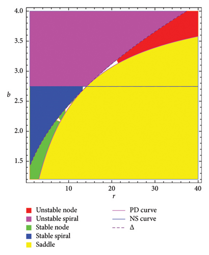
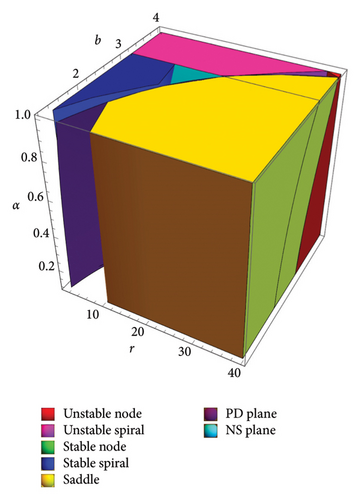
The following statement gives the sufficient and necessary criteria for the local stability of the interior fixed point of model (8) according to [48]. For more information, we refer to Figure 1. The region for the stability (topological classification) of fixed point E_f in two-parameter (r, b)-space is presented in Figure 1(a). The time scale is crucial when interpreting stability regions, especially for identifying the behavior of dynamical systems over time. It describes how quickly a system evolves toward stability or instability near a fixed point. The PD curve represents a boundary where periodic solutions double their period, eventually leading to chaotic dynamics. The NS curve shows where fixed points lose stability through a Hopf bifurcation, leading to oscillations. Stability regions are labeled where different system dynamics arise (color:system dynamics at a fixed point). Red: unstable node, pink: unstable spiral, green: stable node, blue: stable spiral, and yellow: saddle. The dashed line divides the space to identify the nature of multipliers: above the dashed line, the multipliers are real, while on the other side, the multipliers are complex. Therefore, below the NS curve, the solutions are stable (e.g., spirals or nodes), whereas above the NS curve or PD curve, instability arises, potentially leading to chaotic or oscillatory behavior. To illustrate the effect of memory on the dynamics of model (8), a three-dimensional Figure 1(b) is depicted.

Details are in the caption following the image — **Figure 1 (a)**
Open in figure viewer PowerPoint

Stability regions of fixed point E_f for model (5) in (a)(r, b)-space with α = 0.75, ρ = 0.5, d = 1.2, a = 1.5 and (b)(r, b, α)-space.

Proposition 1. When b > d, the interior fixed point E_f is

•
sink if
- 1.
  Δ ≥ 0 and b > drρ^α(2Γ(α + 1) + dρ^α)/(4Γ(α + 1)² + drρ^2α)
- 2.
  Δ < 0 and b < ρ^−αΓ(α + 1) + d
•
source if
- 1.
  Δ ≥ 0 and b < drρ^α(2Γ(α + 1) + dρ^α)/(4Γ(α + 1)² + drρ^2α)
- 2.
  Δ < 0 and b > ρ^−αΓ(α + 1) + d
•
nonhyperbolic if
- 1.
  Δ ≥ 0 and b = drρ^α(2Γ(α + 1) + dρ^α)/(4Γ(α + 1)² + drρ^2α)
- 2.
  Δ < 0 and b = ρ^−αΓ(α + 1) + d
•
saddle for any other parameter values outside of the ones listed above.

3. Bifurcation Analysis

It is possible to rewrite model (8) as a map as follows:

()

where μ = (ρ, α, r, a, b, d).

Let

, then the fixed points (x^f, y^f) of the system are shifted to the origin, and the system emerges as

()

One way to express map (14) is

()

where the symmetric multilinear vector functions of

are represented by B(x, y) and C(x, y). The following is a description of these functions:

()

and

3.1. One-Parameter Bifurcations at Fixed Points

A dynamical system bifurcates when different parameters cause a qualitative shift in the dynamics of the system. Its codimension is the number of parameters that need to be altered for the occurrence of bifurcation. In equivalent terms, the number of equality conditions characterizing a bifurcation is the codimension. Using bifurcation theory [37, 49], parameter b is considered as a bifurcation parameter, while the remaining parameters are fixed to explore the codimension-1 bifurcations: Transcritical (TC), PD, and NS bifurcations at E_f.

3.1.1. PD Bifurcation

Theorem 1. The critical value d = b for E₁ causes a TC bifurcation in map (14).

Proof 1. The multipliers of

()

are the following:

()

Therefore, on the unit circle, matrix A(E₁, μ_TC) has a simple multiplier of one if . Thus, at critical parameter, F(E₁, μ_TC) can be expressed in the normal form as

()

where

()

As a result,

()

Remark 1. Since β_TC,1 ≠ 0, E₁ develops a TC bifurcation because it is always the fixed point and will never disappear.

Theorem 2. At d = 2ρ^−αΓ(α + 1) + b for E₁, a PD occurs in map (14).

Proof 2. The multipliers of

()

are the following:

()

The 1-D center manifold of map (14) at d = 2ρ^−αΓ(α + 1) + b is taken as

()

On the unit circle, matrix A(E₁, μ_PD) has a simple multiplier of −1 if . Thus, at critical parameter, F(E₁, μ_PD) can be expressed in the normal form as

()

where

()

As a result,

()

Remark 2. As long as the PD is generic, β_PD,1 ≠ 0. When β_PD,1 > 0, the PD displays supercritical behavior; if β_PD,1 < 0, then subcritical behavior is displayed. It is evident from a biological perspective that both species can live together.

Theorem 3. At b = drρ^α(2Γ(α + 1) + dρ^α)/(4Γ(α + 1)² + drρ^2α) for E_f, a PD takes place in map (14).

Proof 3. The multipliers of

()

are the following:

()

The 1-D center manifold of map (14) at b = drρ^α(2Γ(α + 1) + dρ^α)/(4Γ(α + 1)² + drρ^2α) is taken as

()

On the unit circle, matrix A(E_f, μ_PD) has a simple multiplier of −1 if . Thus, at critical parameter, F(E_f, μ_PD) can be expressed in the normal form as

()

where

()

As a result,

()

where

()

Remark 3. As long as the PD is generic, β_PD,f ≠ 0. When β_PD,f > 0, the PD displays supercritical behavior; if β_PD,f < 0, then subcritical behavior is displayed. It is evident from a biological perspective that both species can live together.

3.1.2. NS Bifurcation

Theorem 4. At b = ρ^−αΓ(α + 1) + d, a NS bifurcation takes place for E_f.

Proof 4. The multipliers of

()

are the following:

()

The 1-D center manifold of map (8) at r = (2ab − 2a − b² + 2b)/b is taken as

()

If , matrix A(E_f, μ_NS) has a pair of conjugate multipliers approaching the unit circle. So, F(E_f, μ_NS) can be expressed in the normal form at a specific parameter value

()

where

()

As a result,

()

where

()

Remark 4. As long as , the NS bifurcation is generic. In the case that α_NS,∗ > 0, the bifurcation is supercritical; if α_NS,∗ < 0, it is subcritical.

3.2. Strong Resonance Bifurcations

Codimension-2 bifurcations [37, 49, 50] near the fixed point E_f are addressed in this section. The bifurcation parameters r and b are considered here.

3.2.1. Resonance 1:2 Bifurcation

Theorem 5. Map (14) exhibits a strong resonance 1:2 bifurcation at the fixed point E_f for r = (4ρ^−2αΓ(α + 1)(Γ(α + 1) + dρ^α))/d and b = ρ^−α(Γ(α + 1) + dρ^α).

Proof 5. The resonance 1:2 bifurcation takes place at the fixed point E_f when the corresponding Jacobian matrix ℷ(E_f) has two multipliers with trace(ℷ(E_f)) = −2, Det(ℷ(E_f)) = 1. It implies that at r = (4ρ^−2αΓ(α + 1)(Γ(α + 1) + dρ^α))/d, b = ρ^−α(Γ(α + 1) + dρ^α), the Jacobian matrix

()

has critical multipliers

. So, it is possible to write

()

where

()

and

()

As a result,

()

So, and can be derived as follows:

()

Remark 5. The nondegeneracy of the resonance 1:2 bifurcation is demonstrated by and . The sign of determines the behavior of a fixed point: if , the bifurcation is supercritical, and if , a NS bifurcation curve emerges. The occurrence of the resonance 1:2 bifurcation is governed by the coefficient .

3.2.2. Resonance 1:3 Bifurcation

Theorem 6. For r = (3ρ^−2αΓ(α + 1)(Γ(α + 1) + dρ^α))/d and b = ρ^−α(Γ(α + 1) + dρ^α), map (14) shows resonance 1:3 bifurcation at the fixed point E_f.

Proof 6. The resonance 1:3 bifurcation arises at fixed point E_f when the corresponding Jacobian matrix ℷ(E_f) has two complex conjugate eigenvalues e(±2πi/3) with trace(ℷ(E_f)) = 1, Det(ℷ(E_f)) = 1. It shows that at r = (3ρ^−2αΓ(α + 1)(Γ(α + 1) + dρ^α))/d, b = ρ^−α(Γ(α + 1) + dρ^α), the Jacobian matrix

()

has critical multipliers

. So,

can be written as

()

where

()

and

()

As a result,

()

So, can be derived as follows:

()

For reducing the complexity, we set α = 0.875, a = 0.94, d = 0.5, and ρ = 0.75 and we obtain .

Remark 6. and indicate that the bifurcation is generic. The stability of an invariant curve with period-3, which bifurcates from the fixed point near the R3 point, is determined by the coefficient .

3.2.3. Resonance 1:4 Bifurcation

Theorem 7. The map (14) shows resonance 1:4 bifurcation at the fixed point E_f for r = (2ρ^−2αΓ(α + 1)(Γ(α + 1) + dρ^α))/d and b = ρ^−α(Γ(α + 1) + dρ^α).

Proof 7. When the associated Jacobian matrix ℷ(E_f) has two complex conjugate multipliers e^±πi/2 with trace(ℷ(E_f)) = 0, Det(ℷ(E_f)) = 1, the resonance 1:4 bifurcation occurs at the fixed point E_f. It implies that at r = (2ρ^−2αΓ(α + 1)(Γ(α + 1) + dρ^α))/d and b = ρ^−α(Γ(α + 1) + dρ^α), the Jacobian matrix

()

has the critical multipliers

. So,

is constrained to the central manifold in the following way:

()

where

()

As a result,

()

So and can be derived as follows:

()

Remark 7. and indicate that the resonance 1:4 bifurcation is generic. The value of determines the bifurcation scenario, indicating that both species remain stable in high periodic cycles up to the fourth order, near certain critical parameter values.

4. Numerical Simulation

This section displays phase portraits, bifurcation diagrams, and Lyapunov exponents obtained from numerical simulations. The analytical results have been verified using the MATLAB toolbox MatContM [51, 52].

4.1. One-Parameter Bifurcations at E_f

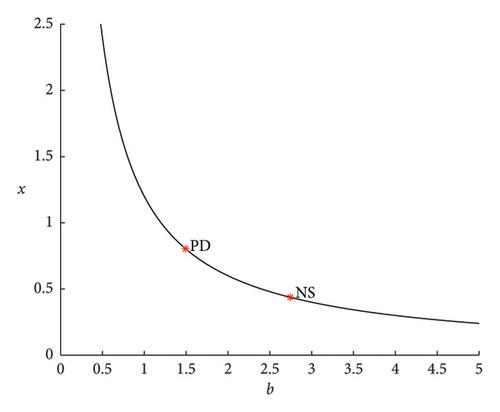
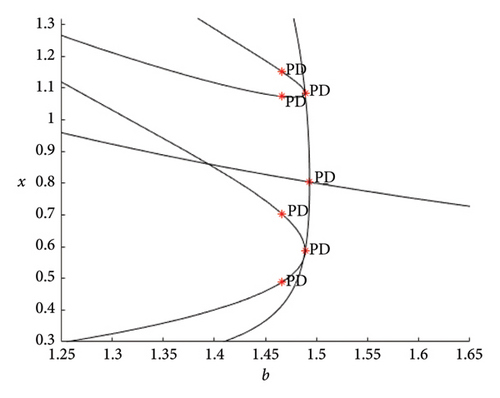
To investigate one-parameter bifurcations, the computation is conducted with fixed parameters α = 0.75, ρ = 0.5, r = 4.25, d = 1.2, a = 1.5 and changing the bifurcation parameter b. First, the PD and NS points are drawn based on the bifurcation parameter b, as shown in Figure 2. By varying parameter b, the one-parameter bifurcations can be generated. MatContM produces the following report.

For PD, x = (0.803610 0.556438 1.493261), normal form coefficient of PD = 1.334768e − 01.
For NS, x = (0.437051 1.595021 2.745673), normal form coefficient of NS = −9.967657e − 01.

As the parameter b varies, the predator–prey model (8) displays significantly more complex behavior. The bifurcation diagram shown in Figure 3 reveals that the model undergoes both PD and NS bifurcations when the parameter b reaches its critical value. Initially, the model exhibits chaotic dynamics for small values of b. However, as b increases, the chaotic behavior suddenly ceases through a PD bifurcation at approximately b ~ 1.49326, leading the model to transition into a stable state. Subsequently, a NS bifurcation occurs at b ~ 2.74567, which then initiates a return to chaotic dynamics. For instance, if ∈[1.25, 1.49326)(b ∈ (1.49326, 1.87867)), eigenvalues of the Jacobian matrix at E_f are real with magnitudes greater than 1 (less than 1), and the fixed point is a saddle (stable node). In contrast, if ∈(1.87867, 2.74567)(b ∈ (2.74567, 3.791]), eigenvalues are complex with magnitudes lower than 1 (higher than 1), and the fixed point is a stable spiral (unstable spiral). The maximum Lyapunov exponents (MLEs) associated with Figure 3(a) are presented in Figure 3(b), confirming the dynamic transition of model (8) from chaotic regimes to stable windows and vice versa. For the eigenvalues λ_i, (i = 1, 2), the time scales are given by τ_i = 1/|ln(λ_i)|. For real eigenvalues, τ_i represents the rate at which perturbations decay or grow and for complex eigenvalues, the real part determines the decay/growth rate, while the imaginary part determines oscillation frequency. The eigenvalues and time scales as a function of bifurcation parameter b are shown in Figures 3(b) and 3(d). These plots show that there is a point where the magnitude of one eigenvalue becomes 1, indicating a change in stability, which corresponds to a bifurcation. On the other hand, as b approaches some key points, the time scales increase noticeably, suggesting that the system slows down near the bifurcation points. As a result, this analysis helps to identify regions in which the dynamics of the system undergoe significant qualitative changes due to bifurcations.

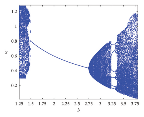
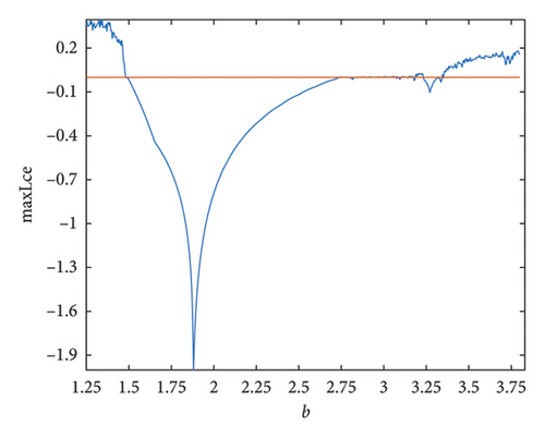
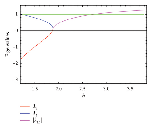
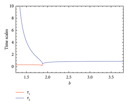
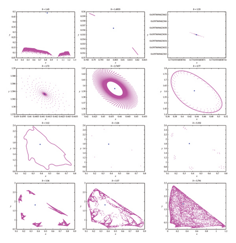
Figure 4 clearly demonstrates that as the parameter b increases, model (8) exhibits alternating behavior between periodic or quasiperiodic states and invariant cycles or chaotic states. For various values of b, the phase portraits of model (8) corresponding to Figure 3, are depicted in Figure 4. These portraits illustrate the stable fixed point for 1.49326 < b < 2.74567, the presence of period-6, and -30 orbits at approximately b ~ 3.26 and b ~ 3.332, respectively. An invariant closed curve occurs at b ~ 2.77 and a breakdown of invariant curve exists for b ~ 3.12 as well as a fully dense chaotic attractor in model (8) at b ~ 3.791. The stability of the bifurcated closed invariant curve suggests that both populations persist in the same environment and their populations may fluctuate but do not become extinct.

Now, the PD point in Figure 2 is selected. At E_PD,∗ = (0.8036100.556438) for b = 1.49326, there is a PD bifurcation with β_PD,∗ = 1.334768e − 01. Figure 5 illustrates how a curve emanating from a PD bifurcation causes the period to double. For b = 2.745673, a NS bifurcation takes place at E_NS,∗ = (0.4370511.595021) with β_NS,∗ = −9.967657e − 01. It concludes that the bifurcation is supercritical since β_NS,∗ < 0. It means that the system transitions to a stable quasiperiodic behavior as the bifurcation parameter is varied, leading to the emergence of a stable invariant torus around the fixed point.

Remark 8. Chaos is often thought to be indicated by positive Lyapunov exponents. The exponents also ensure the emergence of stable periodic windows or stable fixed points within a chaotic region. At b < 1.49326 or b > 2.74567, the greatest Lyapunov exponent is seen in Figure 3(b), confirming the presence of chaos.

4.2. Effects of the Fractional-Order of Model (8) at E_f

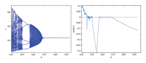
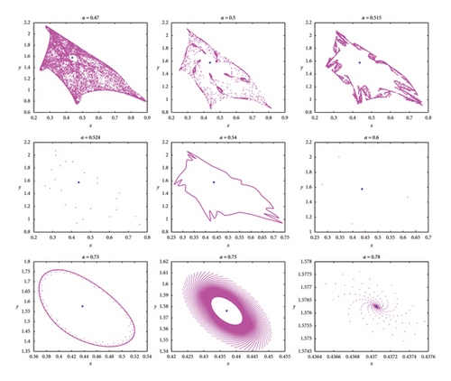
The Caputo fractional derivative allows for the incorporation of memory effects and nonlocal interactions into the model, meaning that the future state of the system depends not only on its current state but also on its past states. When applied to discrete prey–predator models, this fractional derivative can lead to the emergence of chaotic behaviors that enhance understanding of species interactions and their long-term implications. The fractional-order α (where 0 < α < 1) controls the extent of the memory effect. A lower α means a stronger memory effect, leading to a slower response of the system to changes in population. A bifurcation diagram concerning α and the maximum Lyapunov exponents is also depicted in Figure 6. The phase diagrams are illustrated in Figure 7 for various values of α near the NS point. It illustrates that the stability of E_f in the prey–predator model (8) is influenced by the fractional-order α. In this case, the model exhibits stable behavior for α > 0.75, while for others, it becomes unstable or even chaotic.

4.3. Two-Parameters Bifurcations at E_f

To investigate two-parameter bifurcations, the computation is conducted with fixed parameters α = 0.75, ρ = 0.5, d = 1.2, a = 1.5 and varying r and b as bifurcation parameters. By choosing the NS point in Figure 2 and extending the NS curve in two bifurcation parameters r and b, strong resonances of 1:2, 1:3, and 1:4 at fixed point E_f are observed. These resonance bifurcations, identified as R2, R3, and R4, are illustrated in Figure 8. MatContM generates the following report:

Label for R4, x = (0.437051 2.654560 7.073186 2.745673 0.000000) NFC of R4: A = −9.946486e − 01 + 6.335467e − 01 i
Label for R3, x = (0.437051 3.981841 10.609779 2.745673 −0.500000) NFC of R3: Re(c1) = −4.141776e − 01
Label for R2, x = (0.437051 5.309121 14.146372 2.745673 −1.000000) NFC of R2: [c, d] = 8.234240e − 01, −1.134260e + 01

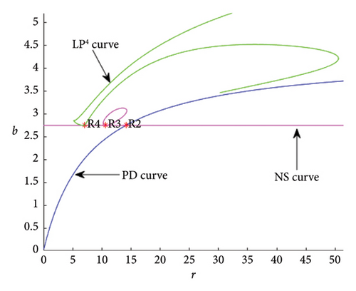
Theorems 5–7 are confirmed by Figure 8. The following key points have been addressed:

•
For r = 7.073186 and b = 2.745673, a resonance 1:4 bifurcation (R4) occurs at E_R4,∗ = (0.114569, 15.927385) with . As Figure 8 illustrates, the R4 point of the model (8) is the source of the fourth iterate’s two-fold curves since .
•
For r = 10.609779 and = 2.745673 , a resonance 1:3 bifurcation (R3) appears at E_R3,∗ = (0.114569, 23.891078) with .
•
For r = 14.146372 and = 2.745673 , a resonance 1:2 bifurcation (R2) exists at E_R2,∗ = (0.114569, 31.854770) with .

Next, we identify the region near the resonance 1:3 by choosing the R3 point in Figure 8. In this region, a closed invariant curve appears to coexist with an unstable fixed point; this curve, known as the NS curve, originates at the R3 point in the third iteration and is also depicted in the same Figure 8. The occurrence of the resonance 1:3 bifurcation at this point leads to the instability of the fixed point E_f. As a result, a neutral saddle bifurcation curve emerges, originating from the R3 point. This Figure 8 describes transitions and bifurcations in a system as parameters r and b change. The green LP curve indicates the onset of saddle-node bifurcation, and its complex looping suggests the coexistence of multiple equilibria. The resonance points (R2, R3, and R4) indicate special parameter values where significant changes occur, such as bifurcation or critical transitions. The system passes through regions where bifurcations (PD or NS) occur. Transitions between stable, unstable, or oscillatory states depend on the relative position of these curves.

The resonance 1:4 bifurcation diagram corresponding to Figure 8 is depicted in Figure 9. It shows that the closed invariant curve becomes less smooth at fixed point E_f and eventually breaks apart as a saddle cycle of period-4 appears. After that, the trajectory changes to orbits with period-4, which then leads to chaotic behavior.

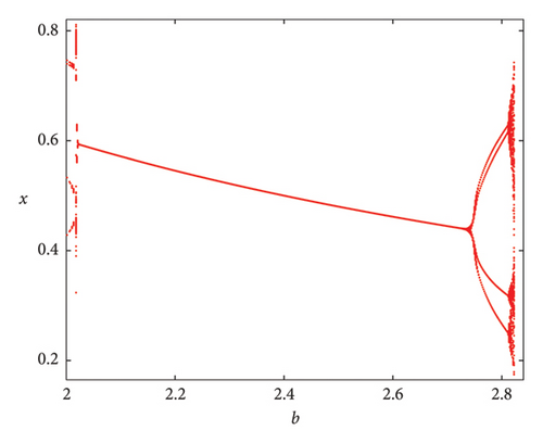
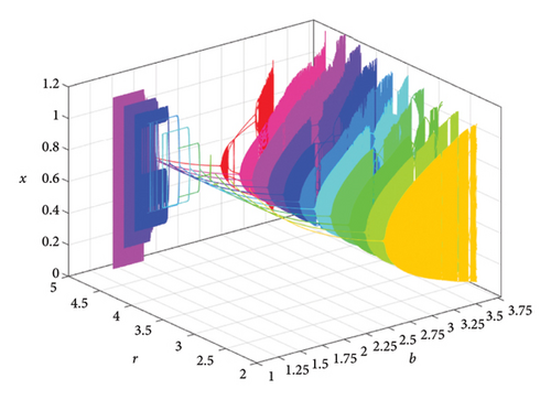
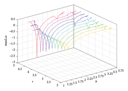
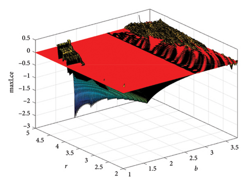
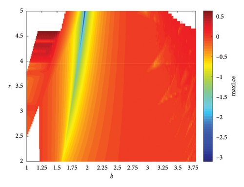
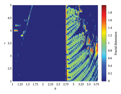
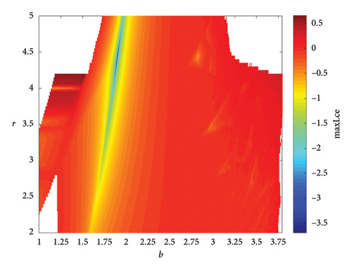
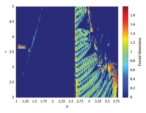
When two additional parameters go over their critical thresholds, the dynamics of model (8) might become more complex. The plots of the bifurcation diagram, 3D MLEs, 3D Lyapunov spectrum and its 2D projection, and 2D projection of 3D fractal dimension for (b, r) ∈ [1.0, 3.8] × [2.0, 5.0], and other parameter values as in Section 4.3 are shown in Figure 10. For α = 0.65, the 2D projection of the 3D Lyapunov spectrum and 3D fractal dimension are presented in Figure 11. These graphics serve as a tool to see how the system dynamics alter qualitatively as parameter values rise. Finding control parameter values for which model (8) dynamics are nonchaotic, periodic, or chaotic is straightforward. Consequently, the system dynamics remarkably shift along the route chaotic–static–chaotic when the values of the control parameters b and r grow, respectively. Furthermore, it illustrates that memory effects (decreasing the α value) influence the emergence of chaotic behavior in the system.

4.4. Comparison of System (7) With Model (8)

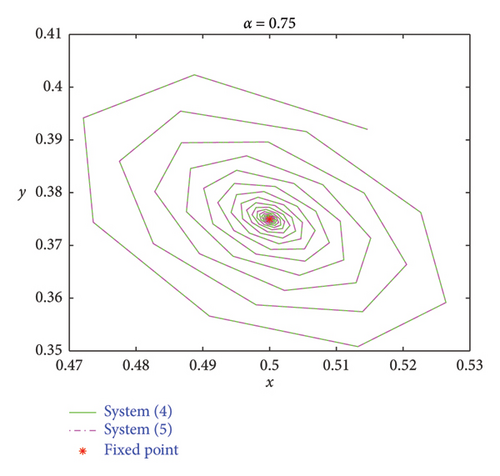
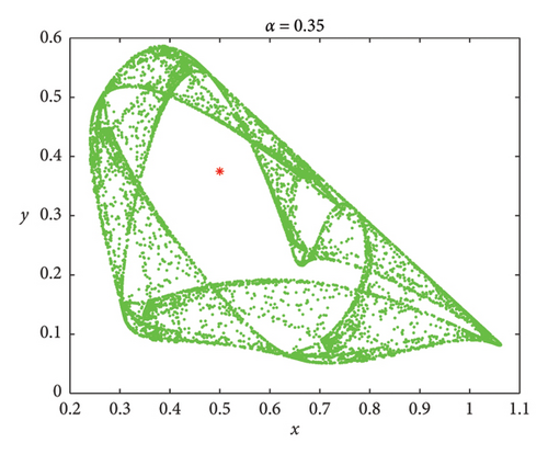
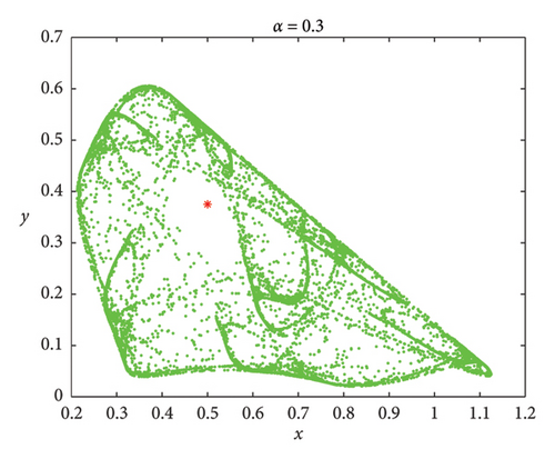
Understanding the impact of memory on prey–predator dynamics, numerical simulations are presented for discrete model (7) to demonstrate that the discrete model (8) exhibits more complex dynamic behaviors. Let the parameters be δ = 0.45, r = 3, a = 4, b = 4, and d = 2 [36]. It follows that both models (7) and (8) admit the same positive fixed point E_f = (1/2, 3/8). We fixed that α = 0.75 and ρ = 0.308137. The phase portraits are depicted in Figure 12(a). However, smaller values of α show that model (8) has much richer dynamic behaviors than model (7) (Figures 12(b) and 12(c)). Therefore, it can be concluded that memory effects in prey–predator dynamics are essential for effective ecosystem management and conservation efforts.

5. Chaos Control

To manage the chaotic behavior observed in model (8), we employ the state feedback control, a technique described in [48]. This approach involves introducing a control force v_n to steer the model towards a stable state.

()

where k₁ and k₂ represent the feedback gain and (x^f, y^f) is a interior fixed point of model (8). The Jacobian matrix of (60) is as follows:

()

The Jacobian matrix’s characteristic equation is

()

where α₁ = −trace(ℷ_c) = (drρ^α/(bΓ(α + 1))) + k₁ − 2, and α₂ = det(ℷ_c) = −(rρ^α(ad + bk₂(d − b))/abΓ(α + 1)) + (drρ^2α(b − d)/bΓ(α + 1)²) − k₁ + 1.

Let μ₁ and μ₂ be the roots of (62). Then,

()

and

()

The marginal stability lines can be obtained by solving the systems of equations μ₁ = ±1 and μ₁μ₂ = 1. These conditions demonstrate that |μ_1,2| < 1. Assume that μ₁μ₂ = 1, then from (64),

()

for μ₁ = 1, and from equations (63) and (64), we obtain

()

Next, for μ₁ = −1, equations (63) and (64) yield that

()

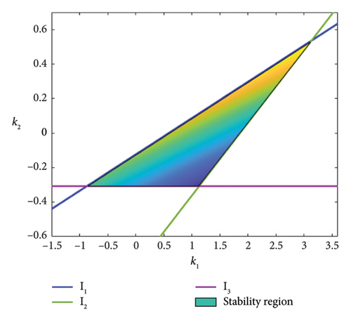
The eigenvalues with a magnitude smaller than 1 are maintained in the triangular region in the (k₁, k₂)-plane, bordered by l₁, l₂, and l₃.

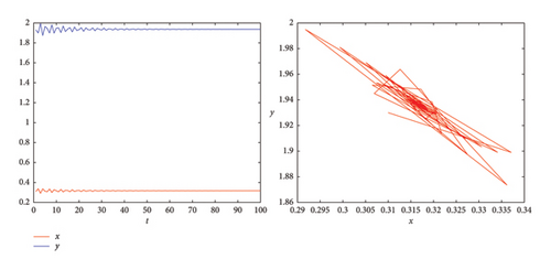
We fix parameter b = 3.791 and the rest as in Section 4. Then, the marginal stability lines are as follows:

()

From the stability region in Figure 13(a), the feedback gains are choosen as k₁ = 2.6 and k₂ = 0.4. The chaotic trajectory is then stabilized as shown in Figure 13(b).

6. Discussion and Ecological Implications

In an ecosystem, there exist different types of interaction among species such as prey–predator, competition, and mutualism. In prey–predator models, prey compete with each other for general resources and predators consume the prey population to survive. Applying Caputo’s fractional derivative to prey–predator models captures important ecological dynamics that classical models often overlook. Incorporating memory effects, nonlocal interactions, and complex oscillatory behaviors provides a more realistic framework for understanding prey–predator systems in real-world contexts. This approach is especially relevant for ecologists and conservationists, as it offers deeper insights into the persistence and sustainability of species interactions and helps predict the long-term impacts of environmental changes on ecosystems.

This study analyzed PD bifurcation, NS bifurcation, and strong resonance, 1 : 2, 1 : 3, and 1 : 4, bifurcations of biologically significant positive fixed point, denoted by E_f, and also analyzed their critical coefficients to investigate the dynamics around the bifurcation point and to assess their nondegeneracy.

At the PD bifurcation point (Figure 2), the eigenvalues associated with the fixed point shift from having negative real parts (indicating a stable fixed point) to positive real parts (indicating an unstable fixed point), or the reverse. In ecological terms, a PD bifurcation (Figure 5) suggests that as a parameter changes, the discrete-time system shifts from a fixed point to a cycle of period-2, indicating that prey and predator populations might coexist under specific conditions. This bifurcation can lead to significant changes in species densities and competition for shared resources, potentially resulting in chaotic dynamics within the population cycles.

The NS bifurcation (Figure 3) involves a qualitative change in the dynamical system. It indicates the onset of a periodic orbit in the system, triggered when a pair of complex conjugate eigenvalues cross the unit circle at the NS bifurcation point. The NS bifurcation marks a transition from a stable fixed point to a stable limit cycle, leading to fluctuations in population size.

The occurrence of strong resonance bifurcation can impact the stability of an ecosystem to a great extent as it can severely fluctuate population size. When R2 bifurcation (Figure 8) occurs at a fixed point, it indicates that NS, heteroclinic, and pitchfork bifurcations could happen in the neighborhood of the fixed point. Chaotic behavior and the formation of new stable orbits might result from R3 bifurcation. The R3 bifurcation suggests that an invariant curve with period-3 bifurcates from the stationary point (Figure 8). In the case of the R4 bifurcation (Figure 9), it indicates that prey and predator populations may coexist in stable limit cycles up to order-4 around certain parameter values.

In general, the study of bifurcations (Figures 10 and 11) in the discrete prey–predator model helps readers understand how the model exhibits qualitative changes in behavior, such as population crashes or chaotic fluctuations. Gaining these insights makes it possible to control unpredictable changes in the ecosystem.

7. Conclusion

This paper explores the discrete-time prey–predator model (8) using the Caputo fractional derivative, with an emphasis on stability, bifurcation analysis, and chaos control. The study provides an in-depth examination of the existence and stability of fixed points. In addition, both analytical and numerical methods are employed to demonstrate that the model can exhibit strong resonance bifurcation, NS bifurcation, and PD bifurcation under certain parameter conditions. The existence criteria for these bifurcations are derived using the center manifold theory. By varying the control parameters, bifurcation diagrams, phase portraits, and the corresponding largest Lyapunov exponents are generated. To investigate and ascertain the nondegeneracy of the dynamics in the vicinity of the bifurcation point, we have examined the strong resonance 1 : 2, 1 : 3, and 1 : 4 bifurcations of biologically relevant interior fixed points, indicated by E_f. The memory effects of the prey–predator model (8) have been implemented. In addition, a comparison to numerical simulations of system (8) with system (6) clearly demonstrates that, under specific parameter values, system (8) can effectively describe the same biological phenomena as system (6) from a modeling perspective. However, system (8) exhibits far more complex dynamic behavior as the fractional order varies.

In conclusion, this study not only extends the theoretical foundation of prey–predator modeling but also offers practical insights that can improve ecological management and conservation efforts. By incorporating memory effects and nonlocal interactions, the fractional order model provides a more realistic and flexible tool for understanding the complex dynamics of the prey–predator system, while traditional models offer insights into basic population dynamics. This approach has the potential to reshape how ecologists and modelers approach population dynamics in diverse ecosystems, ultimately contributing to more sustainable and informed ecological management practices. The presence of other codimension-2 bifurcations and the influence of fractional derivatives on prey–predator dynamics are significant and valuable areas for future research.

Conflicts of Interest

The authors declare no conflicts of interest.

Author Contributions

R.A.: methodology, conceptualization, software, formal analysis, and original draft writing. S.R.S.M: investigation, validation, writing, review, editing, and visualization.

Funding

This work was partially supported by the University Grant Commission (UGC), Govt. of Bangladesh, project number: (Physical Sciences/2022-2023/48).

Acknowledgments

We are deeply grateful to the editor for managing the manuscript and offering insightful comments and suggestions that have significantly enhanced both the mathematical quality and the overall presentation of this work.

Open Research

Data Availability Statement

Data sharing is not applicable to this article as no datasets were generated or analyzed during the current study.

References

1 Lotka A., Elements of Physical Biology, 1925, Williams & Wilkins.
Web of Science® Google Scholar
2 Volterra V., Fluctuations in the Abundance of a Species Considered Mathematically, Nature. (1926) 118, no. 2972, 558–560, https://doi.org/10.1038/118558a0, 2-s2.0-0006170098.
10.1038/118558a0
Web of Science® Google Scholar
3 Holling C. S., The Components of Predation as Revealed by a Study of Small-Mammal Predation of the European Pine Sawfly, The Canadian Entomologist. (1959) 91, no. 5, 293–320, https://doi.org/10.4039/Ent91293-5, 2-s2.0-84888258034.
10.4039/Ent91293-5
Web of Science® Google Scholar
4 Solomon M. E., The Natural Control of Animal Populations, Journal of Animal Ecology. (1949) 18, 1–35, https://doi.org/10.2307/1578.
10.2307/1578
Web of Science® Google Scholar
5 Holling C. S., The Functional Response of Predators to Prey Density and Its Role in Mimicry and Population Regulation, Memoirs of the Entomological Society of Canada. (1965) 97, no. S45, 5–60, https://doi.org/10.4039/entm9745fv.
10.4039/entm9745fv
Google Scholar
6 Sokol W. and Howell J. A., Kinetics of Phenol Oxidation by Washed Cells, Biotechnology and Bioengineering. (1981) 23, no. 9, 2039–2049, https://doi.org/10.1002/bit.260230909, 2-s2.0-84942111823.
10.1002/bit.260230909
CAS Web of Science® Google Scholar
7 Ivlev V. S., Experimental Ecology of the Feeding of Fishes, 1961, Yale University Press, New Haven.
Google Scholar
8 Arditi R. and Ginzburg L. R., Coupling in Predator-Prey Dynamics: Ratio-Dependence, Journal of Theoretical Biology. (1989) 139, no. 3, 311–326, https://doi.org/10.1016/S0022-5193(89)80211-5, 2-s2.0-4944258042.
10.1016/S0022-5193(89)80211-5
Web of Science® Google Scholar
9 Arditi R., Ginzburg L. R., and Akcakaya H. R., Variation in Plankton Densities Among Lakes: a Case for Ratio-dependent Predation Models, The American Naturalist. (1991) 138, no. 5, 1287–1296, https://doi.org/10.1086/285286.
10.1086/285286
Web of Science® Google Scholar
10 Kuang Y. and Beretta E., Global Qualitative Analysis of a Ratio-dependent Predator–Prey System, Journal of Mathematical Biology. (1998) 36, no. 4, 389–406, https://doi.org/10.1007/s002850050105, 2-s2.0-0000252357.
10.1007/s002850050105
Web of Science® Google Scholar
11 Allee W., The Social Life of Animals, 1938, Heinemann.
10.5962/bhl.title.7226
Google Scholar
12 Din Q., Naseem R. A., and Shabbir M. S., Predator–Prey Interaction With Fear Effects: Stability, Bifurcation and Two-Parameter Analysis Incorporating Complex and Fractal Behavior, Fractal and Fractional. (2024) 8, no. 4, https://doi.org/10.3390/fractalfract8040221.
10.3390/fractalfract8040221
Web of Science® Google Scholar
13 Uddin M. J., Rana S. M. S., Işık S., and Kangalgil F., On the Qualitative Study of a Discrete Fractional Order Prey–Predator Model With the Effects of Harvesting on Predator Population, Chaos, Solitons & Fractals. (2023) 175, https://doi.org/10.1016/j.chaos.2023.113932.
10.1016/j.chaos.2023.113932
Web of Science® Google Scholar
14 El-Misiery A. and Ahmed E., On a Fractional Model for Earthquakes, Applied Mathematics and Computation. (2006) 178, no. 2, 207–211, https://doi.org/10.1016/j.amc.2005.10.011, 2-s2.0-33746189402.
10.1016/j.amc.2005.10.011
Web of Science® Google Scholar
15 Xu H., Analytical Approximations for a Population Growth Model With Fractional Order, Communications in Nonlinear Science and Numerical Simulation. (2009) 14, no. 5, 1978–1983, https://doi.org/10.1016/j.cnsns.2008.07.006, 2-s2.0-56049105387.
10.1016/j.cnsns.2008.07.006
Web of Science® Google Scholar
16 Naik P. A., Owolabi K. M., Yavuz M., and Zu J., Chaotic Dynamics of a Fractional Order Hiv-1 Model Involving Aids-Related Cancer Cells, Chaos, Solitons & Fractals. (2020) 140, https://doi.org/10.1016/j.chaos.2020.110272.
10.1016/j.chaos.2020.110272
Web of Science® Google Scholar
17 El-Sayed A. M., Fractional-Order Diffusion-Wave Equation, International Journal of Theoretical Physics. (1996) 35, no. 2, 311–322, https://doi.org/10.1007/bf02083817, 2-s2.0-0030531939.
10.1007/BF02083817
Web of Science® Google Scholar
18 Kusnezov D., Bulgac A., and Dang G. D., Quantum Levy Processes and Fractional Kinetics, Physical Review Letters. (1999) 82, no. 6, 1136–1139, https://doi.org/10.1103/physrevlett.82.1136, 2-s2.0-0000378977.
10.1103/PhysRevLett.82.1136
CAS Web of Science® Google Scholar
19 Baleanu D., Diethelm K., Scalas E., and Trujillo J. J., Fractional Calculus: Models and Numerical Methods, Series on Complexity, Nonlinearity and Chaos. (2012) 3, https://doi.org/10.1142/8180.
10.1142/8180
Google Scholar
20 Magin R., Fractional Calculus in Bioengineering, Part 2, Critical Reviews in Biomedical Engineering. (2004) 32, no. 2, 105–194, https://doi.org/10.1615/critrevbiomedeng.v32.i2.10, 2-s2.0-4444254886.
10.1615/CritRevBiomedEng.v32.i2.10
PubMed Google Scholar
21 Kilbas A. A., Srivastava H. M., and Trujillo J. J., Theory and Applications of Fractional Differential Equations, 2006, 204, Elsevier, Amsterdam, Netherlands.
10.1016/S0304-0208(06)80001-0
Google Scholar
22 Das S. and Gupta P., A Mathematical Model on Fractional Lotka–Volterra Equations, Journal of Theoretical Biology. (2011) 277, no. 1, 1–6, https://doi.org/10.1016/j.jtbi.2011.01.034, 2-s2.0-79952197225.
10.1016/j.jtbi.2011.01.034
CAS PubMed Web of Science® Google Scholar
23 Sene N., Analysis of a Fractional-Order Chaotic System in the Context of the Caputo Fractional Derivative via Bifurcation and Lyapunov Exponents, Journal of King Saud University Science. (2021) 33, no. 1, https://doi.org/10.1016/j.jksus.2020.101275.
10.1016/j.jksus.2020.101275
Web of Science® Google Scholar
24 Hamdan N. ’. and Kilicman A., A Fractional Order Sir Epidemic Model for Dengue Transmission, Chaos, Solitons & Fractals. (2018) 114, 55–62, https://doi.org/10.1016/j.chaos.2018.06.031, 2-s2.0-85049635679.
10.1016/j.chaos.2018.06.031
Web of Science® Google Scholar
25 Li H.-L., Zhang L., Hu C., Jiang Y.-L., and Teng Z., Dynamical Analysis of a Fractional-Order Predator-Prey Model Incorporating a Prey Refuge, Journal of Applied Mathematics and Computing. (2017) 54, no. 1-2, 435–449, https://doi.org/10.1007/s12190-016-1017-8, 2-s2.0-84969981434.
10.1007/s12190-016-1017-8
PubMed Web of Science® Google Scholar
26 Moustafa M., Mohd M. H., Ismail A. I., and Abdullah F. A., Dynamical Analysis of a Fractional-Order Rosenzweig–Macarthur Model Incorporating a Prey Refuge, Chaos, Solitons & Fractals. (2018) 109, 1–13, https://doi.org/10.1016/j.chaos.2018.02.008, 2-s2.0-85042084696.
10.1016/j.chaos.2018.02.008
Web of Science® Google Scholar
27 Suryanto A., Darti I., S Panigoro H., and Kilicman A., A Fractional-Order Predator–Prey Model With Ratio-Dependent Functional Response and Linear Harvesting, Mathematics. (2019) 7, no. 11, https://doi.org/10.3390/math7111100.
10.3390/math7111100
Web of Science® Google Scholar
28 Selvam A., Sabarinathan S., Pinelas S., and Suvitha V., Existence and Stability of Ulam–Hyers for Neutral Stochastic Functional Differential Equations, Bulletin of the Iranian Mathematical Society. (2024) 50, no. 1, https://doi.org/10.1007/s41980-023-00827-y.
10.1007/s41980-023-00827-y
Web of Science® Google Scholar
29 Pinelas S., Selvam A., and Sabarinathan S., Ulam–Hyers Stability of Linear Differential Equation With General Transform, Symmetry. (2023) 15, no. 11, https://doi.org/10.3390/sym15112023.
10.3390/sym15112023
PubMed Web of Science® Google Scholar
30 Podlubny I., Fractional Differential Equations: an Introduction to Fractional Derivatives, Fractional Differential Equations, to Methods of Their Solution and Some of Their Applications. (1998) Elsevier, Amsterdam, Netherlands.
Google Scholar
31 Caputo M., Linear Models of Dissipation Whose Q Is Almost Frequency Independent—Ii, Geophysical Journal International. (1967) 13, no. 5, 529–539, https://doi.org/10.1111/j.1365-246x.1967.tb02303.x, 2-s2.0-84977255207.
10.1111/j.1365-246X.1967.tb02303.x
Web of Science® Google Scholar
32 Elettreby M., Nabil T., and Khawagi A., Stability and Bifurcation Analysis of a Discrete Predator-Prey Model With Mixed Holling Interaction, Computer Modeling in Engineering and Sciences. (2020) 122, no. 3, 907–922.
10.32604/cmes.2020.08664
Web of Science® Google Scholar
33 Rana S. M. S., Dynamical Complexities of a Discrete Ivlev-Type Predator-Prey System, Discrete Dynamics in Nature and Society. (2023) 2023, no. 1, 1–14, https://doi.org/10.1155/2023/4555469.
10.1155/2023/4555469
Web of Science® Google Scholar
34 Al-Sharawi Z., Pal N., and Chattopadhyay J., The Role of Vigilance on a Discrete-Time Predator-Prey Model, Discrete and Continuous Dynamical Systems-B. (2022) 27, no. 11, https://doi.org/10.3934/dcdsb.2022017.
10.3934/dcdsb.2022017
Google Scholar
35 Rana S. M. S., Bifurcations and Chaos Control in a Discrete-Time Predator-Prey System of Leslie Type, Journal of Applied Analysis & Computation. (2019) 9, no. 1, 31–44.
10.11948/2019.31
Web of Science® Google Scholar
36 Liu X. and Xiao D., Complex Dynamic Behaviors of a Discrete-Time Predator–Prey System, Chaos, Solitons & Fractals. (2007) 32, no. 1, 80–94, https://doi.org/10.1016/j.chaos.2005.10.081, 2-s2.0-33748554203.
10.1016/j.chaos.2005.10.081
Web of Science® Google Scholar
37 Kuznetsov Y. A., Kuznetsov I. A., and Kuznetsov Y., Elements of Applied Bifurcation Theory, 1998, 112, Springer, Berlin, Germany.
Google Scholar
38 Zhang L., Xu Y., and Liao G., Codimension-Two Bifurcations and Bifurcation Controls in a Discrete Biological System With Weak Allee Effect, International Journal of Bifurcation and Chaos. (2022) 32, no. 3, https://doi.org/10.1142/s0218127422500365.
10.1142/S0218127422500365
Web of Science® Google Scholar
39 Sharma V. S., Singh A., Elsonbaty A., and Elsadany A., Codimension-One and-Two Bifurcation Analysis of a Discrete-Time Prey-Predator Model, International Journal of Dynamics and Control. (2023) 11, no. 6, 2691–2705, https://doi.org/10.1007/s40435-023-01177-7.
10.1007/s40435-023-01177-7
Web of Science® Google Scholar
40 Li B., Eskandari Z., and Avazzadeh Z., Strong Resonance Bifurcations for a Discrete-Time Prey–Predator Model, Journal of Applied Mathematics and Computing. (2023) 69, no. 3, 2421–2438, https://doi.org/10.1007/s12190-023-01842-2.
10.1007/s12190-023-01842-2
Web of Science® Google Scholar
41 Abbasi M. A. and Samreen M., Analyzing Multi-Parameter Bifurcation on a Prey–Predator Model With the Allee Effect and Fear Effect, Chaos, Solitons & Fractals. (2024) 180, https://doi.org/10.1016/j.chaos.2024.114498.
10.1016/j.chaos.2024.114498
Web of Science® Google Scholar
42 Ma J. and Duan M., Codimension-two Bifurcations of a Two-Dimensional Discrete Time Lotka-Volterra Predator-Prey Model, Discrete and Continuous Dynamical Systems-B. (2024) 29, no. 3, 1217–1242, https://doi.org/10.3934/dcdsb.2023131.
10.3934/dcdsb.2023131
Web of Science® Google Scholar
43 Din Q., Controlling Chaos and Codimension-Two Bifurcation in a Discrete Fractional-Order Brusselator Model, Journal of Vibration and Control. (2024) https://doi.org/10.1177/10775463241267033.
10.1177/10775463241267033
Web of Science® Google Scholar
44 Uddin M. J. and Sohel Rana S. M., Qualitative Analysis of the Discretization of a Continuous Fractional Order Prey-Predator Model With the Effects of Harvesting and Immigration in the Population, Complexity. (2024) 2024, no. 1, 1–27, https://doi.org/10.1155/2024/8855142.
10.1155/2024/8855142
Web of Science® Google Scholar
45 Elsadany A. and Matouk A., Dynamical Behaviors of Fractional-Order Lotka–Volterra Predator–Prey Model and Its Discretization, Journal of Applied Mathematics and Computing. (2015) 49, no. 1-2, 269–283, https://doi.org/10.1007/s12190-014-0838-6, 2-s2.0-84941189340.
10.1007/s12190-014-0838-6
Web of Science® Google Scholar
46 George A., Selvam A G., D A., and Jacob S. B., Bifurcation and Stability in Discrete Fractional Order Prey Predator Model With Harvesting, 2019.
Google Scholar
47 Agarwal R., El-Sayed A., and Salman S. M., Fractional-Order Chua’s System: Discretization, Bifurcation and Chaos, Advances in Difference Equations. (2013) 2013, no. 1, https://doi.org/10.1186/1687-1847-2013-320, 2-s2.0-84897844183.
10.1186/1687-1847-2013-320
PubMed Google Scholar
48 Elaydi S. N. et al., An Introduction to Difference Equations, 1996.
Google Scholar
49 Arnold V. I., Afrajmovich V., Il’yashenko Y. S., and Shil’nikov L., Dynamical Systems V: Bifurcation Theory and Catastrophe Theory, 2013, 5, Springer, Berlin, Germany.
Google Scholar
50 Kuznetsov Y. A. and Meijer H. G., Numerical Normal Forms for Codim 2 Bifurcations of Fixed Points With at Most Two Critical Eigenvalues, SIAM Journal on Scientific Computing. (2005) 26, no. 6, 1932–1954, https://doi.org/10.1137/030601508, 2-s2.0-27844523001.
10.1137/030601508
Web of Science® Google Scholar
51 Kuznetsov Y. A. and Meijer H. G. E., Numerical Bifurcation Analysis of Maps: From Theory to Software, Cambridge Monographs on Applied and Computational Mathematics. (2019) Cambridge University Press.
Google Scholar
52 Govaerts W., Ghaziani R. K., Kuznetsov Y. A., and Meijer H. G. E., Numerical Methods for Two-Parameter Local Bifurcation Analysis of Maps, SIAM Journal on Scientific Computing. (2007) 29, no. 6, 2644–2667, https://doi.org/10.1137/060653858, 2-s2.0-45049087841.
10.1137/060653858
Web of Science® Google Scholar

Citing Literature

All articles

Complex Dynamics and Chaos Control of Discrete Prey–Predator Model With Caputo Fractional Derivative

Abstract

1. Introduction

2. The Fixed Points: Existence and Stability

3. Bifurcation Analysis

3.1. One-Parameter Bifurcations at Fixed Points

3.1.1. PD Bifurcation

3.1.2. NS Bifurcation

3.2. Strong Resonance Bifurcations

3.2.1. Resonance 1:2 Bifurcation

3.2.2. Resonance 1:3 Bifurcation

3.2.3. Resonance 1:4 Bifurcation

4. Numerical Simulation

4.1. One-Parameter Bifurcations at E_f

4.2. Effects of the Fractional-Order of Model (8) at E_f

4.3. Two-Parameters Bifurcations at E_f

4.4. Comparison of System (7) With Model (8)

5. Chaos Control

6. Discussion and Ecological Implications

7. Conclusion

Conflicts of Interest

Author Contributions

Funding

Acknowledgments

Open Research

Data Availability Statement

References

Citing Literature

Figures

References

Information

About Wiley Online Library

Help & Support

Opportunities

Connect with Wiley

Complex Dynamics and Chaos Control of Discrete Prey–Predator Model With Caputo Fractional Derivative

Abstract

1. Introduction

2. The Fixed Points: Existence and Stability

3. Bifurcation Analysis

3.1. One-Parameter Bifurcations at Fixed Points

3.1.1. PD Bifurcation

3.1.2. NS Bifurcation

3.2. Strong Resonance Bifurcations

3.2.1. Resonance 1:2 Bifurcation

3.2.2. Resonance 1:3 Bifurcation

3.2.3. Resonance 1:4 Bifurcation

4. Numerical Simulation

4.1. One-Parameter Bifurcations at Ef

4.2. Effects of the Fractional-Order of Model (8) at Ef

4.3. Two-Parameters Bifurcations at Ef

4.4. Comparison of System (7) With Model (8)

5. Chaos Control

6. Discussion and Ecological Implications

7. Conclusion

Conflicts of Interest

Author Contributions

Funding

Acknowledgments

Open Research

Data Availability Statement

References

Citing Literature

Figures

References

Related

Information

4.1. One-Parameter Bifurcations at E_f

4.2. Effects of the Fractional-Order of Model (8) at E_f

4.3. Two-Parameters Bifurcations at E_f