1. Introduction

Play, broadly construed as an activity performed of free will for the individual’s pleasure, is widely considered deeply rooted in the human psyche. Homo sapiens are not the only mammals who engage in it and its influence on the formation of human culture and civilization can be debated but not neglected [1]. The commercial and societal success of team sports and ball games brought about a stream of scientific works seeking to elucidate factors informative of the successful performance of individual players and teams as a whole. In our work, we perform a quantitative analysis of trajectories recorded during the matches of the Japanese football league. Although we use some of the methods from the standard toolbox of quantitative football analysis, our main focus is to perform the game analysis implementing insights from the field of animal movement analysis. Our conjecture is that individual player movements exhibit a fat-tailed step size distribution, which is indicative of Lévy walk dynamics.

Lévy walk is a type of random walk, with its key characteristic being that the distribution of step lengths is drawn from a scale-free (power law) distribution. Thus, (S) ∝ S^−k and k lies in range 1 < k < 3. Particles exhibiting Lévy walk dynamics manifest superdiffusive behavior, spreading faster than Brownian walkers. The resultant trajectory possesses fractal properties, with clusters of short steps interspersed with much longer sprints.

It has been conjectured that Lévy dynamics possess several advantageous qualities to motile biological agents which seek to maximize their encounter rate with resources of some sort. Notably, it prevents the agent from revisiting already explored terrain, and combining numerous short steps with long leaps enables the balance of exploration and exploitation. A complete review of the relevant literature would be outside the scope of this paper; we refer the interested reader to books and reviews [2, 3]. To briefly outline the landmarks works, the first quantitative evidence dates back to [4], when Lévy walk behavior was discovered in the movement patterns of wandering albatrosses. In a curious turn of events, the statistical analysis of this seminal paper was found to be inadequate [5]. However, subsequent work, relying on improved statistical techniques, showed that wandering albatrosses exhibit Lévy walk dynamics [6]. This incident underlines the difficulties of distinguishing between the Lévy walk and competing hypothesis, a topic which will be expounded further on in our work.

Heavy-tailed step size distribution has been found in the diving pattern of aquatic predators [7], termite trajectories [8], T-cell movement [9], airborne seed dispersal [10], moving patterns of different types of terrestrial animals [11, 12], human mobility patterns inferred from cellphone data [13], and foraging patterns of individuals in hunter-gatherer populations [14]. It is worth noting that there is evidence to suggest that such movement pattern is evolutionarily ancient, as it is evidenced by the discovery [15] of Lévy walks in the fossilized trails of sea urchins, which are around 50 million years old. Currently, much of the research, concerning Lévy movement patterns in animal foraging, accepts its de facto presence, while the main focus is on elucidating its generative mechanism, with hypotheses including collective effects [16], interactions between the foraging agent and its environment [7, 17], and inherent neural generators [18].

Concurrently with the exploration of animal foraging strategies, quantitative analysis of football player movements has also blossomed in recent years [19]. Several main venues of analysis emerged—examining the behavior of teams’ center of mass (centroid) [20, 21], investigating correlations between player pairs [22], and applying graph theoretic measures to complex networks derived from players’ interaction [23, 24]. Summarily, these works demonstrate that football teams exhibit a high level of cohesion and the motion of individual players is highly correlated, with their mates as well as with their opponents and centroid position; also, player dispersion is informative of the games’ dynamics. This research remains mostly confined to the sports science field, with virtually no intersection with animal movement ecology and other quantitative behavioral science endeavors. We hope to address this discrepancy in our current work.

2. Results

We use high-resolution (25 fps, centimeter precision) trajectories of players recorded during the matches of the Japanese football league (J-League) during the 2022 season. Data were acquired from the league’s official data company, DataStadium, Inc. The dataset contains all games played by that season’s champions Hokkaido Consadole Sapporo. A full list of the matches contained in the dataset is provided in the Supporting Information (Table S3). In this work, we study properties of player’s trajectory, most notably their step size distribution, both for individual players and for the whole teams. The rest of this paper is structured as follows: in the first section 2.1, we analyze single-match data, while in the second section 2.2, we present summary statistics computed using data for all games in the dataset.

2.1. Analysis of a Single Match

For the illustrative analysis presented below, we choose a game played between Hokkaido Consadole Sapporo and Nagoya Grampus, on the 30th of July 2022. The game was played on the pitch of dimension 105 × 68, which is standard for J-League. The aforementioned teams are hereafter referred to as Team 1 and Team 2. This game ended in a draw with a score of 2:2. Trajectories of all players for both teams have been used for analysis, whenever the player was present for the whole duration of the game or was substituted during its course. Both teams substituted players in the second half of the game, with Team 1 substituting 3 players and Team 2, 4 players. Some “stoppage” time was added to the game to account for substitutions.

Smothering with a Gaussian kernel with σ = 3 is applied separately for the x and y components of the trajectories to remove possible recording artifacts. Sensitivity analysis was conducted to show that varying σ within reasonable bounds does not alter the results. To obtain a systems’ level description of the teams’ activity, we computed the center of mass trajectory, for each team, as $$ = $$, N = 11. To ascertain to what degree players tend to cluster during the game, we computed the mean distance of players from the center of mass of their team μ = $$ and its standard deviation σ as functions of time. These results are presented in Figure 1. Note that both those quantities exhibit significant variability over time suggesting alternation of contraction and relaxation dictated by the dynamics of the game. Positions of the centers of masses for competing teams are visibly correlated.

First insights into the nature of biological movement can be often obtained from computing the mean square displacement (MSD) (1). Due to the small (N = 11 per team) number of agents in the field simultaneously, we used methods to approximate MSD from a single trajectory [25]. For each player, we partitioned the entire trajectory of its movements into 20-s intervals and computed the squared average displacement.

$$ (1)

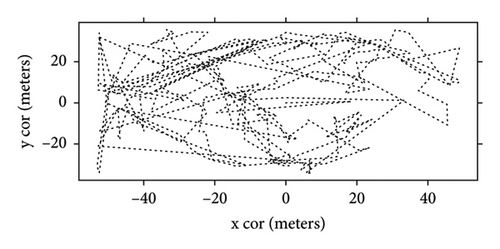
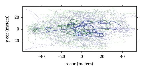
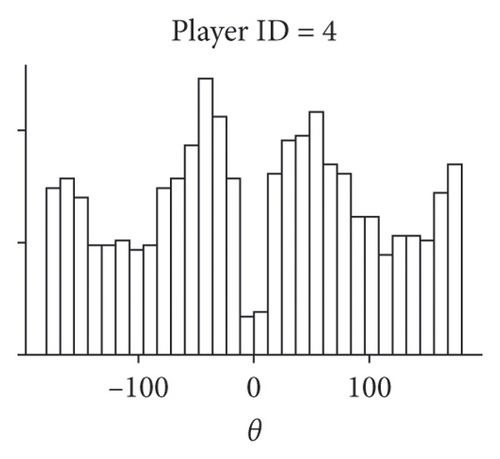
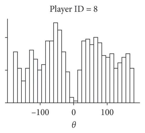
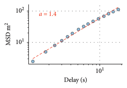
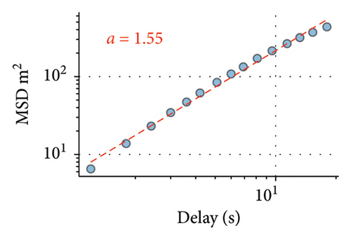
As it is known from statistical mechanics [3, 26], the exponent a relating the square of the displacement and time is informative of the type of motion: while in the case of Brownian motion, the variance of displacement is directly proportional to time, a = 1 values higher than 1 or lower than 1 indicate superdiffusive or subdiffusive motion respectively. Lévy walks are superdiffusive; therefore, their exponents lie in the range 1 < a < 2, between the Brownian motion and the ballistic limit. As the third column of Figure 2 shows, values of a computed for individual players show that their motion is superdiffusive.

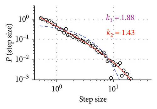
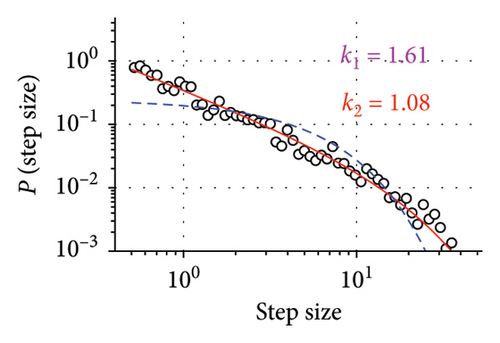
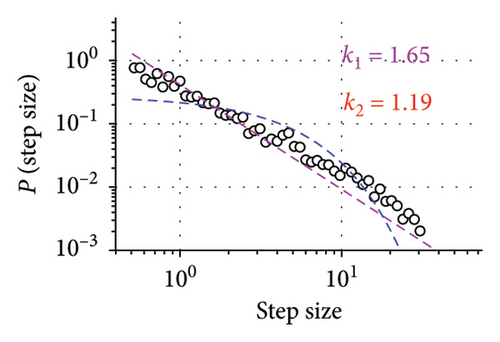
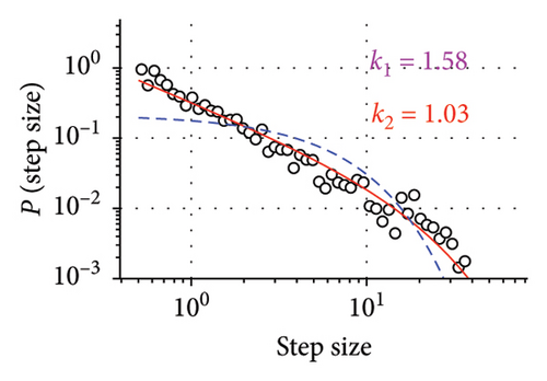
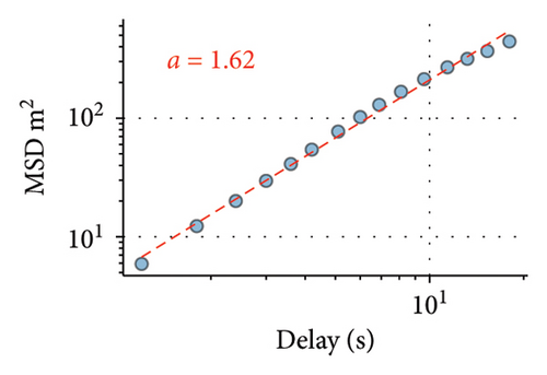
Superdiffusive behavior is a crucial characteristic of the Lévy walk; however, it can be exhibited by other modes of motion. For the definitive test, it is necessary to examine the step size distribution. As the players’ trajectories are continuous and two-dimensional, we implement the methodology developed in [6] for such scenarios. This approach uses the symmetry of Lévy walks: when projected to a lower dimension, Lévy walk retains its properties and remains distinguishable from other modes of movement, such as Brownian motion. Considering the 1D component of trajectory significant turns can be unequivocally determined as reversions of motion in one dimension. Motion in X and Y dimensions are considered separately, as we assume that the rectangular field would impose different constraints on player mobility in vertical and horizontal directions and therefore different values of Lévy walk exponents. Summary statistics for all players, including their Lévy exponents in both X and Y dimensions, are available in the Supporting Information (Tables S1 and S2). Different Lévy exponents for different axes of motion have been previously reported for airborne dispersal of seeds [10], concerning horizontal and vertical dimensions.

The first column of Figure 2 presents the distribution of step sizes for the Y dimension for the goalkeeper (Figure 2(a)) and 3 field players with different roles (remaining panes). We used the maximum-likelihood estimator (MLE) to fit the power law and truncated power law to the data [27] as well as to conduct log-likelihood tests to compare truncated power law with other candidate long-tailed distributions, such as log-normal and exponential (Figure 2). For all players, these tests have shown unambiguously (p > 0.05) that the truncated power law is the best fit for the data. Power law without truncation gives a better fit than the exponential distribution but is superseded by both the log-normal distribution and the truncated power law. Power law scaling extends more than two orders of magnitude in the Y-axis and is close to two orders of magnitude on the X-axis, thus being close to fulfilling the proposed [28] “rule of thumb” for elucidating scale-free phenomena in biological systems. The curtailed scale on the X-axis is caused by the size of the football pith. Values of k₁ and k₂ correspond to the Lévy walk exponent of regular and truncated power laws; they are different for different players; most pronounced is the distinction between the goalkeeper and the field players. As is expected, power law exponents k₁ and k₂ are inversely related to the MSD exponent a.

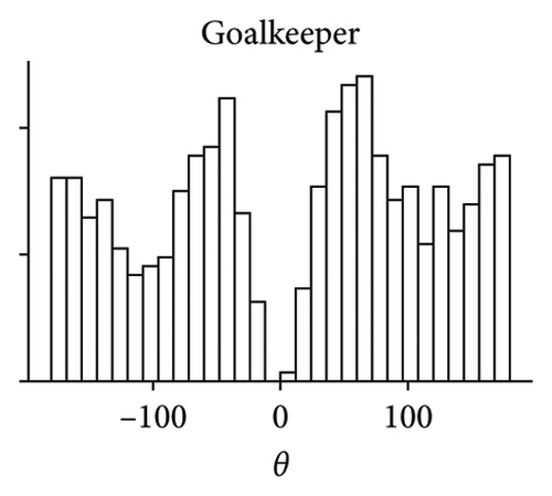
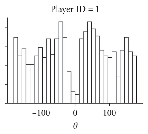
Another characteristic of the true Lévy walk is that the distribution of turning angles between consecutive steps is close to uniform. We use the points previously identified as reversals of 1D motion in the Y dimension to compute the angle direction of movement before and compute players’ turning angles at these points. The turning angle distribution is presented in the central column of Figure 2. Observed distributions could be interpreted as follows: small turning angles are rarely encountered, as the nature of the projection operation eliminated them from data; for θ > 0, the distribution is close to uniform. Uniform turning angle distribution distinguishes Lévy walk from the correlated random walk, which also has superdiffusive properties. Such turning angle distribution has been previously reported for marsupials [11] and wandering albatrosses [6]. Both these species have been found to exhibit Lévy walk behavior with their step size distribution best approximated by truncated power law.

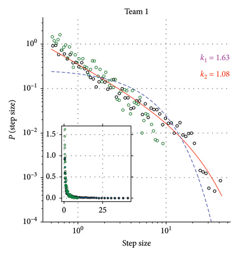
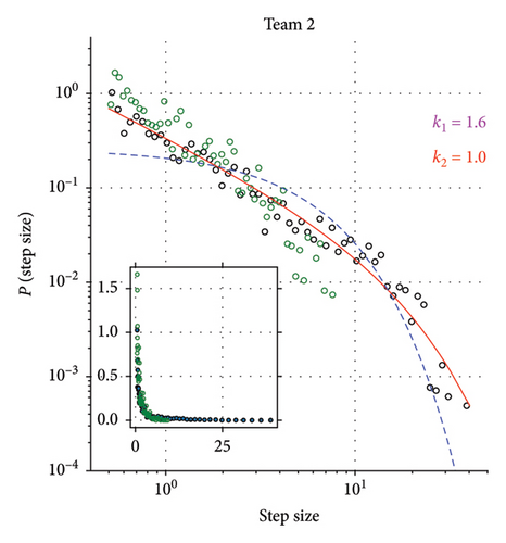
Additionally, we study the distribution of the step sizes for movements of the centers of masses of both teams. We compute the center of mass positions as described previously and then compute the step size distributions for its movements in Y-dimension. We construct surrogate data as a control by performing a circular random shift of individual players’ position time series before computing the team’s center of mass position. These results are presented in Figure 3. An inspection of data presented on logarithmic and linear axes (inset) yields that longer steps are completely absent from the surrogate data. Max-likelihood fits prove that the step size distribution of the real data is best fitted with the truncated power law distribution (p ≪ 0.05) while for synthetic data, exponential distribution presents itself as the more likely candidate, although no clear distinction can be made using log-likelihood tests (p > 0.05). Supporting Information contains an additional simulation study investigating the center of mass trajectory of multiple uncorrelated Levy walks (Figure S3).

2.2. Analysis of Multiple Games

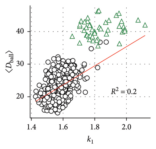
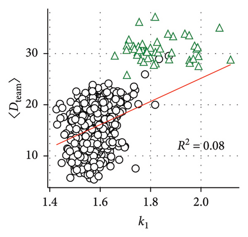
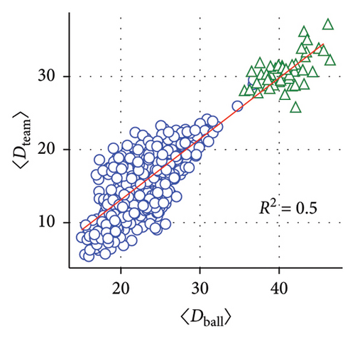
Additionally, we analyze all games contained in the 2022 dataset to elucidate if the Lévy walk exponent is in some way related to the player’s performance or his role in the team. Summarily, 643 individual trajectories of field players and 46 goalkeeper trajectories were analyzed, counting substitute players separately. To acquire insight into the game’s dynamics, for each player, we compute two parameters: the mean distance of the player from the ball 〈D_ball〉 and his mean distance from the center of mass of the team 〈D_team〉. The former is meant to characterize players’ efficiency while the latter serves to quantify their level of involvement in team dynamics. Due to the distinct rules governing the goalkeepers’ movements, we choose to omit their data from the linear regression model, and they are presented on the plots for the visual reference only.

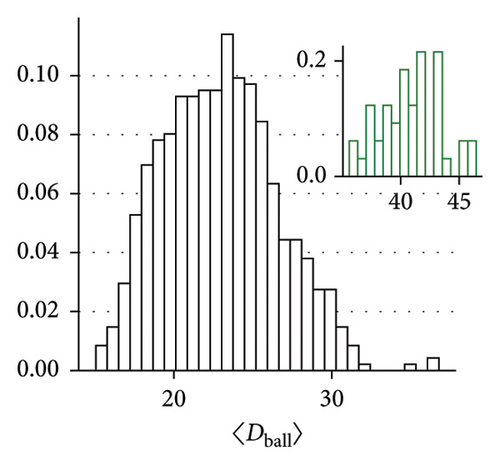
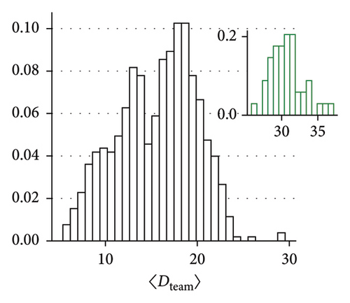
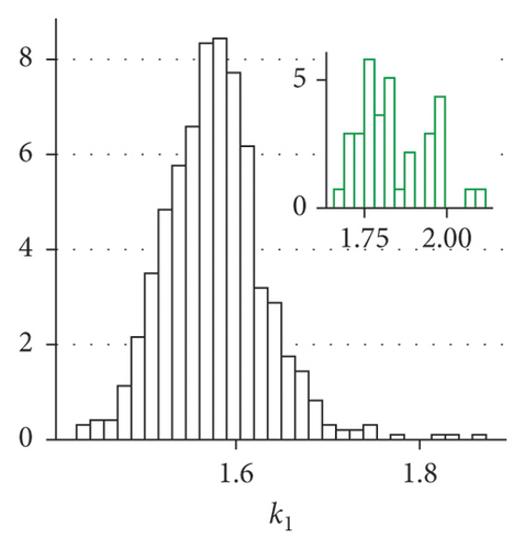
Figures 4(a) and 4(b) demonstrate that a statistically significant relationship exists between the power law exponent of the Lévy walk distribution and the player’s distance to the ball, as well as with his distance to the center of his team (p < 0.05) in both cases. Figure 4(c) shows the relationship between 〈D_ball〉 and 〈D_team〉. As the ball drives the dynamics of the football game, this connection is to be expected. We have found that although the truncated power law provides a better fit to the data, its exponent k₂ has a lesser connection to the player’s dynamics; therefore, k₁, which corresponds to power law fit without truncation, was used. Figures 4(d), 4(e), and 4(f) show the distribution of 〈D_ball〉, 〈D_team〉, and k₁ for all players. All said quantities are distributed normally, as the Kolmogorov–Smirnoff test for normality confirms.

As gaining possession of the ball is a quintessential part of the football game, we investigated if players behave differently when they have the ball, as compared to their movement otherwise during the game. As the properties of the step size distribution do not depend on the specific ordering of elements, it is possible to filter out the steps in which the player had an interaction with the ball and analyze them separately. We used trajectories of all field players to be found in the 2022 dataset and partitioned steps into two categories: steps in which the player had interaction with the ball and all remaining steps. These two aggregate distributions are presented in Figure 5. Some additional information regarding the connection between players’ movement and Lévy exponent is contained in the Supporting Information (Figures S1 and S2).

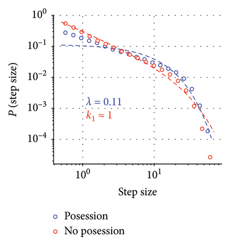
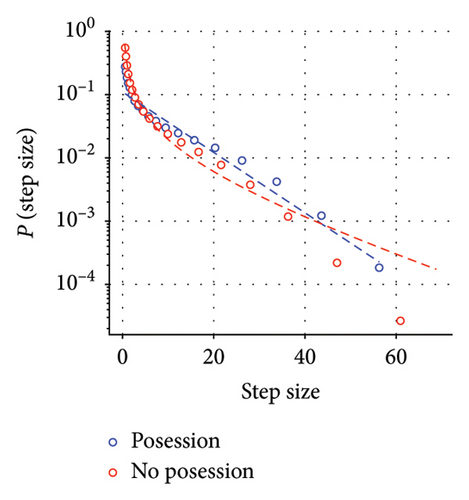
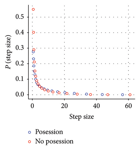
Max-likelihood methods have been used to fit several candidate distributions to the data. It should be noted that although the number of steps is vastly different between these two distributions in both cases, overall, the large number of data points allowed us to obtain confident max-likelihood estimates (p ≫ 0.05) of the best fit. When players are in possession of the ball, the optimal candidate is the exponential distribution; however, when players do not have the ball, truncated power law is the best fit. It should be noted that this distinction is subtle and can only be inferred through log-likelihood tests of the aggregate distribution.

As discussed later, Lévy walk exponent can be seen as an adaptive property for the organisms; therefore, its slope could be influenced by both the player’s skill and their role in the team. In case of, the goalkeepers’, whose movements are constrained by the rules the latter is the case. At the same time, previous research [29] indicates that in human subjects, the exponent changes as the subject becomes more proficient in the task. At this stage, we make no claims whether the observed relationship between the players’ metric and k₁ is determined solely by their role in the team or if it is affected by their skill level as well.

3. Discussion

Lévy walk-like behavior has been repetitively identified in human and animal locomotion. Although some of these findings have been challenged, due to improper data analysis, most of them withstood the most rigorous statistical tests. To the best of our knowledge, Lévy walk has not yet been found in any of the sport’s practitioners, despite the fact that the quantitative analysis of trajectories of professional players is becoming a common practice [19]. Currently, the discourse surrounding the Lévy walk research is shifting from a mere debate regarding its plausibility in human and animal locomotion to a more nuanced discussion of its origin and purpose [2]. Several compelling hypotheses exist to explain the underlying causes of the Lévy walk dynamics. In this work, we explore the conjecture that football games can be seen as a variation of the foraging behavior, as it has been suggested for human hunter-gatherers [14].

The game of football could be viewed as the type of foraging behavior in which agents seek to locate and engage the “resource”—the ball. This conjecture is supported by the observed relationship between 〈D_ball〉 and the power law exponent k₁. At the same time, football is a team endeavor in which individuals seek to coordinate their activity with their teammates and opponents. Some elements of the apparent coordination can be glimpsed from Figure 1, where we see periods of contraction and relaxation as well as evident interdependence between the trajectories of centroids of opposing teams. Intermittent dynamics of contraction and relaxation have been discovered in grazing sheep herd [30] where they serve to balance conflicting imperatives: optimal area coverage provided by the dispersed state and safety in numbers enabled by dense clustering. These oscillations could serve a similar role in teams’ dynamics during the game.

Deviation from the Lévy walk dynamics is observed when we separately consider the step size distributions of players when they are in possession of the ball and otherwise (Figure 5). When players interact with the ball, their aggregate step size distribution is best described by the exponential, as is the case for Brownian motion, and in the second case, the truncated power law distribution is recovered. It is tempting to interpret this result through the prism of the “foraging” approach to the game outlined above: agents resort to the Lévy behavior when they seek to locate and engage the resource; however, when the said resource is acquired, impetus to forage disappears and movement patterns start to resemble Brownian motions. We would, however, be amiss not to mention that there might be a simpler mechanistic explanation to the observed phenomena if the need to interact with the ball constrains the player’s movements thereby making them resemble Brownian walkers. We should note that although similarities can be found between the behavior of football players and that of foraging animals, one should be careful with that analogy as several added levels of behavioral complexity are present in a football game.

Inherent collective effects manifest themselves when we study the motion of the team’s centroids, which also exhibit Lévy walk dynamics. Movement of uncoupled Lévy walkers in a bounded arena results in a Brownian motion of their center of mass (Supporting Information Figure S3). In the context of football game, one expects players’ trajectories to be highly correlated, as the game is inherently a team endeavor [22] and said correlation facilities transference of individual movement patterns on the team level. However, this finding is novel for Lévy walk research, as all previous discoveries concerned the motion of individuals. We interpret our finding as suggestive of the foraging activity performed not by a single individual but by a group, acting to maximize its collective performance. The “resource” could obviously be the ball, which is the foci of players’ efforts; however, it could also be not a material object but a spatial configuration optimal to the needs of the moment. In our view, it would be instructive to investigate if similar phenomena could be observed in animals who practice collective hunting, such as wolves and hyenas.

One way to consider the broader significance of the uncovered phenomena is by invoking the work of Levin [31, 32]. One of his conjectures is that the impetus to understating the functioning of complex systems can be gained by expanding the definition of “Self”: leaving the idea of selfhood as something reserved to a single embodied and cognizant entity, such as a human or animal and entertaining the possibility of expanded or reduced selves, examples of which can be collectives or subsystems of an organism. “Selves” in such a paradigm should be treated as integrated entities capable of pursuing goals by modifying their behavior.

Once such a standpoint is taken concerning the football team dynamics, discovery of Lévy walk—a type of behavior that was previously only found in individuals on the collective level—becomes something that could be anticipated. A football team is an entity that has a goal and can pursue it by modifying its behavior, both during the game and before it in the training process. It comes as no surprise then that the movement strategy that the “Team self” adapts to optimize its performance shares statistical properties with the movement strategies adopted by individual “Selves” who experience similar environmental pressures.

4. Conclusion

In our work, we showed that football players’ trajectories during the game manifest Lévy walk dynamics. Furthermore, Lévy walk exponents, which characterize the preponderance of longer steps in the distribution, are related to the players’ role during the game, and players with lower exponents are on average closer to the ball and explore a larger portion of the field. Curiously, a departure from the Lévy walk behavior is observed, when players are in possession of the ball. Furthermore, power law distribution of step sizes is present in the collective description of players’ activity (center of mass trajectory), an observation novel to the Lévy flight discourse, as it has been centered on the individual trajectory properties. At this stage, we make no definitive claims regarding the generative mechanism of observed behavior; however, we theorize that the scale-free distribution of step sizes is influenced by both the collective nature of the game and its inherent “foraging” premise. Further work should include modeling to elucidate generative mechanisms as well as additional inquiry into the relationship between the Lévy walk exponent and other trajectory metrics and players’ performance. An alternative road for other disciplines might be to study if the elements of foraging present in the football game might explain its widespread popularity.

5. Materials and Methods

We obtained match recordings of Japan’s top football league, J-League, by licensing two datasets from the league’s official data company, DataStadium, Inc. Each dataset contains time-stamped trajectories of players from both teams for the sequence of games in which the season’s winning team participated. The data were acquired using the TRACAB’s optical video tracking systems Gen IV [33]. In brief, this technology relies on gathering optical data from two multicamera units, located at both sides of the midfield line, which is then used to reconstruct players’ trajectories. Ball position is acquired in a separate process: when a player has the ball, his position is taken as a proxy for the ball’s coordinates; in between these events, the position of the ball is obtained by linear interpolation.

The original data format is 25 Hz and the spatial resolution of the recording is in cm. Coordinates of all players from both teams were recorded, as well as the ball trajectory. To investigate if the temporal resolution of the data affects the results, we have created several downsampled datasets with temporal resolution ranging from 1 Hz to 25 Hz and repeated our analysis. No statistically significant differences were observed between different downsamplings of the data.

All computations for the paper have been performed using custom scripts written in Python programming language and are available from authors upon reasonable request. For fitting the power law distribution to the data and performing log-likelihood, powerlaw Python package was used [27]. x_min value was set to 0.5 m, to exclude potential spurious fluctuations. Steps with lengths below the threshold were excluded from the analysis. To investigate how the threshold value x_min affects the result, we repeated our analysis using a range of threshold values: 0.5 < x_min < 5 m. As it is expected, the choice of threshold affects the value of the exponents k₁ and k₂, and once a sufficiently high threshold value is used, the power law distribution is reduced to the exponential. We have found that for most players, when x_min < 4 m, the power law scaling is retained.

To filter out the steps in which the player had interacted with the ball, after partitioning the trajectory into steps using the 1D projection, we computed the minimal distances between the player and the ball for each step separately. If said distance was 0.15 m at least once, it was considered that a player had possession of the ball during that step. On average, field players interact with the ball for 9% of their steps [34].

Disclosure

This manuscript was submitted as a preprint in the link https://www.biorxiv.org/content/10.1101/2024.06.11.598528v2.

Conflicts of Interest

The authors declare no conflicts of interest.

Funding

This work was supported by Japan Science and Technology Agency (Grant Number JPMJPF2205).

Supporting Information

Attached to this paper are the supplementary materials that contain Tables S1 and S2 with the Lévy exponents in the X and Y dimensions for all players analyzed in the section “Analysis of a Single Match” and Table S3 with summary information on all games contained in the dataset. Additional figures present the relationship between the area of convex hull for each player (Figure S1) and dependence of the Lévy exponent on players’ position in the field (Figure S2). The figures are accompanied with short discussion of their meaning and relevance. Results for additional simulation study concerning the behavior of Lévy walkers on the bounded arena are presented in Figure S3.