A Detailed Study of ABC-Type Fractal–Fractional Dynamical Model of HIV/AIDS
Abstract
This paper is aimed at studying the dynamics of community transmission of HIV by constructing a fractal fractional mathematical model whose kernel is a generalized Mittag–Leffler type. First, we collect and analyze statistical data for epidemiological surveillance of HIV/AIDS prevalence in Yemen from 2000 to 2022. Then, we employ the statistical analysis software EViews and apply ARIMA models to predict the number of HIV/AIDS cases from 2023 to 2024. The results of the selected model, free of standard problems, predicted a future increase in HIV/AIDS cases in Yemen. Next, relying on the well-known fixed-point theorem and a set of other associated results, we prove the existence and uniqueness results of the fractional model. Moreover, we use the Adams–Bashforth method to approximate the solutions of this system numerically. Finally, we plot, tabulate, and simulate our results using the Mathematica software and compare them to the results obtained from the statistical model.
1. Introduction
The first global incidence of HIV infection was reported on June 6, 1981 [1]. As we presently know today, the transmission of HIV occurs through semen, blood, breast milk, and vaginal secretions (cervical). HIV breaks down an infected individual’s immune system and finally converts it into acquired immune deficiency syndrome (AIDS) because the afflicted person is ignorant of the protection system and lacks active medical treatment [2, 3]. HIV and AIDS are closely related but distinct conditions that have profoundly impacted global health since their discovery. HIV has infested millions of individuals since the outbreak of the AIDS pandemic, and the number is growing by the day [4]. Depending on an individual’s physical condition, the transition from HIV to AIDS can occur over many years. Specific behavioral factors may increase the likelihood of infection when contacting an HIV-positive person [5]. Risk factors involve sharing unclean needles or syringes, having unprotected sex, and using nonsterile equipment for medical proceedings, blood transfusions, and tissue transplants. In addition to these contributing factors, certain groups of individuals, like sexual workers, men who have sex with men (MSM), transgender, bisexuals, gay, male sexual workers (MSWs), female sex workers (FSWs), and persons who inject drugs (PWIDs), are constantly at a high probability of contracting HIV [6]. Prevention activities focus on educating people about how HIV spreads and promoting safe behaviors, including using condoms, getting tested, and knowing one’s HIV status. Furthermore, extremely effective medications known as antiretroviral therapy (ART) can slow the progression of HIV, boost the immune system, and reduce the risk of transmission to others [7]. HIV/AIDS remains a significant threat to public health. Therefore, healthcare providers and researchers must comprehend and anticipate the incidence of HIV/AIDS.
On the other hand, Kurniasari et al. conducted the autoregressive moving average (ARMA) model to predict HIV infection cases in Indonesia from 2019 to 2030. The results showed that the optimal model is ARMA (1,1) and that infection cases are expected to increase from 22,679 in 2019 to 36,255 in 2030 [8]. Luo et al. aimed to use the seasonal autoregressive integrated moving average (SARIMA) model to predict the incidence of AIDS in Henan Province, China. Monthly infection rate data from January 2012 to December 2019 and from January 2020 to December 2020 were used for verification. The findings revealed that the monthly prevalence of AIDS varied from 0.05 to 0.50 per 100,000 people, with a specific periodicity throughout Henan Province [9]. Yu et al. presented the autoregressive integrated moving average (ARIMA) model to predict HIV infections from 2013 to 2017 based on infection data from 1985 to 2012. The results showed that the optimal prediction model is ARIMA (1,2,2), where HIV infections were 1111 in 2017, with a confidence interval of 95% [10]. Wang et al. developed an effective HIV/AIDS prevalence prediction model in Guangxi Province, China. HIV incidence data from 2005 to 2016 and 2015 and 2016 were used to check which models were most appropriate. The study used the ARIMA model, long short-term memory (LSTM) neural network models, exponential smoothing (ES), and general regression neural network (GRNN). The LSTM model outperformed other time series techniques and is critical for local HIV surveillance and control of epidemics [11]. Purwanto et al. proposed a good adaptive neuro-fuzzy inference system (ANFIS) model for predicting HIV/AIDS infection data. The study used two statistical indexes, root mean square error (RMSE) and mean absolute error (MAE), to compare the proposed model’s prediction results with those obtained with ARIMA models. According to the findings, the revised ANFIS model best suits HIV/AIDS time series forecasting [12]. Nisa et al. presented a prediction model utilizing patients’ electronic medical information in Nai Zindagi Trust (NZ), Pakistan. The prediction model for the likelihood of future HIV infection has been validated in high-risk groups. They analyzed demographic, social, and behavioral data (sexual behavior and drug injection) and biological factors to predict which patients are at high risk of contracting HIV [4]. Li et al. presented a susceptible–exposed in the latent stage–infectious (SEI) model as a means to comprehend the progression of the HIV/AIDS pandemic in China. The determination of the basic reproduction number was conducted within the framework of the SEI model, which serves as a valuable tool for understanding the dynamics of disease transmission [13]. A mathematical model was built by Ayele et al. to address the issue of HIV/AIDS in Ethiopia. The study investigates optimum control measures for prevention, screening, and treatment of the disease [14]. Levy et al. created a time-dependent stigma function using a data-driven methodology to measure the population’s internalized and performed stigma. They included this in their compartmental HIV dynamics model, and they rescaled their model system to create a coupled system for HIV prevalence and the fraction of individuals who are infected and seek treatment. That allowed them to estimate model parameters from published data [15]. In [16], the authors provided a nonlinear mathematical model of HIV/AIDS transmission dynamics in Cuba.
Statistical modeling, a powerful tool in epidemiology and public health, is critical when investigating the dynamics of HIV/AIDS transmission and potential future trends. The ARIMA program is crucial for predicting the occurrence of HIV/AIDS because it uses previous data to generate insights and forecast future trends [9, 17]. This predictive capability is vital for public health planning. It helps authorities anticipate when new cases will likely occur, allowing for timely interventions and healthcare provision.
In recent times, fractional calculus and its diverse applications have witnessed remarkable advancements. Numerous numerical and analytical methods have been formulated to tackle the challenges posed by fractional calculus (see [18–22]).
Fractional differential equations (FDEs) are used as a mathematical framework to explore physical and biological processes that exhibit memory effects or extended dependencies within their system [23–25]. Including fractional-order derivatives in these equations allows an accurate representation of the complex dynamics in systems that display nonlocal or non-Markovian characteristics. In this context, it is clear that FDEs play a crucial role as useful tools in studying the stability of mathematical models and analyzing and understanding the complex dynamics that govern a wide range of biological processes. For further details, refer to [26, 27]. A substantial body of academic work has thoroughly explored the application of FDEs in modeling and interpreting the dynamics of biological systems, as highlighted in the research by Lu [28]. Similarly, Aldwoah et al. [29] investigated a mathematical and statistical model of malaria transmission dynamics in Yemen, utilizing piecewise Caputo–Fabrizio derivatives. In 2017, Atangana [30] introduced a new class of operators called fractional operators that combined concepts from fractional and fractal calculus. These operators integrate power laws, exponential laws, and generalized Mittag–Leffler functions with fractal derivatives. The operators have two key components: a fractal order and a fractal dimension. FDEs can translate the order and dimension of a system into a rational framework. The primary motivation is to enable analysis of nonlocal boundary or initial value problems exhibiting fractal properties. Early results show the generalized fractal operators provide more accurate simulations of real-world phenomena with fractal and nonlocal characteristics than traditional methods. Some recent works have further developed the foundations and applications of Atangana’s fractal operators in models requiring fractional and fractal calculus concepts [31–33]. Overall, the fractal operators pioneered by Atangana significantly extend fractional calculus’ capabilities for fractal system modeling across scientific domains. The Atangana–Baleanu fractional derivative operator offers an enhanced modeling framework compared to prior fractional derivatives. It possesses beneficial mathematical properties like allowing analytical solutions and numerical approximations. Additionally, the fractional order and new parameters in the operator have a clear physical meaning related to system heterogeneity and nonlocal characteristics. This robust mathematical foundation and interpretable physical parameters make the Atangana–Baleanu derivative well-suited for accurately modeling complex fractional-order processes arising in real-world systems.
Given the innovative nature and demonstrated capabilities of fractal operators, we develop a mathematical model of HIV/AIDS infection using Atangana–Baleanu fractal derivatives. The development and analysis of such a nonlocal fractal model of HIV infection will provide new insights into disease progression and prediction; this represents an original contribution demonstrating fractional calculus’s modeling capabilities in an important biomedical application.
This paper’s novelty lies in its innovative approach to modeling using fractal–fractional order derivatives, detailed analysis of the memory effect, and reliance on the combination of statistical and mathematical methods to analyze and conclude the data under study.
This paper is organized as follows: Section 2 reviews relevant literature. The statistical model is described and analyzed in Section 3. In Section 4, some definitions and formulations of the mathematical model are presented. The existence and uniqueness of the solution for the proposed model are proven in Section 5. The model’s approximate solution is found in Section 6. The numerical solution and model simulations through parameter estimation are discussed in Section 7. In the final section, we present conclusions and recommendations.
2. Statistical Results
This section is dedicated to examining the gathered statistical data concerning the total instances of HIV/AIDS in Yemen [34]. Furthermore, it is aimed at forecasting future occurrences of HIV/AIDS transmission to alert decision-makers and experts to the necessity of monitoring and combating this issue. A brief discussion of the key findings is also provided.
2.1. Descriptive Data Analysis
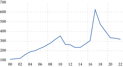
Table 1 presents the confirmed instances of HIV/AIDS, as derived from epidemiological surveillance data released by the Central Bureau of Statistics. We found fluctuations in the total number of infected cases. There was a consistent rise in the total infection cases, escalating from 110 cases in 2000 to 354 cases in 2010, signifying an increase of 221.8%. After that, there was a decline in the incidence of HIV/AIDS from 266 cases in 2011 to 232 cases in 2014, representing a relative decrease of 12.8% from 2011 to 2014. Conversely, there was a resurgence between 2015 and 2017, culminating in 628 cases in 2017. Following this, there was a consistent decline from 2018 to 2022. In general, we found that the total number of HIV/AIDS infections escalated from 110 cases in 2000 to 317 cases in 2022, marking an increase of 188% over the period under study from 2000 to 2022. This trend is graphically represented in Figure 1.
| Years | HIV/AIDS cases |
|---|---|
| 2000 | 110 |
| 2001 | 117 |
| 2002 | 122 |
| 2003 | 158 |
| 2004 | 188 |
| 2005 | 202 |
| 2006 | 223 |
| 2007 | 248 |
| 2008 | 277 |
| 2009 | 318 |
| 2010 | 354 |
| 2011 | 266 |
| 2012 | 261 |
| 2013 | 232 |
| 2014 | 232 |
| 2015 | 271 |
| 2016 | 303 |
| 2017 | 628 |
| 2018 | 473 |
| 2019 | 403 |
| 2020 | 336 |
| 2021 | 329 |
| 2022 | 317 |
2.2. Forecasting Strategy
The primary objective and advantage of employing time series models are to utilize them in estimating the variables’ conduct and diverse phenomena and their prospective trends in fields such as epidemiology, disease study, economics, climate sciences, management, and other scientific disciplines [35, 36]. Recently, the behavior and patterns of several diseases and epidemics have been predicted using statistical and mathematical modeling. These models encompass four fundamental procedures for the forecasting process: identifying the model, subsequently estimating the unknown parameters, and following the diagnostic process, and the final phase entails the process of prediction [37, 38]. Models such as moving average (MA), autoregressive (AR), generalized autoregressive conditional heteroskedasticity (GARCH), autoregressive conditional heteroskedasticity (ARCH), ARIMA, and ARMA are among the most frequently utilized time series models for forecasting purposes [39, 40]. The collected data on HIV/AIDS cases from 2000 to 2022 was thoroughly analyzed. The stability of this data was scrutinized through assumptions and tests to ensure its validity for future predictive modeling. Calculating coefficients (partial autocorrelation function (APCF) and autocorrelation function (ACF)) and implementing unit root tests such as augmented Dickey–Fuller and Phillips–Perron have indicated that the time series under consideration is unstable; this suggests the presence of a discernible general trend, as depicted in Figure 1.
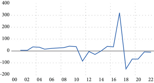
As illustrated in Figure 2, we used the time series data’s first differences for the forecasting procedure. Regarding the unit root test, the computed values surpass the critical values across all confidence levels, as depicted in Table 2. The probability values (Prob. = 0.00) fall below the 5% significance level. Consequently, the null hypothesis, which posits that the time series possesses a unit root, can be rejected. The alternative hypothesis, suggesting that the time series does not have a unit root, is thus accepted. Therefore, the time series representing HIV/AIDS cases demonstrates stationary after applying the first differences.
| Test critical values | |||||
|---|---|---|---|---|---|
| Test | T -statistic | Prob. | 0.01 | 0.05 | 0.10 |
| Phillips–Perron | −4.990581 | 0.0035 | −4.467895 | −3.644963 | −3.261452 |
| Augmented Dickey–Fuller | −4.966336 | 0.0036 | −4.467895 | −3.644963 | −3.261452 |
Additionally, we analyzed the autocorrelation and partial autocorrelation functions, and we suggest the models for predictive purposes. The suggested models’ coefficients were estimated using the ordinary least squares (OLS) method. The ARIMA (1,1,0) model was chosen as the most optimal based on specific criteria. These criteria included the statistical significance of the model’s coefficients, a coefficient of determination that surpasses that of other models, the smallest variance, less volatility, and the lowest value of the Akaike information criterion (AIC) indicator, as demonstrated in Table 3.
| ARIMA models | SIGMASQ | Adjusted R2 | AIC | SC |
|---|---|---|---|---|
| ARIMA (1,1,0)a | 6.21 | 0.49 | 11.86 | 12.01 |
| ARIMA (1,1,1) | 6.24 | 0.42 | 11.95 | 12.15 |
| ARIMA (0,1,1) | 8.33 | 0.31 | 12.14 | 12.29 |
| ARIMA (1,1,2) | 6.45 | 0.33 | 12.57 | 12.85 |
| ARIMA (4,1,1) | 7.65 | 0.35 | 12.06 | 12.24 |
| ARIMA (0,1,2) | 6.85 | 0.38 | 12.51 | 12.35 |
- aThe optimal model among all the models shown in the other rows of the table.
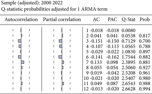
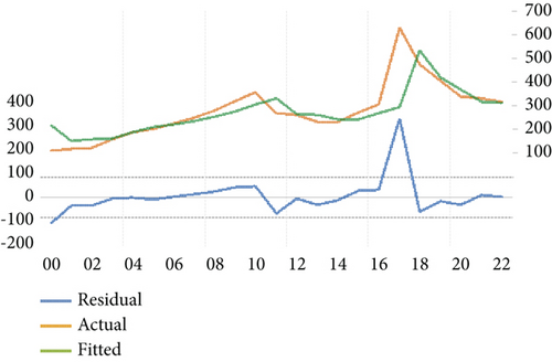
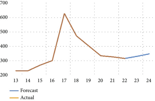
Furthermore, we scrutinized the optimal model via a residual test to ascertain the alignment between the original observations and the estimated values derived from the candidate model and to validate the model’s hypotheses. The robustness of the suitability of the chosen statistical model was also confirmed through the randomness of residuals, the shape of the autocorrelation, and partial autocorrelation functions. Figure 3 indicates an absence of autocorrelation among errors. In other words, autocorrelation and partial autocorrelation fall within confidence limits, suggesting that the residuals can be characterized as white noise. The congruence between the estimated and actual values was verified by graphically representing them, as depicted in Figure 4. This illustration not only demonstrates the proximity of the estimated values to the actual ones but also attests to the quality of the model. The chosen and problem-free ARIMA (1,1,0) model was utilized to forecast the patterns and future trends of the total number of HIV/AIDS-infected persons. The model projected an escalation in infection cases in Yemen, as shown in Figure 5.
3. The Formulation of the HIV/AIDS Model
This section uses some basic definitions and notions for the proposed model.
Definition 3.1 ([30]). Let Ψ(t) be continuous in (a′, b′), if Ψ is fractal differentiable on (a′, b′) with order μ, then the fractal–fractional derivative of Ψ of order τ in the Riemann–Liouville sense with exponential decay kernel is given as
Definition 3.2 ([30]). If Ψ(t) is continuous in an opened interval (a′, b′), then the fractal–fractional integral of Ψ(t) with order τ is defined as
Taking into account not to change the parameters imposed in Model (3),is the fractal fractional derivative of orderτand fractal orderμvia the ML-type kernel, and bothτ ∈ (0, 1) and μ ∈ (0, 1].
4. Existence and Uniqueness of Solution
In this section, we prove the existence of solutions for Model (4) by using fixed-point theory. LetEbe a nonempty set in Banach space,E ∈ H4, whereH ∈ C(J, R) with norm ‖N‖E = ‖S, U, D, A‖E = max|Z(t)|, t ∈ J, for |Z| = |S| + |U| + |D| + |A|.
Theorem 4.1 ([41]). Let E be a Banach space, a convex closed bounded set, V a subset of an open set, and 0 ∈ V. Then, for the continuous and compact map , either
- 1.
∃v ∈ V s.t. v = F(v) or
- 2.
∃v ∈ ∂V and 0 < α < 1 s.t. v = αF(v)
Theorem 4.2. Let K ∈ C(J × E, E); assume that
A1. ∃ℵ ∈ L1(J, R+) and ∃G ∈ C([0, ∞), (0, ∞)) s.t. ∀t ∈ J and Ξ ∈ E, |K(t, Ξ(t))| ≤ ℵG|(Ξ(t))|
A2. ∃β > 0 s.t.
Then, the solution of Model (4) and then for Equation (7) exists on J.
Proof 1. Let F : E⟶E and assume Wr = {Ξ ∈ E : ‖Ξ‖E ≤ r}, r > 0. As K is continuous, so too is F. From A1, we obtain
For Ξ ∈ Wr,
Thus, F is uniformly bounded on E. Now, we set , and Ξ ∈ Gr. For t, u ∈ [0, T] s.t. t < u, we find
As u⟶t, we see that the expression ‖F(Ξ(t)) − F(Ξ(u))‖E⟶0. This gives the equicontinuity of F. Accordingly, the compactness of F on Wr is deduced by the Arzelá–Ascoli theorem. Since all conditions of Theorem 4.1 are fulfilled on F, we have one of (1) or (2). From A2, we set p = {Ξ ∈ E : ‖Ξ‖E < ν}, for some ν > 0 s.t.
From A1 and (Equation (14)), we get
Assume that there are Ξ ∈ ∂P and 0 < δ < 1 s.t. Ξ = δF(Ξ). Then, by the above inequality, we obtain
This contradicts our hypothesis (A2). Hence, F has a fixed point in p by Theorem 4.1. This demonstrates that a solution to Fractal–Fractional Model (4) exists.
Now, we prove the uniqueness result of Model (4).
Lemma 4.1. Let S, U, D, A, S⋆, U⋆, D⋆, A⋆ ∈ C(J, R), and let ‖S‖ ≤ w1, ‖U‖ ≤ w2, ‖D‖ ≤ w3, ‖A‖ ≤ w4, where w1, w2, w3, w4 ∈ R+. Then, the kernels K1, K2, K3, K4 defined in Equation (5) satisfy the Lipschitz condition.
Proof 2. For K1, let S, S⋆ ∈ C(J, R). Then,
Theorem 4.3. Assume that Lemma 4.1 holds. Then, Model (4) has exactly one solution if
Proof 3. Suppose that there is another solution for Model (4), namely, (S∗(t), U∗(t), D∗(t), A∗(t)), with initial conditions (S∗(0) = S0, U∗(0) = U0, D∗(0) = D0, A∗(0) = A0).
By using the Equation (11), we have
It follows that
The above inequality holds if ‖S − S∗‖ = 0 or S = S∗. By the same way, we can prove that U = U∗, D = D∗, and A = A∗. So (S(t), U(t), D(t), A(t)) = (S∗(t), U∗(t), D∗(t), A∗(t)). Thus, Model (4) has a unique solution.
5. Numerical Treatment
6. Discussion and Numerical Results
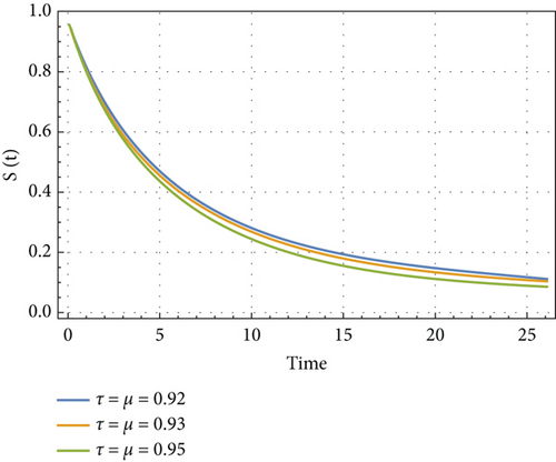
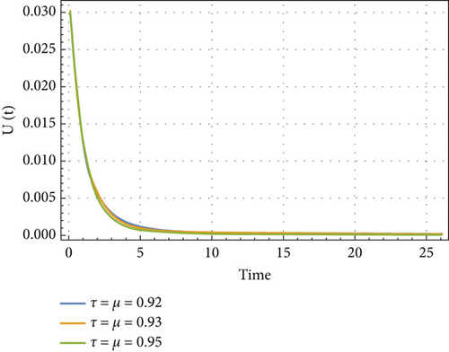
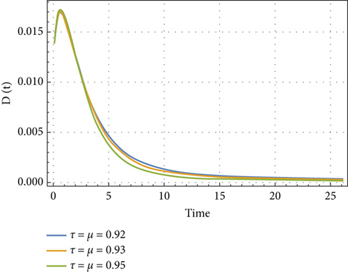
In this part, we use actual data for the parameters and beginning values assumed by [16] to simulate and describe the dynamic behaviors of the Fractal–Fractional HIV/AIDS Model (4). We assume that a = 0.01, b = 0.5, c = 0.2, d = 0.13, e = 0.5, f = 0.8, and h = 0.1 based on the information in this source. In addition, the starting real values obtained from the Health Office of the Republic of Yemen are as follows: S(0) = 0.94, U(0) = 0.03, D(0) = 0.0014, and A(0) = 0.006.
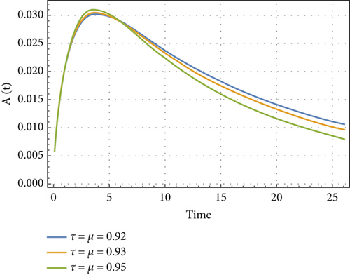
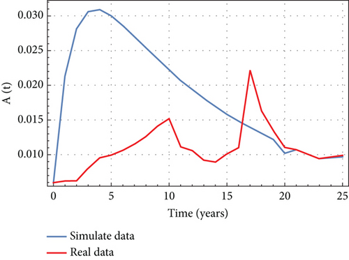
In Figures 6, 7, 8, and 9, we analyze the behavior of the functions S, U, D, and A under the influence of different fractional orders (τ = μ = 0.92,0.93,0.95), using the Adams–Bashforth method. The results presented in Table 4 illustrate the number of individuals diagnosed with HIV/AIDS over the past 24 years. These simulations highlight the significant role of memory effects introduced by fractal- and fractional-order derivatives, which contrast sharply with the behavior observed when ordinary derivatives are used within this model. We analyzed the results obtained from the approximate solution of the given model for different values of μ and τ, as shown in Table 4. At μ = 0.95, the results closely matched the statistical data of reported cases in Yemen from 2000 to 2024. As highlighted in Table 4, it is noteworthy that the mathematical and statistical results align well from 20 to 24 years. Using Table 5, we compared the approximate solution at μ = 0.95 with the results depicted in Figure 5. This comparison is illustrated in Figure 10.
| Orders | |||
|---|---|---|---|
| τ = μ = | 0.91 | 0.93 | 0.95 |
| Time | A(t) | A(t) | A(t) |
| 0 | 0.006 | 0.006 | 0.006 |
| 1 | 0.021 | 0.021 | 0.021 |
| 2 | 0.0241 | 0.0214 | 0.028 |
| 3 | 0.0298 | 0.0301 | 0.0306 |
| 4 | 0.0302 | 0.0304 | 0.0309 |
| 5 | 0.0297 | 0.0298 | 0.0300 |
| 6 | 0.0288 | 0.0287 | 0.0286 |
| 7 | 0.0274 | 0.0273 | 0.0270 |
| 8 | 0.0261 | 0.0259 | 0.0254 |
| 9 | 0.0248 | 0.0245 | 0.0238 |
| 10 | 0.0236 | 0.0231 | 0.0222 |
| 11 | 0.0223 | 0.0218 | 0.0207 |
| 12 | 0.0212 | 0.0206 | 0.0194 |
| 13 | 0.0208 | 0.0194 | 0.0181 |
| 14 | 0.0190 | 0.0183 | 0.0169 |
| 15 | 0.0180 | 0.0173 | 0.0158 |
| 16 | 0.0171 | 0.0164 | 0.0148 |
| 17 | 0.0163 | 0.0155 | 0.0139 |
| 18 | 0.0155 | 0.0146 | 0.0130 |
| 19 | 0.0147 | 0.0139 | 0.0122 |
| 20 | 0.0140 | 0.0131 | 0.0114 |
| 21 | 0.0133 | 0.0124 | 0.0107 |
| 22 | 0.0127 | 0.0118 | 0.0101 |
| 23 | 0.0121 | 0.0112 | 0.0094 |
| 24 | 0.0115 | 0.0106 | 0.0096 |
| Order | |
|---|---|
| τ = μ = 0.95 | |
| Time | A(t) |
| 0 | 0.006 |
| 1 | 0.021 |
| 2 | 0.028 |
| 3 | 0.0306 |
| 4 | 0.0309 |
| 5 | 0.0300 |
| 6 | 0.0286 |
| 7 | 0.0270 |
| 8 | 0.0254 |
| 9 | 0.0238 |
| 10 | 0.0222 |
| 11 | 0.0207 |
| 12 | 0.0194 |
| 13 | 0.0181 |
| 14 | 0.0169 |
| 15 | 0.0158 |
| 16 | 0.0148 |
| 17 | 0.0139 |
| 18 | 0.0130 |
| 19 | 0.0122 |
| 20 | 0.0114 |
| 21 | 0.0107 |
| 22 | 0.0101 |
| 23 | 0.0094 |
| 24 | 0.0096 |
7. Conclusion
We have comprehensively studied the dynamics of HIV transmission in the community by constructing a fractal–fractional mathematical model whose kernel is a generalized Mittag–Leffler type. On the statistical aspect, we have analyzed the statistical data on HIV/AIDS cases in Yemen from 2000 to 2022. A significant surge in HIV/AIDS cases was noted in 2022, with an increase of 188% compared to 2000. Then, the ARIMA model to forecast future trends and patterns of HIV/AIDS has been applied. The model’s predictions have indicated a continued rise in the number of individuals infected with HIV/AIDS, with estimates of 332 and 349 cases for 2023 and 2024, respectively. In the theoretical analysis, we have established the existence and uniqueness of the solutions based on the fixed-point theory and some nonlinear analysis results. Numerically, the Adams–Bashforth method has been used to solve the proposed model. Moreover, the given results have been tabulated, plotted, and simulated using the Mathematica program and compared with the results obtained from the statistical model. The study results confirmed there is a consistency that cases of HIV/AIDS infection will continue to increase in the two models for the years 2023 and 2024. The statistical analysis of HIV/AIDS cases in Yemen from 2000 to 2022 may have limitations. Data availability, quality, and reporting biases could affect the reliability of statistical models and forecasts. Theoretical analysis may have limitations in applicability due to parameter uncertainties and population dynamics. In light of these limitations, further research incorporating more comprehensive data, refining modeling approaches, and considering additional factors influencing HIV transmission dynamics would be valuable for improving the accuracy and reliability of predictions and informing effective public health strategies in Yemen and beyond. This is what we are going to do in the upcoming research.
Conflicts of Interest
The authors declare no conflicts of interest.
Funding
There is no funding provided for this work.
Acknowledgments
This work was conducted during our work at Hodeidah University.
Open Research
Data Availability Statement
The data used have been included in the paper.


