A Novel Machine and Deep Learning–Based Ensemble Techniques for Automatic Lung Cancer Detection
Abstract
Lung cancer (LC) remains one of the most challenging malignancies to diagnose accurately due to the complexity of its pathology and the limitations of traditional diagnostic protocols. This study presents a novel deep learning–based ensemble technique aimed at enhancing the automatic detection of LC, integrating machine learning (ML) methodologies to improve diagnostic accuracy and reliability significantly. The publicly available Kaggle LC survey dataset, comprising 309 instances with 16 clinical attributes, including age, smoking history, and symptoms were used. The synthetic minority oversampling technique (SMOTE) for data balancing, complemented by fivefold cross-validation strategy to assess the performance of various ML models, was also employed. This approach utilizes convolutional neural networks (CNNs) integrated with ensemble learning to develop two novel models, ConvXGB and ConvCatBoost, which synergistically combine CNN-based feature extraction with the powerful classification capabilities of XGBoost and CatBoost, respectively, for binary classification in LC detection. ConvXGB achieved improved results, including an accuracy of 98.26%, precision of 98.72%, recall of 98.72%, and F1-score of 98.72%. Such performance metrics underscore ConvXGB’s potential to minimize false positives and negatives, enhancing outcomes in LC diagnostics. Additionally, the complexities surrounding LC diagnosis through a comprehensive comparative analysis were explored, establishing benchmarks for evaluating diagnostic precision, accuracy, recall, and F1-score. Our findings highlight the transformative impact of ML in LC research, paving the way for diagnostic frameworks that promise significant advancements in oncological practices.
1. Introduction
Lung cancer (LC) is a pervasive global malignancy that remains a leading cause of cancer-induced fatalities, posing significant challenges due to its heightened intratumor heterogeneity and the intricate characteristics of cancer cells [1]. With an annual diagnosis rate of 2.20 million individuals, a staggering 75% succumb within 5 years [2]. Overcoming these challenges requires a comprehensive understanding of LC patterns, diagnoses, and treatment responses. When breath is taken, air follows a journey through the body before it reaches the lungs. It first enters through the nose, then travels down the pharynx, through the larynx, and into the trachea [3]. From there, it moves into the bronchi, which split into smaller branches, eventually reaching tiny air sacs called alveoli. These alveoli are surrounded by tiny blood vessels called capillaries, where the magic happens: oxygen from the air breathed enters the blood, and carbon dioxide from our blood is transferred to the alveoli to be exhaled [4]. This exchange is crucial for our survival, as our body relies on a constant supply of oxygen, which it gets through breathing [5]. Understanding this process is essential when studying lung function, especially in the context of early LC detection [6].
Lung diseases sit at the top of the causes of death across numerous developed nations. Lung tissue suffers severe damage as time passes because of exposure to environmental toxins together with smoking and persistent inflammation [7, 8]. The lungs have natural defenses, with mucus as a barrier to trap and remove harmful substances. However, these protective mechanisms can become overwhelmed, especially when someone smokes [9]. The constant exposure to smoke and toxins can damage the lungs’ ability to clear out these harmful particles, making it harder for the body to protect itself. This is one of the reasons why smoking can lead to serious lung conditions over time [10]. Multiple factors including environmental elements together with genetic characteristics and hereditary medical conditions lead to lung health decline which results in different respiratory ailments [11]. Patients who experience chronic obstructive pulmonary disease (COPD) have either chronic bronchitis or emphysema since these two conditions create the overall illness known as COPD [12]. COPD develops when chronic bronchitis joins with emphysema and creates this advanced and progressively worsening illness. Smoking stands as the primary cause leading to the development of this illness [13].
Chronic bronchitis causes persistent inflammation together with bronchi lining damage in the structure that links the trachea to the lungs [14]. Objects with chronic bronchitis present both a prolonged cough along with an abundance of mucus while also causing breathing problems. The main damage target for emphysema occurs within the air sacs of the lungs. The condition produces symptoms that involve continuous coughing, breathing difficulties, reduced physical tolerance, and diminished capacity to execute regular tasks without experiencing fatigue [15].
LC proves to be the leading cancer-related killer for men and women in the United States [16]. The number of deaths from LC exceeds the total deaths from colon cancer, along with cervical cancer and breast cancer combined [17]. A persistent cough stands as the main sign that people with LC experience, and healthcare providers must evaluate this symptom closely. People who currently have COPD from smoking already experience recurrent coughing because of their smoking history [18]. The most critical warning signal related to LC includes a noteworthy change in cough behavior that becomes both more common and more intense and could include mucus production or the presence of blood. The symptoms of LC can manifest as phlegm in coughed-up material alongside chest pain and difficult breathing, as well as appetite reduction and unintended weight loss, as well as fever, along with rare events of hemoptysis [19].
LC stands as a leading cause of cancer-related fatalities worldwide, accounting for 11.4% of new diagnoses and contributing to 18% of all cancer deaths, with approximately 85% attributed to non–small cell lung cancer (NSCLC) [20]. The diagnosis of NSCLC typically entails methodologies such as radiofrequency and stereotactic body radiotherapy (SBRT), unlike small cell lung carcinoma (SCLC), which necessitates specific therapeutic strategies and displays quicker dissemination [21]. NSCLC advances slowly and presents diverse subtypes like squamous cell carcinoma, large cell carcinoma, and adenocarcinoma [22]. Despite radon exposure, smoking, and air pollution being prevalent triggers, NSCLC can impact nonsmoking individuals as well. Indications may encompass a persistent cough, breathing difficulties, chest discomfort, and coughing up blood [23]. SCLC, constituting 10%–15% of LC instances, manifests vigorous proliferation and uniform cellular morphology under microscopic examination [6]. Mainly associated with smoking, it can influence nonsmokers as well, frequently undergoing early metastasis in the disease progression, resulting in advanced stages upon detection [24, 25]. The diagnostic process incorporates imaging evaluations such as CT scans and tissue samplings [26]. As a treatment, therapy typically integrates chemotherapy and radiation, occasionally complemented by surgical procedures if the malignancy is confined [27]. The prognosis is generally unfavorable, with a median survival rate of approximately 1 year postdiagnosis. Timely identification and intervention are paramount for enhancing outcomes in the case of LC. The distinct association of SCLC with smoking mandates unique therapeutic and diagnostic methodologies compared to NSCLC. The early detection of NSCLC substantially elevates survival rates, varying from 35% to 85% based on the phase and tumor category, although the overall 5-year survival rate remains low at 16% due to delayed identification [25]. Chemotherapy, efficacious in 60% of NSCLC instances, is a fundamental modality for SCLC treatment. Smoking, culpable for about 90% of LC cases, alongside elements like air pollution, radon, asbestos, and infections, contributes to the onset of LC. Both genetic predisposition and acquired mechanisms influence susceptibility. Therapeutic alternatives encompass radiation, surgical interventions, targeted therapies, and chemotherapy [27].
In the dynamic landscape of oncological research, collaborative initiatives and technological advancements have led to the creation of extensive clinical, imaging, and sequencing databases spanning several decades. These repositories empower researchers to delve into diverse datasets and unravel intricate patterns across LC diagnosis and treatment [28]. Based on this, there has been a notable enhancement of 15%–20% in the precision of cancer prognosis in recent years. This improvement can be attributed to the utilization of ML methodologies [29]. Advanced molecular analyses, spanning genomics, proteomics, transcriptomics, and metabolomics, have significantly enhanced our research capabilities [30]. In the context of cancer studies, the fusion of various data types and extensive datasets is progressively prevalent, highlighting the crucial role of ML in this area of research [31]. Specializing in prognostication and discerning patterns within data through mathematical algorithms, ML plays a pivotal role in early detection [32], classification, feature extraction, tumor microenvironment deconvolution, drug response, and prognosis prediction, evaluation in cancer research [33]. ML models assist physicians in navigating the complexity of cancer-associated databases, facilitating informed decision-making [34].
ML [35, 36], a subset of AI, establishes a connection between the challenge of extracting knowledge from data samples and the overarching concept of inference [37–39]. The learning process comes about in two separate stages: first, the estimation of hidden dependencies within a system using a given dataset, and second, the utilization of these estimated dependencies to make predictions about new outcomes of the system [38]. ML has gained substantial momentum in biomedical research, illustrating its flexibility in multiple applications [39]. Consider a scenario where medical data [40] regarding LC is gathered to predict the nature of a tumor, whether it is malignant or benign, based solely on its size. In this context of ML, the goal would be to ascertain the probability of the tumor being malignant, denoted as 1 for yes and 0 for no [41]. To ensure good generalization, it is important to explore a wide range of biological samples and use different methods and tools [42]. Supervised and unsupervised learning stand as the twin pillars of ML methodologies. Supervised learning harnesses labelled training data to deduce or map input data to desired outputs, whereas unsupervised learning operates in a label-free environment devoid of predefined outcomes at the outset. Bridging the strengths of both, semisupervised learning crafts precise models by leveraging both labelled and unlabeled data, particularly beneficial when unlabeled datasets outnumber labelled ones. At the heart of ML lie data samples, each characterized by numerous features, each featuring diverse value types. A myriad of methods and approaches exist for data preparation, tailored to optimize data alignment with specific ML paradigms [43]. Paramount among these strategies is feature extraction, feature selection, and dimensionality reduction. The ultimate aim of ML methodologies is to furnish models proficient in executing tasks like classification, prediction, or estimation. Among these tasks, classification emerges as the foremost and most pervasive pursuit within the learning process [44]. Regression and clustering are two other significant ML tasks. In regression problems, a learning function maps data onto a real-value variable, enabling the estimation of the predictive variable’s value for each new sample. Clustering, as a typical unsupervised assignment, involves the identification of categories or clusters that describe the data items.
In our field of study, deep learning (DL) is a subset of ML [45], utilizing convolutional neural network (CNN) to render accurate decisions [46, 47]. Its effectiveness is most pronounced when addressing complex challenges, notably classification. Within our study, the performance of DL models across publicly accessible datasets is scrutinized. For example, given the continuous nature of LC data, CNN models emerge as powerful instruments for analyzing population-level patterns in LC [48]. Our manuscript systematically guides readers through a review of related studies, detailed materials and methods, comprehensive results and discussions, and concluding insights into future directions.
1.1. Motivation of the Study
The widespread mortality from LC remains among the top cancer-related causes because medical professionals find it challenging to detect early symptoms without sophisticated diagnostic systems. Traditional CT scan diagnosis methods, which are time-consuming, labor-intensive, and prone to human error, often produce numerous false positives (FPs) and false negatives (FNs). The application of ML and DL for automated diagnosis continues to encounter three key limitations which involve class unbalance within datasets and data noise problems together with the difficulty of extracting crucial clinical features from complex image data. The hierarchical feature extraction capabilities of CNNs for our dataset are advanced, while these tools demonstrate inadequate performance for working with clinical data formats. Ensemble models including eXtreme gradient boosting (XGBoost) and CatBoost excel at processing structured data information while operating poorly on imaging data in its raw format. The complementary strengths of these techniques inspired the development of a hybrid framework that integrates their advantages. ConvXGB and ConvCatBoost, which integrate CNN-based deep feature extraction with gradient boosting classifiers to create an accurate, reliable, and interpretable early LC detection system, are proposed. The combination of these methods produces an improved diagnostic procedure which overcomes individual framework limitations. The combination method lowers misdiagnosis errors due to unbalanced datasets and enhances performance across various healthcare scenarios through its scalable deployment capabilities. The aim of this study is to establish a data system which connects imaging processes to structured information analysis to deliver prompt doctor-driven medical knowledge. This research work serves to advance intelligent diagnostic systems which detect LC at an earlier stage with higher precision along with improved operational efficiency for potential life-saving applications that transform clinical oncology decisions.
1.2. Contribution of the Study
- •
Two novel ensemble models, ConvXGB and ConvCatBoost, which combine CNNs with XGBoost and CatBoost, are introduced. These models significantly outperform traditional ML classifiers in LC diagnosis.
- •
An evaluation process with fivefold cross-validation on unbalanced and balanced datasets was implemented, ensuring a fair and comprehensive assessment of model performance.
- •
The models of this study achieved improved diagnostic results, with ConvXGB showcasing excellent accuracy, high recall, and strong F1-score setting a new standard for LC detection.
- •
A fully reproducible experimental framework is created, detailing everything from clinical datasets and preprocessing to model architecture and algorithm workflows. This framework makes it easy for other researchers to replicate and build upon our work.
- •
Finally, this study highlighted how integrating deep feature learning with ensemble boosting techniques can significantly improve diagnostic accuracy and reduce misclassification in clinical datasets [49].
2. Related Works
This literature review explores the complex relationship between statistical analysis, ML techniques, and clinical applications [50, 51] concerning LC research. LC continues to be a major global health concern, contributing significantly to most cancer-related deaths around the globe. The heterogeneous nature and diverse manifestations of LC make early diagnosis challenging, despite advances in diagnostic techniques and treatments. In this review, this study presents a wide range of research that improves LC diagnosis, prognosis, and treatment by addressing statistical and ML methods. Our goal is to address the current state of LC research, spot current trends, and highlight interesting directions for further investigation and creativity by combining the knowledge from these studies.
Faisal et al. [52] assess the discriminative power of predictors to improve the efficiency of LC detection based on symptoms. Various classifiers, including support vector machine (SVM), decision tree, multilayer perceptron, and NNs, were evaluated using a benchmark dataset from the UCI repository. Their performance was compared with renowned ensemble methods like random forest (RF) and majority voting. The gradient-boosted tree emerged as the top performer, achieving 90% accuracy, surpassing individual classifiers and ensembles. Nam and Shin [53] underscore the significance of active research on clinical decision support systems (CDSS) employing ML to address challenges. This study delves into ML’s capacity for LC detection using Azure ML (using three algorithms: two-class decision jungle, multiclass decision jungle, and two-class SVM). Despite constrained big data availability, collaboration is supported for refined screening models, achieving 94% accuracy and high true positive (TP). Patra [54] highlighted LC as a formidable respiratory obstacle stemming from unregulated lung cell proliferation. Smoking, active or passive, notably escalates mortality rates, especially among young individuals. Despite advancements in medical care, mortality persists, underscoring the urgency for early detection. ML presents promising prospects in healthcare, facilitating timely disease prognosis. Their analysis of diverse classifiers on UCI-LC data identifies the radial basis function (RBF) classifier as a robust predictor, attaining 81.25% accuracy. Vieira et al. [19] constructed a data mining model using CRISP-DM and rapid miner by the ANN algorithm to predict LC based on symptoms. Various models and scenarios were evaluated, with the worst achieving 93% accuracy, 96% sensitivity, 90% specificity, and 91% precision using an artificial neural network. Xie et al. [55] stress the vital role of early detection in improving LC patient survival. Their study focuses on identifying plasma metabolites as diagnostic biomarkers for LC in Chinese patients. Utilizing an interdisciplinary approach merging metabolomics and ML, they analyzed data from 110 LC patients and 43 healthy individuals. Six metabolic biomarkers effectively differentiate Stage I LC patients from healthy subjects, exhibiting strong results. Binson et al. [18] aim to extract biomarkers from easily obtainable breath samples to assist in diagnostics. Using metabolomics tools, they establish unique breath profiles for timely LC detection. The study examined breath samples from 218 individuals, including patients with LC, COPD, and asthma, as well as healthy individuals. Eight ML models were developed to differentiate patients from healthy controls. The KPCA-XGBoost model yielded promising results, with high accuracy, sensitivity, and specificity for predicting LC. Dritsas and Trigka [4] researchers employ ML techniques for the identification of LC susceptibility, demonstrating the efficacy of the rotation forest (RotF) algorithm. The performance of the model was assessed through various evaluation measures. Different algorithms, namely, SVM, NB, RF, and RotF, were evaluated, with RotF emerging as the top performer. By employing SMOTE in conjunction with 10-fold cross-validation, the RotF algorithm demonstrated exceptional accuracy, precision, recall, and F-measure outcomes alongside a notable area under the curve (AUC) of 99.3%, underscoring its potential for precise anticipation of LC risk and timely intervention.
Through their empirical study, Omar and Nassif [56] attempted to implement an array of ML algorithms such as K-nearest neighbor (KNN), SVM, MLP, and RBF classifier for predicting LC by assessing symptomatology. Utilizing a textual dataset encompassing 15 discrete features, the research meticulously assessed the efficacy of each model. In order to facilitate a comparison of predictive accuracy, a variety of feature selection and extraction methodologies were employed, elucidating the impact of these preprocessing techniques on the performance of the models. Results showed that MLP reliably exceeded the performance of alternative models, reaching the highest accuracy, no matter the feature selection technique applied. This level of performance underscores the robustness of MLP in the domain of symptom-driven LC prediction, positioning it as a promising candidate for dependable, symptom-oriented diagnostic applications. Dirik [15] aims to improve early illness detection by efficiently assessing numerous instances with various algorithms on existing datasets, aiming for expert-level results. They focus on creating an automated system for early-stage LC detection using ML techniques. They used different ML algorithms, the system’s effectiveness evaluated through accuracy, sensitivity, and precision metrics from the confusion matrix, showing a 91% accuracy rate. Rao [57] emphasized the urgent necessity for early cancer detection to enhance treatment effectiveness and decrease mortality rates. Their study delved into diverse detection techniques and algorithms for lung and breast cancer, using amalgam approaches utilizing varied image types and datasets. Despite the challenge posed by the small size of cancerous cells, promising avenues include RF, Bayesian methods, SVM, logic-based classifiers, and CNN for classifying and segmenting cancer cells. Previous studies showed favorable outcomes with traditional ML and DL approaches in LC detection, yet ongoing limitations remain. The current methods follow a separate approach that focuses on images or tabular information, which creates issues for feature extraction and population-based generalization. The effective management of unbalanced classes and reliable performance on diverse small datasets represent current significant barriers [58, 59]. Current methods fail to maximize the combined learning capabilities of multiple structures because they use individual architectures as their sole solution approach [60].
Our research presents a new ensemble framework that unites CNN deep feature extraction potential with the classification strength of boosting algorithms (XGBoost and CatBoost). The implementation of ConvXGB and ConvCatBoost models establishes a single framework that enhances structured clinical data processing, better diagnostic outcomes, resistance against unbalance, and enhanced model interpretability [61]. The combined ensemble model provides greater capabilities than traditional ML approaches and standalone DL by offering scalable early LC detection solutions [1].
3. Materials and Methods
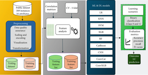
This section delineates the details of the dataset accessible to the public, including the procedure of gathering data and a thorough overview of the dataset. Moreover, it highlights the techniques utilized in developing and refining the proposed LC prediction model. It offers an in-depth explanation of each model and ends with examining their performance metrics. Furthermore, it presents the comprehensive structure of the proposed framework for the detection of LC, as illustrated in Figure 1.
3.1. Experimental Setup
The experimental setup was conducted on a high-performance computing workstation equipped with an Intel Core i7-11800h processor running at 2.30 GHz, 32 GB DDR4 RAM, and an NVIDIA GeForce RTX 3060 GPU with 6 GB of dedicated memory, operating on Windows 11 Professional 64-bit. All experiments were implemented using Python 3.10 as the primary programming environment. DL models, including the lightweight 1D CNN used for feature extraction, were developed using Tensor Flow 2.11 and Keras libraries. Traditional ML models such as logistic regression (LR), KNN, SVM, RF, XGBoost, and CatBoost were implemented using the Scikit-learn, XGBoost, and CatBoost libraries. Data preprocessing, augmentation, and visualization were performed using Pandas, NumPy, Matplotlib, and Seaborn libraries [62]. The setup leveraged the computing power of the workstation to handle the complex tasks of training DL models and evaluating performance metrics.
3.1.1. Handling of Missing Values
Before building the predictive models, we thoroughly examined the dataset for any missing entries. While key features such as age, smoking status, and fatigue were complete, a few other attributes contained missing values in the datasets. To preserve the dataset and avoid discarding potentially useful samples, we applied straightforward imputation techniques for any missing values in the datasets. For numerical features, missing values were replaced with the mean of the respective column. For categorical features, the most frequent value (mode) was used. This approach maintained the consistency and size of the dataset without introducing bias from row deletion. All data preprocessing steps, including missing value handling, were performed using Python libraries such as Pandas and Scikit-learn.
3.2. Dataset
A publicly available dataset (https://www.kaggle.com/datasets/mysarahmadbhat/lung-cancer) was utilized for this study [63]. The dataset involved a survey conducted among individuals with and without LC, aiming to investigate various characteristics that could be correlated with the illness. The dataset comprises 309 instances with 15 clinical attributes (gender, age, smoking, yellow fingers, anxiety, peer pressure, chronic disease, fatigue, allergy, wheezing, alcohol consumption, coughing, shortness of breath, swallowing difficulty, and chest pain) and one target variable (LC) [4]. To address the imbalanced class distribution between LC and non-LC instances in the dataset, SMOTE is applied [64]. Non-null counts indicate the number of available values per column, with most features being integers. However, gender and LC are categorical or textual type objects. This detailed description encapsulates preprocessed patient information or data for further processing within an ML pipeline.
3.3. ML Classifiers
In the diagnosis of LC, ML models play a pivotal role. This study employs a range of classifiers, including LR, KNN, SVM, RF, XGBoost, and CatBoost. Additionally, this work involves developing ensemble models called ConvXGB and ConvCatBoost which integrates CNN with XGBoost and CatBoost algorithms. All algorithms trained meticulously to leverage its unique strengths, aiming to deliver precise LC prognosis. To enhance model robustness, k-fold cross-validation with k = 5 was utilized, ensuring reliable performance assessment and minimizing overfitting [65]. The next section addressed the overall methods addressed in the following section.
3.3.1. LR
3.3.2. KNN
3.3.3. SVM
In the context of LC detection using SVM, the mathematical equation revolves around finding the optimal boundary that separates patients with LC from those without based on their features. Here is how the equation translates into this context:
If wT x + b > 0, the patient is classified as having LC.
If wT x + b < 0, the patient is classified as not having LC.
During training, SVM aims to find the optimal w and b values by maximizing the margin between the classes while minimizing misclassifications. These optimization processes were conducted by solving a convex optimization problem. Additionally, SVM can handle nonlinear decision boundaries by using kernel functions, which map the input features into a higher dimensional space where linear separation is possible [72].
3.3.4. XGBoost
3.3.5. RF
RF classifier serves as a potent tool for detecting and predicting the presence of LC. RF classifier evaluates the predictions of each decision tree in the forest. It selects the class label with the highest number of votes as the final prediction for the presence or absence of LC for a given patient. RF classifier in LC analysis demonstrates notable advantages, including its ability to manage noisy and unbalanced data, represent data without reduction, analyze large datasets efficiently, achieve high accuracy, and effectively address overfitting issues. These attributes make the RF classifier a reliable and resilient LC detection and prediction algorithm. These characteristics establish the RF classifier as a resilient and dependable algorithm [54]. For the mathematically inclined, the RF classifier aggregates multiple decision trees, each of which independently predicts the likelihood of a patient having LC based on a set of features or risk factors.
3.3.6. CatBoost
In this equation, L (y, p(x)) represents the loss function, where y is the true label (one for presence of LC, zero for absence) and p(x) is the model’s predicted probability that a patient has LC based on their features (x). N is the total number of patients in the dataset, and log denotes the natural logarithm. The loss function penalizes the model more heavily when its predicted probability diverges from the actual label, encouraging the model to make more accurate predictions [77]. This equation captures the essence of CatBoost optimizes the model parameters to achieve accurate predictions for binary classification tasks like LC detection.
3.4. CNN Architecture
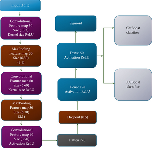
CNN [78] is a computational model that integrates convolution, pooling, and fully connected layers. The convolution and max-pooling layers’ extract features crucial for analysis, while the fully connected layers map these features to the final output. Our investigation involved implementing a 1D CNN architecture design for experimental analysis consisting of a sequence of three Conv1D layers followed by two max-pooling layers for downsampling. This CNN architecture is customized to effectively manage one-dimensional data, thus rendering it suitable for a variety of classification tasks. The architecture of this CNN [78] used in our work shows a summary of the provided CNN model (Table 1).
| Input | Layer | Feature map | Size | Kernel size | Activation |
|---|---|---|---|---|---|
| (15, 1) | Convolutional | 30 | (13, 30) | (3, 1) | ReLU |
| (13, 30) | Max pooling | 30 | (6, 30) | (2, 1) | — |
| (6, 30) | Convolutional | 60 | (6, 60) | (3, 1) | ReLU |
| (6, 60) | Max pooling | 60 | (3, 60) | (2, 1) | — |
| (3, 60) | Convolutional | 90 | (3, 90) | (3, 1) | ReLU |
| (3, 90) | Flatten | 1 | 270 | — | — |
| 270 | Dropout (0.5) | — | — | — | — |
| 270 | Dense | 128 | — | — | ReLU |
| 128 | Dense | 50 | — | — | ReLU |
| 50 | Dense | 1 | — | — | Sigmoid |
Our work introduced a CNN model with an input shape of (15, 1), representing 15 time steps and a single feature (channel). It employs three convolutional layers, with 30, 60, and 90 filters, respectively. Each filter operates with a kernel size of (3, 1), extracting features from the input data. In order to introduce nonlinearity in the network, ReLU activation functions throughout all layers were employed. Following the convolutional layers, the study applied two max-pooling layers of size (2,1) and formed new feature maps with reduced spatial dimensions when only the highest values from each region were retained. Then, a flatten layer is used to map the multidimensional feature maps to a one-dimensional vector to fit to subsequent fully connected layers. To avoid overfitting while training, a dropout layer with a 0.5 dropout rate was added. This technique randomly deactivates half of the neurons in each training step, which encourages better generalization. The network then moves to two dense layers with 128 and 50 neurons, both layers being followed by ReLU activation for enhancement of learning capacity. Finally, the output layer is a neuron with a sigmoid activation function whose output represents a probability score for the binary classification predicting LC or not in the patient. The CNN model, trained with binary cross-entropy loss, well suited for two-class problems, used Adam for optimization. The model performance with accuracy as the vital parameter was assessed. Creative design of our CNN architecture was meant to take care of 1D sequential data like the time series and structured clinical record data, which made it suitable for healthcare prediction tasks.
3.4.1. Parameters Used in the Proposed Work
In the development of the proposed ConvXGB and ConvCatBoost models, careful selection of parameters was crucial to optimize performance while maintaining computational efficiency. A lightweight 1D CNN architecture was designed with three convolutional layers, having 30, 60, and 90 filters, respectively. A small kernel size of (3,1) was chosen to capture fine-grained feature patterns across the clinical attributes, while minimizing overfitting. ReLU activation functions applied to introduce nonlinearity, enhancing the model’s ability to learn complex relationships. Pooling layers with a size of (2,1) were incorporated after convolution layers to progressively reduce the feature map dimensions and computational load, without significant loss of important information. A dropout layer with a dropout rate of 0.5 was utilized to prevent overfitting by randomly deactivating neurons during training. Fully connected dense layers of size 128 and 50 were included before the output layer to perform feature consolidation and high-level reasoning. Training of the CNN performed over 150 epochs with a batch size of 160, based on empirical testing to balance learning efficiency and convergence speed. The Adam optimizer was selected for its adaptive learning rate properties, allowing stable and faster convergence [79].
Additionally, a binary cross-entropy loss function was employed, appropriate for the binary classification nature of LC diagnosis (LC-Yes or LC-No). For the XGBoost and CatBoost classifiers, default learning rates and depth parameters were initially adopted, followed by fine-tuning based on validation performance to maximize predictive accuracy without overfitting. The choice of SMOTE for class balancing was made after observing severe imbalance in the original dataset, which could otherwise bias the model toward the majority class [80]. Finally, fivefold cross-validation was implemented to ensure a reliable and unbiased estimate of model generalization capability. The parameter choices were guided by previous best practices in similar research and by extensive experimental validation, ensuring the final models achieved optimal performance while maintaining generalizability and computational efficiency [81].
3.5. ConvCatBoost
ConvCatBoost is a novel approach that combines CNN with the CatBoost algorithm to enhance classification performance, particularly in LC detection. This fusion leverages CNN’s ability to extract intricate features from input data, while CatBoost refines predictions through gradient-boosted decision trees [82]. By integrating these two methodologies, ConvCatBoost is well-equipped to manage numerical and categorical data effectively. The resulting model exhibits improved accuracy and robustness, making it a valuable tool for early LC detection.
3.6. ConvXGB
An ensemble learning based ConvXGB algorithm is proposed to address classification challenges for LC detection effectively. ConvXGB combines the functionalities of CNN [83] and XGBoost [73], thereby leveraging the strengths inherent in both methodologies. ConvXGB encompasses two fundamental components, aiming to synergistically merge the capabilities of CNN [83] and XGBoost [84]. Employing CNN for feature extraction effectively captures important spatial patterns essential for identifying LC. Pretrained CNN models are employed to extract features, which are fed into an ensemble part for classification. After extracting features, ConvXGB leverages the XGBoost component to analyze the data, iteratively refining predictions. By combining these refined predictions, ConvXGB provides accurate diagnoses of LC, reflecting the probability of its presence based on both input data and extracted features. The detailed steps of this process are outlined (Algorithm 1), which defines the pseudocode for the ConvXGB model algorithm.
-
Algorithm 1: Pseudocode of the ConvXGB.
-
Input: Experimental dataset D
-
Parameters: Number of epochs N, feature vector dimension k, learning rate, optimizer settings
-
1. Initialize CNN model C
-
2. Initialize XGBoost classifier XGB
-
3. Apply SMOTE to dataset D to balance class distribution
-
4. Split D into training set Dtrain (90%) and validation set Dval (10%)
-
5. For each epoch =1= 1 to N do
-
6. Train CNN model C:
-
Input: Xtrain
-
Output: Deep feature vectors z∈ℝk from the penultimate Dense layer
-
Loss: Binary Cross-Entropy
-
-
Optimizer: Adam
-
7. Validate CNN model on Dval
-
8. End For
-
9. Extract deep features:
-
10. Ztrain=C(Xtrain), Zval=C(Xval)
-
11. Train XGBoost model XGBoost:
-
12. Input: Ztrain, Labels: Ytrain
-
13. Objective:
-
Obj=
-
where L is binary logistic loss, Ω is regularization
-
14. Predict on validation features Zval: Output: ŷval
-
15. Evaluate model on Dval:
-
Accuracy = TP + TN/TP + TN + FP + FN
-
Precision = TP/TP + FP
-
Recall = TP/TP + FN
-
F1 − Score = 2 × Precision × Recall/Precision + Recall
-
AUC = Area under ROC curve
-
16. Return: Predicted LC classes (LC-Yes/LC-No)
-
Output: Predicted lung cancer classes (LC-Yes/LC-No)
3.6.1. Rationalization for Employing Ensemble Models
Three ensemble models—CNN [85, 86], ConvCatBoost, and ConvXGB—apply together because they leverage deep feature learning capabilities while bringing robustness to tabular data classification. DL models called CNNs provide optimal capability to detect nonlinear patterns within medical data derived from structured clinical records [87]. CNNs demonstrate disadvantages regarding interpretability along with overfitting problems that occur when working with small or unbalanced medical datasets. XGBoost and CatBoost demonstrate high effectiveness in structured data processing while delivering good generalization through iterative weak learner aggregation and enhanced management of unbalanced datasets [88]. The ensemble method connects XGBoost and CatBoost classifiers to CNN-based deep feature extraction to gain the hierarchical learning advantages of CNN and ensemble boosting methods’ strong predictive performance with regularization properties [89]. The proposed ensemble combination addresses separate model weaknesses and produces better diagnostic accuracy while solving overfitting problems and achieving superior performance with unbalanced datasets, which are fundamental for LC detection needs [90]. The empirical analysis shows that ConvXGB and ConvCatBoost perform better than traditional ML algorithms and standalone CNN models when measuring all important performance indicators, thus supporting the successful implementation of proposed ensemble approach [61].
3.6.2. Integration of CNN Features With CatBoost and XGBoost
The decision to develop ensemble models ConvXGB and ConvCatBoost was driven by the need to integrate the strengths of both DL and gradient boosting approaches for robust LC prediction. CNNs are well-suited for capturing hierarchical and nonlinear patterns within structured data, but they are prone to overfitting when trained on small or imbalanced clinical datasets and often lack interpretability. In contrast, XGBoost and CatBoost are gradient boosting algorithms that excel in processing tabular data, offer superior regularization capabilities, and are highly effective in handling class imbalance—a common issue in medical datasets. By first extracting deep features using a lightweight 1D CNN and then passing those high-level representations into XGBoost and CatBoost classifiers, the ensemble models harness both local feature learning and strong predictive generalization. This architecture was specifically selected after comparative evaluations demonstrated that these combinations consistently outperformed standalone CNN, XGBoost, CatBoost, and traditional ML models across all key performance metrics. Thus, the ensemble strategy not only enhances classification performance but also ensures robustness, scalability, and clinical interpretability—all critical factors for real-world LC diagnostic applications.
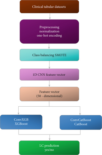
The method uses CNN features through a structured two-stage ensemble model which incorporates CatBoost along with XGBoost. A preprocessing step normalizes clinical tabular features through min–max normalization and one-hot encoding of categorical data. This process applies to the dataset which contains 309 samples and 15 features. The class unbalance is solved through the SMOTE that produces an equalized dataset for training purposes. A 1D CNN operates as a lightweight extractor for high-level features during the second processing stage. The designed CNN uses three Conv1D layers with ReLU activation functions followed by two MaxPooling1D layers alongside two dense layers with 128 neurons and 50 neurons, respectively. Training of the CNN model occurs through 150 epochs with 160 batch size using the binary cross-entropy loss function and the Adam optimizer [91]. The trained deep feature vectors consist of 50 dimensions extracted from the second-last dense layer, which produces a feature matrix with a shape of (309, 50) [92]. The extracted features provide input to independently train two boosting algorithms known as ConvCatBoost operated by CatBoost and the ConvXGB system built using XGBoost. CatBoost adopts a logistic loss for its optimization process. The CNN trains separately from both boosting models, which execute the last stage of binary cancer classification [93]. The analysis uses a fivefold cross-validation technique throughout CNN feature extraction and training of two boosting classifiers (CatBoost and XGBoost) to achieve a consistent, robust, and unbiased assessment. These boosting models from ConvCatBoost and ConvXGB generate two-class predictions for LC-Yes or LC-No, which receive their performance evaluation metrics. The two-stage ensemble methodology lets CNN extract complicated patterns from data before gradient boosting algorithms use them to improve clinical decisions, thus forming a practical framework for detecting LC.
- •
Data preprocessing: The raw clinical dataset (309 samples × 15 features) is normalized using min–max scaling, and categorical variables (e.g., gender and LC status) are encoded using one-hot encoding.
- •
Balancing classes: SMOTE is applied to handle class imbalance, resulting in a balanced dataset (550 samples).
- •
CNN-based feature extraction:
- •
A lightweight 1D CNN is trained on the structured tabular data. The architecture includes three convolutional layers followed by max-pooling layers, dropout, and dense layers.
- •
Deep features are extracted from the penultimate dense layer (128 or 50 dimensions depending on configuration), resulting in a feature matrix of shape (N, D), where N is the number of samples and D is the feature vector size (e.g., 50).
- •
- •
Ensemble learning stage:
- ➢
The extracted features are fed into two separate classifiers:
- ▪
ConvXGB: uses XGBoost for final classification.
- ▪
ConvCatBoost: uses CatBoost for final classification.
- ▪
- ➢
Both classifiers are trained on the CNN-generated feature vectors using binary logistic loss.
- ➢
- •
Model evaluation:
- •
Fivefold cross-validation is applied.
- •
Metrics such as accuracy, precision, recall, F1-score, and AUC are computed.
- •
This modular pipeline ensures that CNN handles deep pattern extraction, while boosting classifiers focus on robust, interpretable decision boundaries. A visual overview is provided in Figures 2 and 3. The process includes data preprocessing, class balancing using SMOTE, CNN-based feature extraction, and classification using gradient boosting models (XGBoost and CatBoost) in Figure 3.
The ensemble models ConvXGB and ConvCatBoost were chosen to exploit the complementary strengths of CNNs and gradient boosting techniques (XGBoost and CatBoost). CNNs excel at hierarchical feature extraction, especially in handling nonlinear patterns from structured or spatial data. However, they may struggle with small or imbalanced datasets and lack interpretability. On the other hand, XGBoost and CatBoost are highly efficient with structured clinical/tabular data, offer strong regularization, and are particularly effective in managing class imbalance, which is common in medical datasets. By combining CNN for deep feature extraction with CatBoost and XGBoost for robust classification, we aim to create an ensemble architecture that mitigates individual weaknesses (like CNN overfitting or limited tabular performance) and boosts classification accuracy, precision, and recall, especially in early-stage LC detection. These specific ensemble models were selected after a comparative evaluation of multiple classifiers, showing consistent improvement across performance metrics over both standalone CNN and traditional ML models.
3.7. Performance Evaluations Method
These performances were assessed using the confusion matrix, which comprises TP, true negative (TN), FP, and FN elements.
In our study, model performance is assessed using standard classification metrics including accuracy, precision, recall, F1-score, and area under the receiver operating characteristic curve (AUC-ROC). The confusion matrices presented in figures are based on results from individual validation folds or single 90:10 train-validation splits and reflect model performance at a fixed decision threshold of 0.5 [96]. In contrast, the AUC values reported in summary tables are calculated from ROC curves that consider all possible classification thresholds, providing a threshold-independent evaluation of model performance. Furthermore, AUC results are averaged over fivefold cross-validation to ensure robustness and generalizability [97]. This distinction explains the differences observed between confusion matrix–based estimations and AUC scores in the results.
4. Results and Discussion
Our results outline robust preprocessing, diverse feature analysis, and rigorous evaluation of ML models for LC detection. Overall, XGBoost excelled in accuracy and AUC, with SMOTE enhancing model performance. Confusion matrices and ROC curves illustrated model efficacy before and after dataset balancing. CNN and ensemble models used in the detection of LC demonstrated promise, underscoring the necessity of mitigating class unbalance in medical datasets to ensure accurate predictions and diagnosis, thus advancing patient care and disease management in healthcare analytics.
4.1. Data Preprocessing and Dataset Preparation
The initial steps in detecting LC involve preprocessing the dataset to address outliers and remove unnecessary information, ensuring data quality and reliability. Dealing with missing values is crucial, and various ML techniques are employed to address this issue by enhancing dataset quality. Training aims to optimize model parameters for accurate LC detection, while testing addresses the validation of the model in generalizing performance over new data instances.
Prior to the analysis, the dataset was preprocessed to ensure proper scaling and encoding of the variables. Continuous features, such as age, are scaled using min–max normalization to transform the values to a common range between 0 and 1. Then categorical variables, such as gender and LC status, were encoded using one-hot encoding. This technique transforms each categorical variable into a set of binary values, where each column represents a unique category.
- •
Normalization: Continuous variables were rescaled using min–max normalization to a [0,1] range.
- •
Encoding: Categorical variables were converted into numerical format through one-hot encoding.
- •
Class balancing: SMOTE is applied to synthetically augment the minority class samples, addressing the unbalance between LC-positive and LC-negative cases.
A detailed overview of the dataset partitioning, both before and after applying SMOTE, is summarized in Table 2. The dataset was split into training and validation sets using a 90:10 ratio.
| Dataset version | Training samples | Validation samples | Total samples |
|---|---|---|---|
| Original dataset | 278 | 31 | 309 |
| SMOTE-balanced dataset | 500 | 50 | 550 |
4.2. Feature Extraction
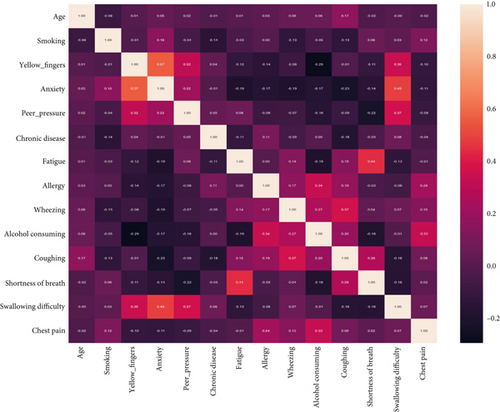
Feature analysis in the study utilized an extensive array of variables to encompass the complex aspects of LC. These variables encompassed factors like smoking history, cough presence, alcohol consumption, and yellow finger appearance. The correlation matrix and heat map visualizations were utilized to identify trends and associations among the distinct characteristics in the dataset. This thorough feature engineering process aimed to capture the most relevant and informative predictors of LC.
The representation of features in each class is shown in Table 3. Regarding gender, both males and females demonstrate comparable probabilities of receiving an LC diagnosis. Our examination indicates that each scrutinized feature is detectable in LC patients to varying degrees, spanning from 25% to 36%. Moreover, a noteworthy portion of individuals displays these symptoms even in the absence of an LC diagnosis. Regular clinical assessments and monitoring of risk factors may assist in averting or alleviating the detrimental consequences of LC, notwithstanding the absence of the disease.
| Features | LC | Features | LC | ||
|---|---|---|---|---|---|
| Gender | No | Yew | Allergy | No | Yes |
| Female | 7.485 | 42.515 | No | 12.410 | 37.590 |
| Male | 5.245 | 44.755 | Yes | 1.455 | 48.545 |
| Smoking | No | Yes | Wheezing | No | Yes |
| No | 7.405 | 42.595 | No | 10.950 | 39.050 |
| Yes | 5.460 | 44.540 | Yes | 2.615 | 47.385 |
| Yellow fingers | No | Yes | Alcohol consuming | No | Yes |
| No | 9.775 | 40.225 | No | 11.680 | 38.320 |
| Yes | 3.695 | 46.305 | Yes | 2.035 | 47.965 |
| Anxiety | No | Yes | Coughing | No | Yes |
| No | 8.710 | 41.290 | No | 11.155 | 38.845 |
| Yes | 3.895 | 46.105 | Yes | 2.795 | 47.205 |
| Peer pressure | No | Yes | Shortness of breath | No | Yes |
| No | 9.415 | 40.585 | No | 7.660 | 42.340 |
| Yes | 3.225 | 46.775 | Yes | 5.555 | 44.445 |
| Chronic disease | No | Yes | Swallowing difficulty | No | Yes |
| No | 8.170 | 41.830 | No | 10.365 | 39.635 |
| Yes | 4.485 | 45.515 | Yes | 1.725 | 48.275 |
| Fatigue | No | Yes | Chest pain | No | Yes |
| No | 9.900 | 40.100 | No | 9.855 | 40.145 |
| Yes | 4.565 | 45.435 | Yes | 3.490 | 46.510 |
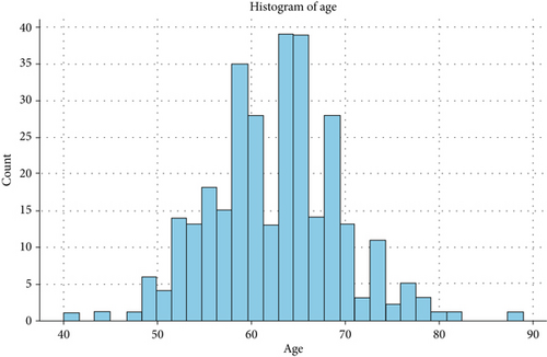
Figure 4 illustrates the distribution of participants across different age groups, revealing a higher prevalence of LC among individuals aged 50–79. Among these age groups, the 60–64 age bracket exhibits the highest frequency of LC cases. The relationships between features based on the heat map mentioned in Figure 5 were designed.
4.3. Performance Evaluation of LC Prediction Based on Unbalanced Data Using ML
To predict LC, ML algorithms such as LR, KNN, SVM, XGBoost, RF, and CatBoost with cross-validation folds such as 1, 2, 3, 4, and 5 techniques (Table 4) were used. Additionally, we employed SMOTE to balance the data. It was found that in the case of an unbalanced dataset, the RF model has the highest performance in terms of accuracy, recall, AUC, F1-score, and precision, which were found to be 0.7201, 0.9748, 0.9356, 0.9484, and 0.9198, respectively. Additionally, the mean KNN model of this study has the lowest performance in terms of accuracy, recall, AUC, F1-score, and precision, which were found to be 0.6648, 0.9680, 0.8532, 0.9347, and 0.9074, respectively.
| Model | Fold | Accuracy | Recall | AUC | F1-score | Precision |
|---|---|---|---|---|---|---|
| LR | 1 | 0.7416 | 0.9833 | 0.9416 | 0.9833 | 0.9833 |
| 2 | 0.7683 | 0.9811 | 0.9601 | 0.9541 | 0.9285 | |
| 3 | 0.6870 | 0.9454 | 0.9194 | 0.9369 | 0.9285 | |
| 4 | 0.6000 | 1.0000 | 0.9815 | 0.8867 | 0.7966 | |
| 5 | 0.7227 | 0.9454 | 0.9181 | 0.9454 | 0.9454 | |
| Mean | 0.7039 | 0.9636 | 0.9442 | 0.9413 | 0.9165 | |
| KNN | 1 | 0.725 | 0.950 | 0.7000 | 0.9661 | 0.9827 |
| 2 | 0.7683 | 0.9811 | 0.9098 | 0.9541 | 0.9285 | |
| 3 | 0.6246 | 0.9636 | 0.8467 | 0.9380 | 0.9137 | |
| 4 | 0.5666 | 1.0000 | 0.9730 | 0.8785 | 0.7833 | |
| 5 | 0.6393 | 0.9454 | 0.8363 | 0.9369 | 0.9285 | |
| Mean | 0.6648 | 0.9680 | 0.8532 | 0.9347 | 0.9074 | |
| SVM | 1 | 0.7333 | 0.9666 | 0.9750 | 0.9747 | 0.9830 |
| 2 | 0.7127 | 0.9811 | 0.9329 | 0.9454 | 0.9122 | |
| 3 | 0.7675 | 0.9636 | 0.8987 | 0.9549 | 0.9464 | |
| 4 | 0.5666 | 1.000 | 0.9673 | 0.8785 | 0.7833 | |
| 5 | 0.8060 | 0.9454 | 0.8969 | 0.9541 | 0.9629 | |
| Mean | 0.7172 | 0.9713 | 0.9341 | 0.9415 | 0.9176 | |
| XGBoost | 1 | 0.7500 | 1.0000 | 0.9500 | 0.9915 | 0.9836 |
| 2 | 0.5922 | 0.9622 | 0.8322 | 0.9189 | 0.8793 | |
| 3 | 0.7493 | 0.9272 | 0.8207 | 0.9357 | 0.9444 | |
| 4 | 0.6333 | 1.0000 | 0.9801 | 0.8952 | 0.8103 | |
| 5 | 0.7878 | 0.9090 | 0.9424 | 0.9345 | 0.9615 | |
| Mean | 0.7025 | 0.9597 | 0.9051 | 0.9352 | 0.9158 | |
| RF | 1 | 0.7416 | 0.9833 | 0.9333 | 0.9833 | 0.9833 |
| 2 | 0.7777 | 1.0000 | 0.9643 | 0.9724 | 0.9285 | |
| 3 | 0.7675 | 0.9636 | 0.8792 | 0.9549 | 0.9464 | |
| 4 | 0.6000 | 1.0000 | 0.9574 | 0.8867 | 0.7966 | |
| 5 | 0.7136 | 0.9272 | 0.9606 | 0.9444 | 0.9444 | |
| Mean | 0.7201 | 0.9748 | 0.9389 | 0.9484 | 0.9198 | |
| CatBoost | 1 | 0.7416 | 0.9833 | 0.9000 | 0.9833 | 0.9833 |
| 2 | 0.6667 | 1.0000 | 0.9433 | 0.9464 | 0.8983 | |
| 3 | 0.7675 | 0.9636 | 0.8831 | 0.9549 | 0.9464 | |
| 4 | 0.6000 | 1.0000 | 0.9730 | 0.8867 | 0.7966 | |
| 5 | 0.7136 | 0.9272 | 0.9424 | 0.9357 | 0.9444 | |
| Mean | 0.6979 | 0.9748 | 0.9283 | 0.9414 | 0.9138 | |
- Note: Bold data means maximum value.
4.4. Performance Evaluation of LC Prediction Based on Balanced Data Using ML
The LR, KNN, SVM, XGBoost, RF, and CatBoost models with fivefold cross-validation techniques are used to predict LC based on balanced data (Table 5). The low precision (0.100) for the CNN model may be due to a high number of FPs in the balanced dataset, potentially caused by insufficient feature discrimination in the standalone CNN architecture. To mitigate overfitting observed in the CNN model, a dropout rate of 0.5 was applied, and early stopping techniques were explored, which showed potential for improving generalization on the balanced dataset. It was found that the CatBoost model of this study has the highest performance in terms of accuracy, recall, AUC, F1-score, and precision, which were found to be 0.9550, 0.9398, 0.9895, 0.9541, and 0.9708, respectively, under the balance dataset. Additionally, the mean KNN model of this study has the lowest performance in terms of accuracy, recall, AUC, and F1-score, which are found to be 0.9143, 0.8286, 0.9635, and 0.9056, respectively. While the lowest precision is 0.9346 for the LR model.
| Model | Fold | Accuracy | Recall | AUC | F1-score | Precision |
|---|---|---|---|---|---|---|
| LR | 1 | 0.8993 | 0.8776 | 0.9810 | 0.9009 | 0.9259 |
| 2 | 0.9168 | 0.9107 | 0.9890 | 0.9189 | 0.9272 | |
| 3 | 0.8880 | 0.8653 | 0.9361 | 0.8832 | 0.9000 | |
| 4 | 0.9440 | 0.9245 | 0.9735 | 0.9423 | 0.9607 | |
| 5 | 0.9340 | 0.9038 | 0.9478 | 0.9306 | 0.9591 | |
| Mean | 0.9164 | 0.8963 | 0.9863 | 0.9150 | 0.9346 | |
| KNN | 1 | 0.9473 | 0.8947 | 0.9836 | 0.9444 | 0.9807 |
| 2 | 0.9017 | 0.8035 | 0.9656 | 0.8910 | 1.0000 | |
| 3 | 0.8846 | 0.7692 | 0.9416 | 0.8695 | 1.0000 | |
| 4 | 0.9339 | 0.8679 | 0.9636 | 0.9292 | 1.0000 | |
| 5 | 0.9038 | 0.8076 | 0.9635 | 0.8936 | 0.9767 | |
| Mean | 0.9143 | 0.8286 | 0.9635 | 0.9056 | 0.9915 | |
| SVM | 1 | 0.9649 | 0.9298 | 0.9858 | 0.9636 | 1.0000 |
| 2 | 0.9361 | 0.9107 | 0.9934 | 0.9357 | 0.9622 | |
| 3 | 0.9038 | 0.8076 | 0.9845 | 0.8936 | 1.0000 | |
| 4 | 0.9535 | 0.9433 | 0.9910 | 0.9523 | 0.9615 | |
| 5 | 0.9615 | 0.9230 | 0.9663 | 0.9600 | 1.0000 | |
| Mean | 0.9439 | 0.9029 | 0.9843 | 0.9410 | 0.9847 | |
| XGBoost | 1 | 0.9705 | 1.0000 | 0.9962 | 0.9743 | 0.9500 |
| 2 | 0.9532 | 0.9642 | 0.9842 | 0.9557 | 0.9473 | |
| 3 | 0.9237 | 0.8653 | 0.9649 | 0.9183 | 0.9782 | |
| 4 | 0.9538 | 0.9694 | 0.9828 | 0.9532 | 0.9444 | |
| 5 | 0.9711 | 0.9828 | 0.9752 | 0.9702 | 1.0000 | |
| Mean | 0.9545 | 0.9468 | 0.9817 | 0.9544 | 0.9640 | |
| RF | 1 | 0.9520 | 0.9824 | 0.9951 | 0.9739 | 0.9655 |
| 2 | 0.9622 | 0.9821 | 0.9953 | 0.9565 | 0.9482 | |
| 3 | 0.9423 | 0.8846 | 0.9908 | 0.9292 | 1.0000 | |
| 4 | 0.9447 | 0.9622 | 0.9902 | 0.9444 | 0.9272 | |
| 5 | 0.9711 | 0.9423 | 0.9934 | 0.9607 | 1.0000 | |
| Mean | 0.9544 | 0.9507 | 0.9930 | 0.9529 | 0.9682 | |
| CatBoost | 1 | 0.9628 | 0.9649 | 0.9979 | 0.9649 | 0.9649 |
| 2 | 0.9725 | 0.9642 | 0.9965 | 0.9729 | 0.9818 | |
| 3 | 0.9326 | 0.8653 | 0.9910 | 0.9278 | 1.0000 | |
| 4 | 0.9447 | 0.9622 | 0.9790 | 0.9444 | 0.9272 | |
| 5 | 0.9622 | 0.9423 | 0.9831 | 0.9602 | 0.9800 | |
| Mean | 0.9550 | 0.9398 | 0.9895 | 0.9541 | 0.9708 | |
- Note: Bold data means maximum value.
4.5. Performance Evaluation of LC Prediction Based on Unbalanced Data Using CNN and Ensemble DL Models
In this section, the performance of the proposed CNN and ensemble approach is evaluated for the unbalanced dataset. To train CNN with the unbalanced dataset, it is divided into training and validation sets as 90:10, respectively. In this phase, the proposed CNN architecture facilitates simultaneous training and testing of models. With 150 epochs configured and a batch size of 160, the model iterates through the dataset, honing its understanding of the features within. The validation loss and accuracy curve for CNN across different epochs for the unbalanced dataset is shown in Figure 6.
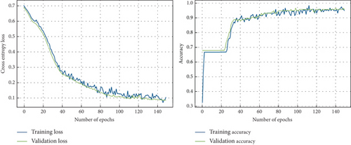
Overall proposed CNN model learned with low bias, and the model seems to be overfitting, followed by less learning till 25 epochs; then, the model showed improved learning. In this work, an ensemble-based approach in composition of the CNN model with XGBoost and CatBoost classifiers based on their performance demonstrated (Tables 4 and 6) is proposed. Deep features are fed to ensemble learning models, namely, ConvCatBoost and ConvXGB, for the prediction of LC.
| Metric | CNN | ConvCatBoost | ConvXGB |
|---|---|---|---|
| Accuracy | 0.9565 | 0.9736 | 0.9739 |
| Precision | 0.9740 | 0.9870 | 0.9747 |
| Recall | 0.9615 | 0.9744 | 0.9872 |
| F1-score | 0.9677 | 0.9806 | 0.9803 |
The performance of CNN models of this study is evaluated under unbalanced dataset using confusion matrices and ROC curves as shown in Figures 7 and 8, respectively. The confusion matrix provides overall performance metrics for the CNN and deep ensemble models ConvCatBoost and ConvXGB by comparing predicted and true labels for LC prediction. The CNN model’s metrics such as accuracy (0.9565), precision (0.9740), recall (0.9615), and F1-score (0.9677) highlight its effectiveness in binary classification tasks.
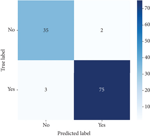
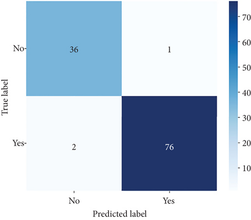
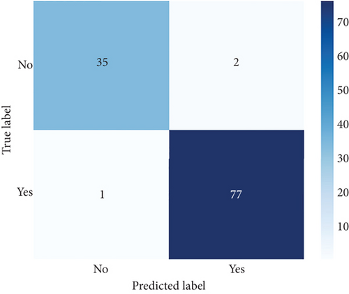
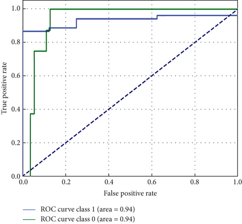
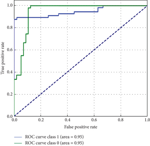
Overall, Figure 7 indicates that ConvXGB demonstrated superior performance compared to CNN and ConvCatBoost, particularly regarding FP and TN for predicting LC. The ROC curve in Figure 8 for CNN and ensemble models ConvCatBoost and ConvXGB using unbalanced dataset illustrates binary classification performance across various threshold settings. It plots the TPR against the FPR, offering insight into the trade-offs between precision and recall. The ensemble models outperformed the baseline CNN model in terms of the ROC curve.
The performance of the CNN and ensemble-based models, namely, ConvXGB and ConvCatBoost, was evaluated for LC prediction on the unbalanced dataset. Performance metrics such as accuracy, precision, recall, and F1-score were derived from the confusion matrix for all models. The results for CNN, ConvCatBoost, and ConvXGB (Table 6) showed that the overall LC prediction performances in terms of accuracy with the unbalanced datasets were 0.9565 for CNN, 0.9736 for ConvCatBoost, and 0.9739 for ConvXGB, respectively. Similarly, LC prediction performances in terms of precision with the unbalanced dataset were 0.9740, 0.9870, and 0.9747 for CNN, ConvCatBoost, and ConvXGB, respectively. LC prediction performances in terms of recall with the unbalanced dataset were 0.9615, 0.9744, and 0.9872 for CNN, ConvCatBoost, and ConvXGB, respectively. In terms of F1-score with the unbalanced dataset, the scores were 0.9677, 0.9806, and 0.9803 for CNN, ConvCatBoost, and ConvXGB, respectively. In the proposed work of this study, the CNN and ensemble DL models using the unbalanced data ConvCatBoost and ConvXGB exhibit superior accuracy, implying better classification despite data imbalance. While CNN and ConvCatBoost demonstrated higher precision, ConvXGB showed a slight lag in precision. Recall scores show consistency among CNN and ConvCatBoost, with ConvXGB slightly lower. ConvCatBoost tops the F1-score, followed closely by CNN and ConvXGB, indicating robust performance in LC detection despite unbalanced dataset challenges.
4.6. Performance Evaluation of LC Prediction Based on Balanced Data Using CNN and Ensemble DL Models
In this section, a performance evaluation of LC prediction using CNN and an ensemble approach for the balanced dataset was conducted. The CNN training phase comprised 150 epochs, with a batch size set to 160 for each epoch, averaging 39 ms/step. Following training, the CNNs exhibited enhanced performance in comparison to conventional ML techniques by achieving a remarkable accuracy of 95.13%. Additionally, the findings of this study are supplemented with visual representations in Figure 9, which illustrate the learning process of the CNN model on the balanced dataset.

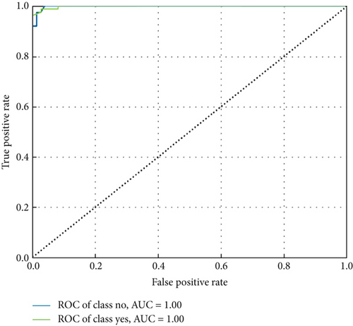
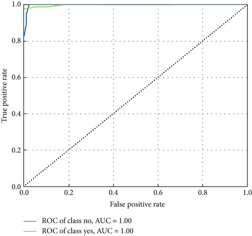
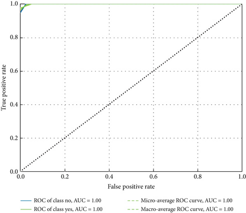
ConvCatBoost and ConvXGB, both deep ensemble models integrating CNN and boosting algorithms, were demonstrated remarkable performance in binary classification for LC prediction. ConvCatBoost shows precision (0.9870) and recall (0.9744), with accuracy (0.9736) and notable F1-scores (0.9806), indicating accurate categorization. Meanwhile, ConvXGB achieved impeccable recall (0.9872) and high precision (0.9872), resulting in an accuracy (0.9826) and impressive F1-scores (0.9872). Overall, ConvXGB outperformed with exceptional precision, recall, and F1-scores, highlighting its efficacy in precise classification tasks. Confusion matrix for balance data with deep ensemble models CNN, ConvCatBoost, and ConvXGB shown in Figure 10 described the classification task for prediction LC with predicted and true levels. Figure 11 explains the ROC curve results for the CNN with Sigmoid model, ConvCatBoost, and ConvXGB, respectively, indicating AUC is 1.00, indicating perfect discrimination between positive and negative instances.

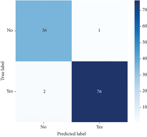
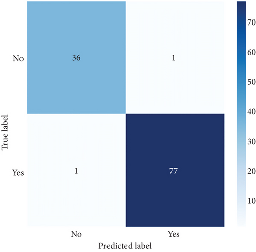

In the CNN-based ensemble model of this study, the performance for balanced data (Table 7) presents the performance measures such as accuracy, precision, recall, and F1-score for DL architectures: CNN utilizing sigmoid activation, ConvCatBoost, and ConvXGB. ConvXGB attains the highest values in accuracy (0.9826) and precision (0.9872), surpassing recall (0.9872) and F1-score (0.9872), demonstrating a robust overall performance. In comparison, ConvCatBoost demonstrates inferior performance when contrasted with ConvXGB, with values of accuracy, precision, recall, and F1-score of 0.9736, 0.9870, 0.9744, and 0.9806, respectively. The CNN model employing sigmoid activation achieves recall (0.9024), implying accurate positive forecasts, albeit with precision (0.100) and F1-score (0.487) in relation to ConvXGB. In summary, ConvXGB emerges as the most effective model across all criteria, displaying superior levels of accuracy, precision, recall, and F1-score.
| Metric | CNN | ConvCatBoost | ConvXGB |
|---|---|---|---|
| Accuracy | 0.9652 | 0.9736 | 0.9826 |
| Precision | 0.100 | 0.9870 | 0.9872 |
| Recall | 0.9024 | 0.9744 | 0.9872 |
| F1-score | 0.9487 | 0.9806 | 0.9872 |
4.7. Comparison Results Among Various LC Prediction Models
This research shows a breakdown of the models’ performance metrics, including accuracy, precision, recall, and F1-score (Table 8). An extensive assessment conducted for range of classifiers, encompassing conventional approaches like LR, KNN, SVM, XGBoost, RF, and CatBoost and DL-based CNN model, as well as ensemble methods like ConvXGB and ConvCatBoost. Overall, ConvXGB emerged as the most effective performer across evaluation metrics, displaying outstanding levels of accuracy (98.26%), recall (98.72%), and F1-score (98.72%) in contrast of precision KNN outperformed all models by exhibiting high precision (99.15%). This highlights the potency of amalgamating the representational capacity of CNN with the boosting capabilities of XGBoost for robust binary classification. CNN and ConvCatBoost also exhibited noteworthy outcomes, particularly excelling in recall and F1-score, demonstrating their adeptness in precisely recognizing positive instances. Ensemble methods such as ConvXGB and ConvCatBoost demonstrated competitive performance, attaining elevated accuracy levels and maintaining balanced precision–recall trade-offs. Traditional methods like LR, KNN, SVM, XGBoost, RF, and CatBoost also delivered respectable results, albeit with slight discrepancies in certain metrics. These discoveries give important advice to researchers and practitioners in the identification of fitting classifiers customized to demands and circumstances, hence supporting creativity and development in ML and AI research.
| Metric | LR | KNN | SVM | XGBoost | RF | CatBoost | CNN | ConvCatBoost | ConvXGB |
|---|---|---|---|---|---|---|---|---|---|
| Accuracy | 0.9146 | 0.9143 | 0.9439 | 0.9545 | 0.9544 | 0.9550 | 0.9652 | 0.9736 | 0.9826 |
| Precision | 0.9346 | 0.9915 | 0.9847 | 0.9640 | 0.9682 | 0.9708 | 0.100 | 0.9870 | 0.9872 |
| Recall | 0.8963 | 0.8286 | 0.9029 | 0.9468 | 0.9507 | 0.9398 | 0.9024 | 0.9744 | 0.9872 |
| F1-score | 0.9150 | 0.9065 | 0.9410 | 0.9544 | 0.9529 | 0.9541 | 0.9487 | 0.9806 | 0.9872 |
- Note: Bold data means maximum value.
4.8. Comparison of the Proposed and Existing Methods
In the comparison of the proposed ensemble DL models of this study with the fundamental methodology analyzed in this study to augment accuracy and efficiency (Table 9), it was demonstrated that there is a contrast with previously documented research. This study’s proposed ensemble DL model shows a significant improvement in accuracy and efficiency compared to earlier methodologies explored in this study. Past research utilizing models such as ANN, WDELM, CNN, and RotF has reported commendable accuracy levels. However, the proposed approach of this study stands out due to its ensemble design, which integrates the strengths of CNN and XGBoost. This fusion enables the model of this study to achieve impressive accuracy, outperforming previously documented models.
This high level of performance emphasizes the effectiveness of the frame worked this study in accurately classifying cases into LC-Yes and LC-No categories. By combining the feature-learning capability of CNNs with the powerful classification strength of XGBoost, the ensemble model of this study captures both spatial and structured data patterns with high precision. Moreover, the inclusion of the SMOTE addresses class imbalance, enhancing the model’s ability to generalize across diverse clinical scenarios.
LC detection remains a critical area in medical AI due to its high mortality rate and the need for early, accurate diagnosis. Over the years, researchers have explored various ML and DL techniques to improve prediction outcomes. ANN models, for example, have been widely used due to their ability to handle complex nonlinear data. One such model achieved 90.91% accuracy on a multimodal clinical dataset [99], while another study reported 93% using public medical data [19]. Despite these results, ANN performance is often highly dependent on data quality and can struggle with large, high-dimensional datasets.
Ensemble models such as WDELM have shown moderate success by combining multiple learners, achieving 92% accuracy on LC datasets [100]. While ensemble methods offer robustness, they sometimes rely on hand-crafted features or shallow models, which may not fully capture intricate patterns in medical imaging. DL architectures like CNNs have addressed this limitation by automatically learning hierarchical representations from image data, with one CNN-based model reaching 95% accuracy [101]. Additionally, RotF, an ensemble technique, achieved 97.1% accuracy on demographic data [4], highlighting the strength of model diversification.
Building on these advances, the proposed ConvXGB model of this study introduces an ensemble architecture: first, deep features are extracted using a pretrained CNN, which captures spatial dependencies in the input; then, XGBoost is applied for high-precision classification. This combination leverages the advantages of both DL and gradient-boosted decision trees, allowing the model to refine predictions and improve classification performance iteratively.
The experimental results of this study confirm the superiority of ConvXGB, which not only achieves the highest accuracy 98.26% among the compared models but also excels across other key evaluation metrics such as precision, recall, F1-score, and AUC. These findings underscore the model’s robustness, reliability, and potential for real world clinical implementation. By harnessing the complementary strengths of CNN and XGBoost, ConvXGB offers a scalable and effective solution for LC prediction one that holds promise for enhancing diagnostic accuracy and supporting early intervention in clinical settings.
4.9. Applications of the Study
The manuscript endeavors to significantly improve the precision and efficacy of LC diagnosis by applying advanced ML methods. It assesses the effectiveness of ensemble learning compared to ConvXGB for detection, specifically focusing on the complexities related to tumor compositions. By connecting the power of ensemble learning and ConvXGB, the manuscript aims to exceed the constraints of traditional diagnostic approaches. The precision of diagnostic procedures is enhanced through the classification accuracy of ensemble learning and the feature extraction capabilities of ConvXGB. The research is aimed at identifying the most effective model for classifying LC, providing valuable insights into the efficiency of ensemble learning and ConvXGB in interpreting medical images. The expected outcomes suggest the enhancement of ML algorithms for precise cancer identification. This development has the potential to revolutionize the field of diagnosis and treatment, leading to improved patient outcomes and more informed clinical decision-making. It sets the stage for improved management of LC and a decrease in mortality rates.
4.10. Limitations of the Study
The investigation presents encouraging results, yet it recognizes various constraints. Initially, the magnitude and variety of the dataset might limit the model’s applicability, necessitating more extensive and diverse datasets for thorough validation. Moreover, the uneven distribution of classes within the data may skew model performance, underscoring the importance of addressing class imbalance. Furthermore, depending solely on predefined features derived from CT scans could potentially overlook significant biomarkers. Integrating sophisticated feature selection techniques or utilizing DL for automated feature extraction could boost the models’ capacity to detect subtle patterns and enhance diagnostic precision [102]. Additionally, the selection of validation methods can significantly influence the credibility of the study. Accordingly, employing a range of validation approaches and performing external validation on distinct datasets are essential measures to ensure the reliability of the results. The translation of the models into clinical practice presents challenges, including the necessity for validation in real-world scenarios and regulatory authorization. Ensuring the interpretability of models, especially for DL models recognized for their opaque nature, is crucial for clinical acceptance. Furthermore, ethical considerations such as patient confidentiality, data protection, and algorithmic biases should be meticulously managed to safeguard patient rights and foster trust in AI-driven healthcare solutions [103]. Transparent disclosure of model performance and potential biases is critical for ethical and accountable deployment. Tackling these constraints in future research can propel the domain of LC diagnosis forward, leading to the establishment of more dependable, clinically relevant, and ethically sound ML-based methodologies [104].
4.11. Future Scope of the Study
This research successfully proves the value of combined DL with ensemble methods for detecting LC, but multiple improvement areas exist for future development. The framework requires increased availability of diverse clinical reports from various institutions to ensure effective model generalization across different demographics and medical conditions. The characteristic features of early-stage LC become more detectable by the ensemble models when using multimodal data combination approaches that merge CT scan images with genomic profiles and laboratory test results [105]. XAI techniques, specifically SHAP and LIME, will serve as top priorities for the project because they help make model predictions more understandable to healthcare professionals, thus building trust between healthcare providers and the system [106]. AutoML solutions will undergo evaluation because they help automatically design model specifications and discover optimal hyperparameters, creating efficient development processes and exceptional model results [107]. The future work endeavors to convert proposed models into functional CDSSs, which will create user-friendly real-time assistance tools for physicians in early LC detection to enhance patient health results [108].
5. Conclusions
This study contributes significantly to the enhancement of LC diagnostic protocols through the integration of sophisticated ML methodologies. By employing strategies such as SMOTE for data balancing, fivefold cross-validation for performance analysis, and CNN for binary classification in LC detection, the accuracy and dependability of diagnostic processes was elevated. Moreover, the rigorous comparative analysis of this study establishes benchmarks for evaluating the efficacy of ML models in LC diagnosis, providing a robust framework for future evaluations in both unbalanced and balanced data scenarios. Furthermore, the exploration of ensemble learning techniques in this study, including ensemble CNN, ConvCatBoost, and ConvXGB, addresses the intricacies of LC diagnosis, leading to more comprehensive and resilient diagnostic frameworks. The exceptional performance of ConvXGB underscores its potential to transform LC diagnosis, offering healthcare professionals a reliable and effective tool for timely interventions and improved patient outcomes. This research highlights the groundbreaking influence of ML in LC research, opening avenues for continued progress in oncological diagnostics and treatment strategies.
Nomenclature
-
- LC
-
- lung cancer
-
- ML
-
- machine learning
-
- DL
-
- deep learning
-
- NSCLC
-
- non–small cell lung cancer
-
- SCLC
-
- small cell lung carcinoma
-
- SBRT
-
- stereotactic body radiotherapy
-
- CNN
-
- convolutional neural network
-
- RF
-
- random forest
-
- SVM
-
- support vector machine
-
- KNN
-
- K-nearest neighbor
-
- LR
-
- logistic regression
-
- XGBoost
-
- eXtreme gradient boosting
-
- CatBoost
-
- categorical boosting
-
- SMOTE
-
- synthetic minority oversampling technique
-
- CDSS
-
- clinical decision support system
-
- ROC
-
- receiver operating characteristic
-
- AUC
-
- area under the curve
-
- ANN
-
- artificial neural network
-
- MLP
-
- multilayer perceptron
-
- WDELM
-
- weighted differential extreme learning machine
-
- RotF
-
- rotation forest
-
- ConvXGB
-
- convolutional neural network with XGBoost
-
- ConvCatBoost
-
- convolutional neural network with CatBoost
-
- ReLU
-
- rectified linear unit
Conflicts of Interest
The authors declare no conflicts of interest.
Author Contributions
M.M.A. and S.K.: conceptualization, methodology, formal analysis, software, validation, and writing—original draft. M.B.B.H.: data curation, methodology, investigation, visualization, and writing—original draft. F.A.: conceptualization, formal analysis, funding acquisition, resources, supervision, project administration, and writing—review and editing. C.C.: data curation, methodology, investigation, visualization, and writing—review and editing. M.A.B.H.: data curation, methodology, validation, investigation, and writing—review and editing. E.S. and S.P.: data curation, investigation, formal analysis, and writing—original draft. R.A. and D.P.: data curation, investigation, formal analysis, and writing—review and editing. All the authors have read and agreed to the publication.
Funding
No funding was received for this manuscript.
Acknowledgments
We would like to thank Prof. Naseem, Prof. Chandel, Prof. Ansari, and Prof. Huang for their valuable support. The authors also acknowledge Integral University, Lucknow, India, for providing the manuscript communication number (IU/R&D/2024-MCN0002892) for this study.
Open Research
Data Availability Statement
All data utilized in this study is included in this article.


