1. Introduction

Dynamic traffic assignment (DTA) models are important tools for planning and managing large-scale urban networks. Calibration of DTA models of large urban networks includes several challenges. Accurately replicating real-world traffic conditions, especially in highly congested areas, requires sophisticated models that can handle complex interactions. Many characteristics of urban networks, such as complicated intersections, short links, and route choice are challenging to model, and are factors influencing the calibration [1, 2]. Further, large urban networks involve numerous variables and parameters, making the calibration process computationally demanding [3].

The precision of congestion and delay estimates of DTA models rely heavily on correctly estimated capacity parameters. Link capacities, which describe the physical property of links, are assumed fixed in this paper if we ignore factors such as weather conditions. Link capacities in dynamic urban traffic networks are typically estimated locally for each link or assigned based on general guidelines [4]. Local estimation of link capacities requires assumptions on the fundamental diagram of each link as well as flow measurements for several traffic regimes with densities both higher and lower than the critical density. In this paper, we aim to utilize the network structure in combination with link flow measurements to perform network-wide calibration of link capacities.

Most research regarding link capacity calibration focuses on the local level instead of the network level. Local calibration is done by calibrating fundamental diagrams for individual links, or individual link types [5–7]. Other related research deals with calibration of demand, that is, origin-destination (OD) calibration, and capacity calibration simultaneously. Here, the OD matrix acts as parameters and flows are outputs. Capacities appear in the constraint part of an optimization problem which minimizes the difference between the predicted link flows obtained when the OD matrix is assigned to the network and observed link flows [8, 9]. There is very limited work focusing on quantitative analysis of capacities in urban networks as well as pure capacity calibration at the network-wide level [10].

The capacity calibration problem is very challenging, not only because of the large number of link capacities to be calibrated, but also due to the complex relation between capacities and observed traffic flows. There are many acceptable capacity values which will result in identical traffic flow output. The capacity of a given link cannot be smaller than any observed flow on this link; however, the highest observed traffic flows are likely not the real capacities of the links. One example is a link acting as a bottleneck that will equivalently reduce the flows on its downstream links within a certain time period, which means we are unable to get useful information to calibrate the capacities of those downstream links.

In this paper, we aim to find an efficient capacity calibration method which can be applied to large-scale urban transportation networks. We investigate how network-wide link capacities influence the resulting flows by using a small toy network, present a novel calibration method, and evaluate the performance of the results from this method on a large-scale network model of Stockholm, Sweden.

The proposed method, based on partial least square (PLS) regression, is evaluated for the case where MATSim, an open-source framework for implementing large-scale agent-based transport simulations, is used for assigning the travel demand to the network. The evaluation is made both with respect to the quality of the resulting capacity estimates and the computational efficiency. It is evaluated by comparing the results from the proposed method with those from the method of simultaneous perturbation stochastic approximation (SPSA).

The main contribution of this paper is a novel, network-wide, calibration method for urban network link capacities. Further, the relationship between flows and capacities in the context of urban network capacity calibration is analyzed, which could be helpful for future network-wide approaches for capacity calibration.

In the next section, we go through previous work, put forward relevant earlier published calibration methods and introduce PLS regression. Section 3 presents the method developed in this paper, which contains the following major steps: trial points generation, simulation, PLS regression and capacity updates. Section 4 describes the simulation setup for evaluation of the method and the results are presented and analyzed in Section 5. The last section concludes the paper and suggests directions for further research.

2. Literature Review

In the field of traffic model calibration, most of the research focuses on demand (OD) calibration or a combination of demand and supply calibration (i.e., joint calibration).

The joint calibration of DTA models can be categorized into two groups: (1) iterative demand–supply calibration approaches and (2) simultaneous demand-supply calibration approaches [11]. For iterative calibration methods, the O-D flows and route choices are calibrated first, and then the driver behavior parameters are calibrated. These two steps are iterated until a convergence criterion is satisfied [12–14]. For simultaneous demand-supply calibration, Balakrishna [9] proposes a formulation of an optimization problem which can jointly estimate both demand (OD flow and route choice) and supply (speed–density diagram and segment capacity) parameters. Even though capacities are included in this work, they only appear in the constraint part in formulating optimization, acting as upper bounds for flows.

In terms of pure supply calibration, most of the work concentrates on speed-density relationship calibration for individual links, or individual link types [5–7]. The available literature on network-level capacity calibration is very limited. In Lin et al. [10]; a Dantzig-Wolfe decomposition-based heuristic for capacity calibration is presented and it has also been stressed that there are many acceptable capacity values which will result in identical traffic flow output, which makes capacity calibration very challenging.

There is a lot of work concentrating on improving the efficiency and accuracy of methods applied to OD calibration problems. These problems are relevant for capacity calibration since these two types of calibration problems share many similarities.

A frequently encountered calibration method includes numerical estimation of a full Jacobian matrix [15], aiming at finding the local linear approximation between the input and output variables. The issue is that high dimensionality (e.g., number of links) in networks introduces great complexity. This classical calibration method, consisting of series of iterations in which estimation of local Jacobian matrix is computed, often faces problems with computational efficiency.

One alternative to estimating the full Jacobian matrix is the SPSA method, a method that has shown improvement in computational efficiency. It simplifies multivariate optimization problems by approximating the gradient with only a small number of measurements per iteration in which all variables vary randomly [16]. Although the SPSA method is computationally efficient, the performance regarding convergence rate and calibration accuracy deteriorates greatly when the problem dimension increases. According to previous research, the calibration errors stop decreasing at relatively high values [17]. In Lu et al. [18]; different values of algorithm parameters are tested, and adaptive step sizes are evaluated, but with limited effect in decreasing the calibration error. Some researchers investigate modifications and variations of the SPSA method to achieve higher efficiency and better robustness, such as weighted SPSA [17, 19, 20] and cluster-wise SPSA [21], which have better calibration performance compared to the traditional SPSA method.

In Zhang et al. [22] and Chong and Osorio [23]; a simulation-based optimization algorithm is presented which provides a fundamental structure of the calibration method in this paper. In this method, a simulator and a sampling strategy for collecting trial points are used to update a regression-based model constructing an approximation between inputs and outputs. This regression model is further utilized in an optimization problem minimizing the difference between observed and predicted flows [22]. There has been other work focuses on improving the efficiency of sensitivity analysis based on this method. In Osorio and Bierlaire [24]; a simulation-based optimization (SO) method which improves the efficiency of complex stochastic urban traffic simulators is presented: Trial points from previous iterations are saved and a criterion is formulated to determine the acceptance of these points in a later iteration. The weight for each trail point is formed on the inverse distance weight function [25]. This trial points selection strategy is similar to what we will use in this research.

The method proposed in this paper implements a dimensionality reduction method (PLS regression) in capacity calibration problems to reduce the computational cost. PLS regression has been broadly used in chemometrics, for example, Godoy et al. [26] and Geladi and Kowalski [27] but has to the best of our knowledge not yet been used in the area of traffic model calibration.

3. Capacity Calibration

The hypothesis in this paper is that the network structure in combination with multiple link flow observations can be used to improve link capacity estimates. From the literature review, the most popular methods for capacity estimation are based on calibration of fundamental diagrams for individual links. However, for large urban networks, it can be challenging to collect enough data to support local calibration for all links. Furthermore, due to network bottlenecks, many of the links are always in an undersaturated state, which makes it hard to estimate the link capacity locally.

3.2. Calibration Procedure

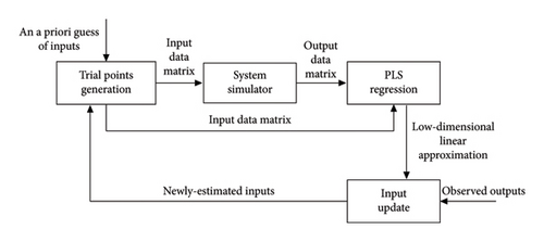
Figure 1 outlines the four main steps of the proposed calibration method: trial points generation, MATSim simulation, PLS regression and capacity update. The method is iterative, with each iteration comprising the four steps illustrated in the figure. Table 1 lists the most important symbols used in this paper and their meaning.

Table 1. Main symbols used in the proposed calibration method.

Symbol	Meaning
m	Dimension of input variables (capacities) and output variables (flows), i.e., number of links
m′	Number of links for which we have synthetic flow observations
m″	Number of links which have a non-zero true flow value
n	Number of trial points used in the PLS regression
δ	Variation coefficient in the step Generation and evaluation of trial points
pi	i-th loading vector in input space, size: m × 1
ti	i-th score vector in input space, size: n × 1
qi	i-th loading vector in output space, size: m × 1
ui	i-th score vector in output space, size: n × 1
a	The number of loading vector pairs used, i.e., dimension after dimensionality reduction operation
bi	The regression coefficient for i-th loading vector pair (of ui on ti) in PLS regression
s	Low dimensional representation of the estimated capacity vector, size: a × 1

4. Simulation Setup

The calibration method developed in Section 3 is evaluated in a MATSim simulation environment [36] for a toy network with two links and a large-scale urban network for Stockholm, Sweden. (Another 5-link toy model which illustrates loading vectors can be found in Wei [37]). For each network, demand and route choice are fixed. The route choice is generated from the simulation with the initial capacity guess. MATSim was chosen since we believe it provides a reasonable compromise between modelling complexity, flexibility, and computational efficiency for large networks.

Before starting a calibration method run, a synthetic true capacity vector is given. For the toy network, the synthetic true capacities are set manually to help us understand the mechanism of capacities in influencing network flows better. For the Stockholm network, a synthetic true capacity vector is generated by randomly varying each given link capacity in the range [0.85, 1.15] and then multiplying it by the initial guess of this link capacity in MATSim. For example, if a given link has an initial guess of capacity value of 1000, then its synthetic true capacity is generated between 850 and 1150, with a uniform distribution probability. It should be emphasized that the synthetic true capacity vector will not be used in the calibration method. It is only used in the evaluation of the performance of the method after calibration is done.

The MATSim network assignment package is used to assign the flows to routes and to compute network link flows. The simulation runs are made with a demand for the 6-7 a.m. period on a specific day.

For both networks, the method is run for 20 iterations (see Figure 1), this number is selected since the calibration result becomes stable after 20 iterations in most experiments, which can be regarded as a compromise between efficiency and accuracy. In step generation and evaluation of trial points, the initial variation parameter δ₀ = 0.1.

In addition, in step Joint linear approximation and dimensionality reduction, a sampling strategy is implemented intending for further improving the efficiency of the proposed calibration method: One does not only create a new set of trial points in every iteration, but also recycles all trial points from earlier iterations since introducing new trial points requires rerunning of the simulator to get the corresponding link flows, which significantly increases the overall computational time. In the first iteration, n = 101 trial points are generated in the simulator and used in the PLS regression. From the second iteration, 11 trial points are generated, and these newly generated trial points are added to the complete pool of trial points from all the previous iterations. Correspondingly, in the PLS regression from 2-nd iteration, the 101 trial points (out of 112) that are closest to the current capacity estimate are used. These values are picked after multiple trials, and it leads to satisfying efficiency and accuracy (which is shown in the result section). In terms of the initial experiments, the loading vector pair number a is set to 2 and 20 for the toy network and the Stockholm network, respectively. It is also assumed that the link flows are measured for all links, that is, m^′ = m, for the initial experiments.

4.1. Toy Network

The topology of the investigated toy network is shown in Figure 2. Each link has the same length of 1 km.

In this network, the true capacities of the two links are manually set to be $$ and the initial capacity guess is x⁽⁰⁾ = (800, 800). The purpose is to illustrate the results of the method for a small network with one bottleneck link (link 2) and a nonbottleneck link (link 1). The travel demand is 758 at 6 a.m., from the origin (O) to the destination (D) shown in Figure 2.

4.2. Stockholm Network

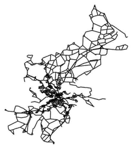
The Stockholm network has 22 547 links, with the topological network graph visualized in Figure 3.

In the Stockholm network, initial capacity values and travel demand are taken from a model developed by the Swedish Transport Administration. The route choice file is obtained by running the simulator with initial capacity values and the route choice remains unchanged during the calibration process. This range parameter is different and picked independently for each link.

5. Results

5.1. Results for Toy Network

For the toy network, we investigate flows and capacities on link 1 and link 2. Again, the synthetic true capacity values are $$, for which MATSim produces corresponding synthetic observed flow $$. The flow error function is here defined as

$$ ()

which has the same form as equation (20). Figure 4 shows the contour plot of f_toy values with respect to different x₁ and x₂ values. Further, the figure shows the iterative path of estimation of capacities $$ through 20 iterations.

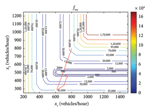
From the contour graph, we can see that we have a region of low f_toy values in a rectangular area 650 < x₁ < 1500, 470 < x₂ < 550. It indicates that in order to get a small f_toy value, x₂ is limited to a small range, while the range for x₁ is significantly larger, caused by link 2 being the bottleneck link. The iterative estimation of $$, starting from (800, 800), is illustrated as the red curve in the contour graph. The bottleneck link (link 2) achieves a better calibration result than the upstream link (link 1). The final estimated capacities are $$, which can be compared with the true capacities $$. The worse calibration result for $$ is caused by the objective function being flat in the x₁ dimension for x₂ values around the bottleneck capacity. This is an inherent characteristic of the network-wide capacity calibration problem.

It should be noted that the method is applied when the demand starts to be loaded into the network. Under this circumstance, the newly joined agents can travel through each link until the number of agents leaving the link reaches its capacity. In other words, the flow of each link is only determined by its own capacity, not the capacity of other links, and the travel demand on this link under this phase. These link flows provide information on where the bottlenecks are located. However, if the bottleneck is saturated, other links are experiencing either congestion or low flow due to bottlenecks. The flows of these links are bounded above by capacity of the bottleneck, and it is not possible to deduce which links are bottleneck links.

5.2. Results for Stockholm network

5.2.1. Experiment 1—Default Parameter Settings

Based on the method and experimental scenario introduced before, we construct Experiment 1 with the parameter settings given in Section 4 for the Stockholm network.

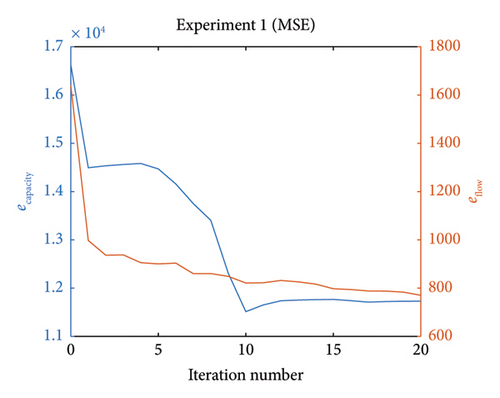
Figure 5 shows the MSE capacity error e_capacity and MSE flow error e_flow versus iteration numbers, where the error at iteration number 0 represents the error between initial guess and true values of capacities and flows, respectively. From Figure 5, both errors decrease as the iteration number increases. The fact that neither e_capacity nor e_flow goes to 0 is due to that for capacities, there exists many-to-one functional relationship when they are mapped onto flows, and for the flows, randomness exists in modeling of intersections.

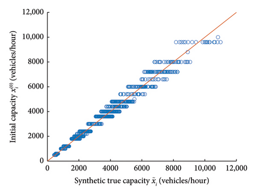
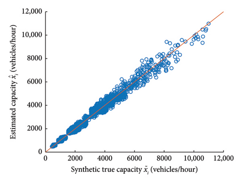
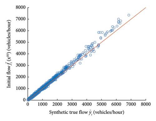
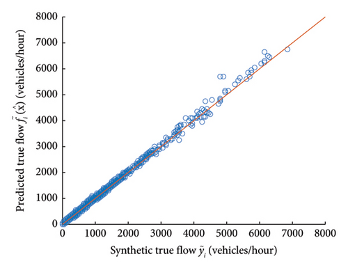
Figures 6 and 7 show the initial capacities and estimated capacities for all links in Experiment 1, respectively, and they are compared to the synthetic true capacities, (for initial values of capacities, there is a certain number of discrete values for all links, which comes from a very generalized classification of links from the data provider). It is visible that the estimated capacities are closer to the true ones when compared to the distance between initial capacities and true capacities. Similarly, Figures 8 and 9 show the initial flows and predicted flows for all links in Experiment 1, respectively, and they are compared to the observed flows. There is a clear improvement in reducing the difference between simulated flows and observed flows after calibration.

We also test the performance of an SPSA based calibration method [38] with 700 iterations, in which the step size parameters are selected through trial and error. The calibration result through iterations is shown in Figure 10.

Table 2 gives the initial error and the error after calibration for three error metrics presented in Section 4, where initial means the error before calibration, proposed represents our proposed method in this paper and SPSA represents the SPSA method. The results indicate that the proposed method performs better than the SPSA method in terms of calibration accuracy. The R² metric value does not change much after calibration since it is very close to 1 before capacities are calibrated. For the result from the SPSA method, even though the flow error decreases, we observe an increase in capacity error for metrics after calibration. Due to the many-to-one mapping from capacities to flows, it is possible that estimated capacities move further away from the true synthetic capacities when compared with initial capacities. It should be stressed that the proposed method requires about 8 h of running time on a PC with a RAM of 16 GB, while the time for running the counterpart SPSA method is roughly twice as long.

Table 2. Capacity error and flow error before and after calibration, for different methods and error metrics (Experiment 1).

		ecapacity	eflow
MSE	Initial	1.66 × 104	1640
	Proposed	1.17 × 104	770
	SPSA	1.93 × 104	1380
		$$	$$
R2	Initial	0.9822	0.9901
	Proposed	0.9875	0.9957
	SPSA	0.9793	0.9923
		$$	$$
MAPE	Initial	0.076	0.045
	Proposed	0.061	0.034
	SPSA	0.098	0.042

5.2.2. Experiment 2—Influence on Initial Variation Coefficient δ₀ in Trial Points Generation

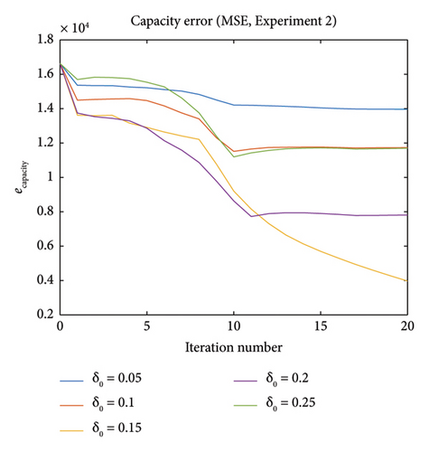
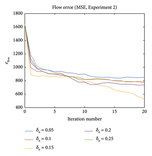
In Experiment 2, we investigate the influence of initial variation coefficient δ₀ in trial points generation (δ₀ = 0.05, 0.10, 0.15, 0.20, 0.25). Figures 11 and 12 show the capacity error e_capacity and flow error e_flow (both are in MSE metric) versus iteration numbers in Experiment 2. From the graphs, it can be observed that δ₀ = 0.15 case has the best calibration result. It indicates that the ideal δ₀ value should be neither too large (approximation will be inaccurate) nor too small (noise influence would be large).

5.2.3. Experiment 3—Influence on Initial Variation Coefficient δ₀ in Trial Points Generation

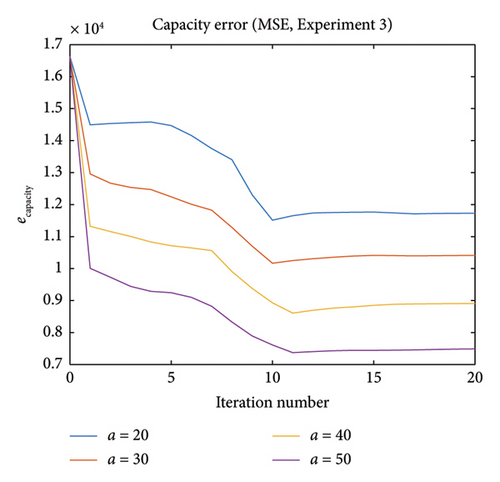
In Experiment 3, we investigate the influence of the number of loading vector pairs a in PLS regression (a = 20, 30, 40, 50). Figures 13 and 14 show the errors for different numbers of loading vector pairs used in PLS regression. More loading vector pairs being implemented indicate better results, but it should be noted that the introduction of more loading vectors leads to an increase in the running time. In this experiment, the running time for a = 50 is around 15 h.

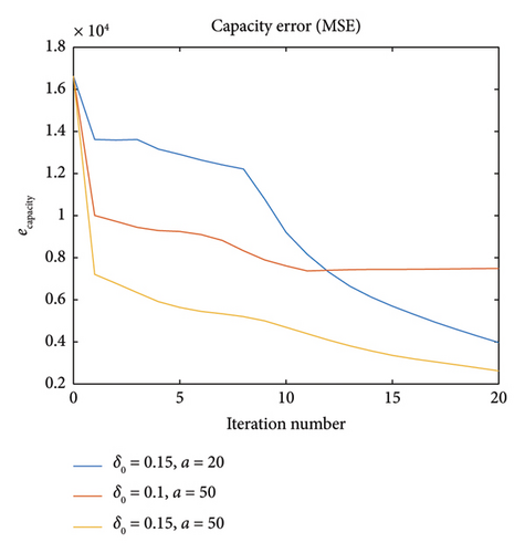
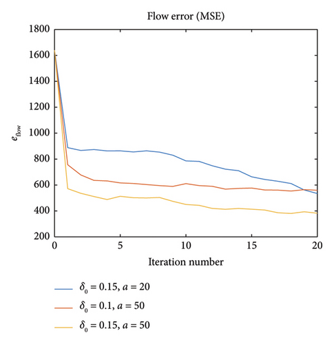
Experiments 2 and 3 suggest that with the proper combination of δ₀ and a, for example, δ₀ = 0.15 and a = 50, calibration can achieve even higher accuracy without significantly compromising computational efficiency. The result is shown in Figures 15 and 16, with the blue and red curves representing the best results for different δ₀ and a values in Experiment 2 and 3, respectively.

5.2.4. Experiment 4—Nonfully Known Flow Measurement Case

In real urban networks, it is not likely that sensor-based flow measurements are available on all links in the investigated network. In Experiment 4, the measured flows are known only for a fixed percentage of all links and these links are picked randomly. We investigate the effect of the proportion of link flow observations in the network (m^′/m = 100%, 75%, 50%, 25%, 1%). It should be stressed again that it only influences the objective function part in this method, and both MATSim and PLS regression still treat the output as m-dimensional. Figures 17 and 18 show the errors for different proportions.

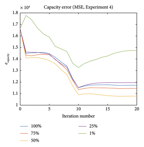
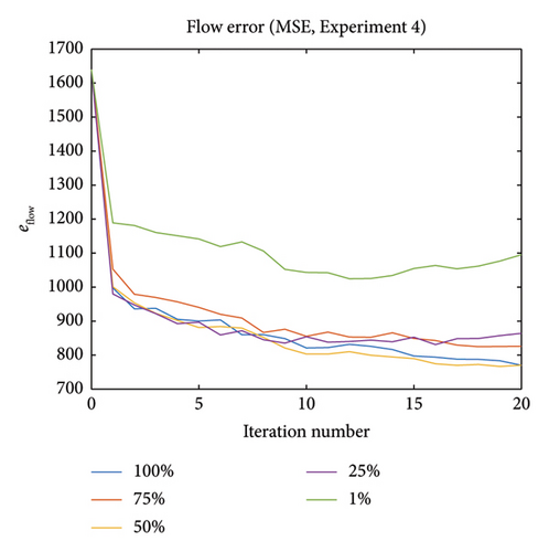
One can notice that the method performs well in terms of decreasing the flow error when m^′/m < 100%. For m^′/m = 25%, which means we only have link flow observations on 25% of the links, the performance is similar to the case of 100%. The 1% case performs worse compared to the 100% case regarding flow error, but the error still decreases compared to the initial one. In terms of capacity error, the final error is also smaller than the initial one for all percentage values in this Experiment 1. It is evident from this experiment that the method does not seem sensitive to m^′, unless the fraction is very small. One interesting aspect of this experiment is that the 50% case has better calibration result than 75% case, which is worth further investigation.

5.2.5. Experiment 5—Influence of Different Random Seeds in Generation of Trial Points

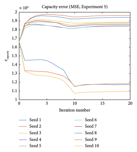
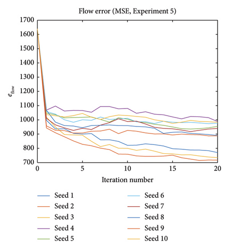
From Section 3, where we illustrate the whole proposed method, the generated trial points will influence the result of calibration. To test reliability of the proposed method, we can do multiple experiments to test the influence of random seeds in trial points generation. The generated trial points will influence the result of calibration. If different random seed settings are implemented, the calibration result will differ. In Experiment 5, we redo the work in Experiment 1, but with multiple different random seeds for generating trial points (10 seeds in total).

Figures 19 and 20 show both capacity and flow errors for different random seeds. The method performs well in terms of decreasing the flow error for all 10 seeds. However, for the capacity error, results for some seeds are even worse when compared to the initial error. It is because in the objective function, we don’t constrain the capacities to be close to their initial values. Moreover, it is known that the map between capacities and flows are many to one, the solver aims at finding capacity values which make the simulated flows similar to the observed ones without really taking care of the estimated capacities values. This phenomenon leads to Experiment 6.

5.2.6. Experiment 6—Influence of Adding Capacity Closeness Term in Optimization

In this experiment, we reformulate the expression of the optimization, including the terms making the capacity estimate be close to the initial guess. Note that, for simple reading, the formulation is given in a form without applying dimensionality reduction. In the experiment, it is transformed to a corresponding low-dimensional representation:

$$ ()

where $$ represents the initial values of capacities of all links. For the previous five experiments, it is equivalent to this formulation with weight w₂ = 0. Here, we test the calibration result for different w₂ values as well as for two different seeds (seed 1 and seed 5 from Experiment 5, which represent a ‘good’ and a ‘bad’ calibration results in terms of capacity error, respectively). The error graphs are shown in Figures 21, 22, 23, 24.

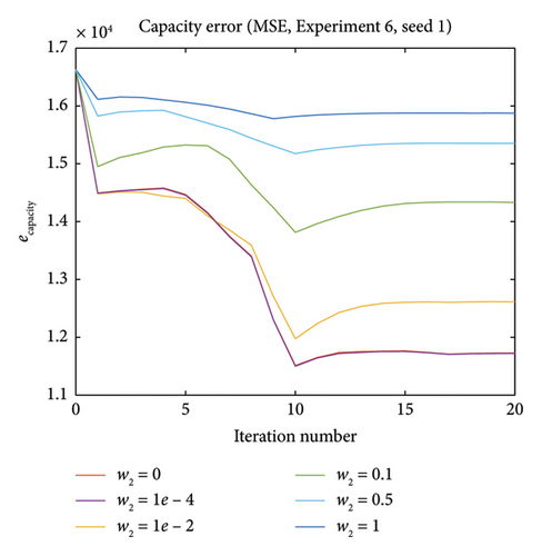
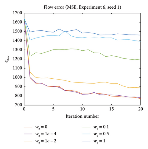
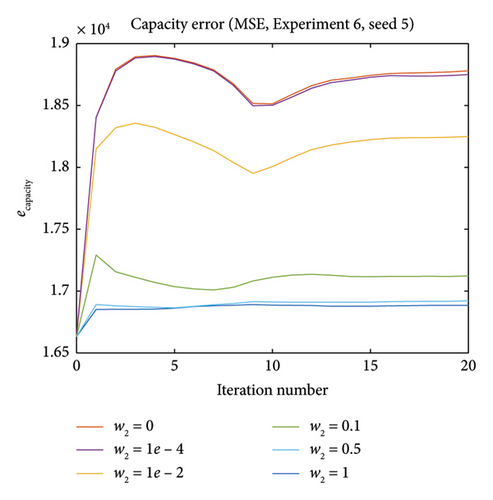
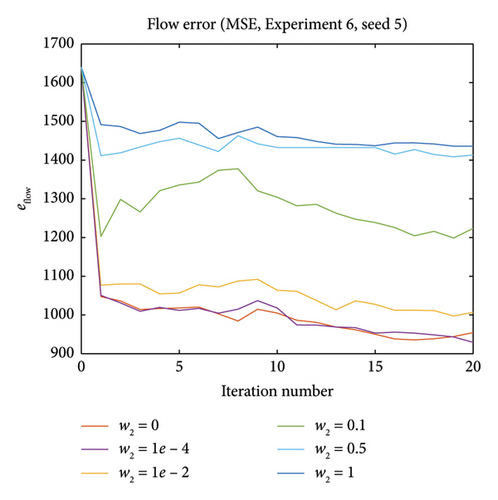
Intuitively, and as can be seen from the graphs, larger w₂ values give capacity estimations that is closer to the initial capacity, which on the other hand reduces the error reduction in flow. For seed 1, this means w₂ = 0 gives the best result for both errors since the existence of capacity error term in optimization will impede the calibration performance. For seed 5, higher w₂ values make the capacity error more stable, while on the other hand, the improvement on flow error is smaller.

6. Conclusion

Capacity calibration is a very challenging as well as an important problem in traffic modeling and network-wide approaches for capacity calibration are relatively unexplored in the literature. In this paper, we have highlighted the challenges in network-wide calibration.

Furthermore, we propose a novel method for network-wide capacity calibration of DTA models by implementing PLS regression to achieve dimensionality reduction. In our approach, the modified objective function can reduce the effect of these challenges and give a more stable result in the capacity dimension. We evaluate it by using simulation on a toy network as well as a large-scale urban network with promising results for the selected large-scale network in terms of both accuracy and efficiency when compared to the widely used SPSA method.

The assumption related to fixed and known OD demand is a major simplification of the problem and needs to be addressed in future work. However, new large-scale mobility data, like GPS probe data and mobile network data, with direct observations of route choice and OD demand, may support these assumptions in the future and can also be interesting to incorporate in the estimation method as future work.

Due to the theoretical foundation of the proposed method, one can expect it can be further implemented in OD calibration problems, which share a very similar structure. Future work includes analysis of the method across more networks, incorporating speed data for bottleneck detection, integrating network-wide and local approaches for capacity calibration, and utilizing different simulators as well as real-world data.

Disclosure

An earlier draft of this manuscript was presented in 10th Symposium of the European Association for Research in Transportation, hEART 2022, Leuven, Belgium, June 1–3, 2022, and was also presented as the main author’s Licentiate thesis in Linköping University, 2022. (Link: https://liu.diva-portal.org/smash/get/diva2:1689092/FULLTEXT02.pdf).

Conflicts of Interest

The authors declare no conflicts of interest.

Funding

This study was funded by the Trafikverket, 2018/134731 2021/22404.