Short-Term Passenger Flow Prediction Based on Federated Learning on the Urban Metro System
Abstract
Accurate short-term metro passenger flow prediction is critical for urban transit management, yet existing methods face two key challenges: (1) privacy risks from centralized data collection and (2) limited capability to model spatiotemporal dependencies. To address these issues, this study proposes a federated learning framework integrating convolutional neural networks (CNNs) and bidirectional gated recurrent units (BIGRU). Unlike conventional approaches that require raw data aggregation, our method facilitates collaborative model training across metro stations while keeping data stored locally. The CNN is employed to extract spatial patterns, such as passenger correlations between adjacent stations, while the BIGRU captures bidirectional temporal dynamics, including peak-hour evolution. This architecture effectively eliminates the need for sensitive data sharing. We validate the framework using real-world datasets from Shenzhen Metro, and our key innovations include a privacy-preserving mechanism through federated parameter aggregation, joint spatial-temporal feature learning without the need for raw data transmission, and enhanced generalization across heterogeneous stations.
1. Introduction
The imperative of precise short-term passenger flow prediction is underscored by its pivotal role in the formulation of traffic strategies and operational management within urban metro systems. This predictive modality is not simply a tool for decision-making within operational departments; it is also instrumental in managing emergent situations [1]. For instance, during peak traffic periods such as morning and evening rush hours, and in response to emergency scenarios, the ability to forecast passenger flow trajectories facilitates timely and effective reactions, thereby bolstering the system’s capacity to accommodate surges in ridership. The significance of high-accuracy, real-time short-term passenger flow forecasts in the orchestration and governance of urban metro networks cannot be overstated [2, 3].
- 1.
The challenge of inadequate sample sizes and feature sets in real-world metro passenger flow data has yet to be fully addressed. Most extant machine learning or deep learning methodologies for predicting metro passenger flow are predicated on the availability of ample historical data. However, these methods often do not account for scenarios where there may be a dearth of such historical data, which is a common occurrence in real-world prediction settings. The assumption that a predictor will have access to a large and comprehensive training dataset is not always tenable, leading to potential shortcomings in predictive performance when faced with limited training samples.
- 2.
The generalizability of predictive models remains a concern. Owing to the disparate scheduling and frequency of services across various metro operators and lines, the temporal and spatial dynamics of passenger flow data are inherently variable. Consequently, models trained on data from a single metro operator or line may not be directly transferrable to other contexts, necessitating enhancements to the model’s capacity to generalize across diverse operating environments.
- 3.
Data privacy considerations are of paramount importance. While data sharing among different metro operators could theoretically enrich the training dataset and thereby augment the model’s predictive prowess—especially with regard to weekend travel data where individual sample sizes are typically smaller—the high confidentiality demands associated with metro data inhibit such collaborative endeavors. Thus, developing solutions that address these privacy and confidentiality concerns is imperative.
Given these complexities, there is a compelling need to innovate and refine predictive models that can transcend the limitations of sample size, enhance generalizability, and comply with stringent privacy requirements. The pursuit of such advancements is essential in advancing the operational efficacy and service quality of urban metro systems.
This investigation addresses existing impediments in short-term metro passenger flow prediction through the implementation of a federated learning (FL)-based methodology. By integrating the collaborative training approach of FL, this study introduces an innovative prediction method that aligns with the distributed architecture of federated systems. Within this architecture, local clients—representing various metro companies—retain equal status, while the central server—potentially a trusted intermediary—facilitates the aggregation of intermediate results.
Significantly, this paper delineates a novel approach whereby the central server disseminates a global initial model to all clients. Utilizing their proprietary data, each client independently trains this model, thereby obviating the need to expose sensitive data externally. Upon completion of local training sessions, clients transmit model parameters, specifically the weights, to the central server. The server then performs an aggregation of these weights to refine the model, redistributing the updated version for subsequent rounds of client-side training. This FL paradigm not only preserves the privacy of client data but also leverages the collective data resources of all participating entities to enhance model accuracy and scenario generalization. FL offers significant advantages for subway passenger flow prediction. First, it effectively protects user privacy by ensuring that data remain local; only model updates are transmitted, thereby complying with data protection regulations. Second, FL facilitates collaboration among different subway systems, allowing them to jointly train models using their respective passenger flow data without sharing raw data. This approach enhances the model’s generalization capabilities, enabling it to better adapt to various cities and passenger flow patterns. In addition, this method supports real-time updates, allowing for quick adaptation to changes in passenger flow trends, such as during holidays or special events. Since only model updates are transmitted, communication costs are significantly reduced, making it particularly suitable for resource-constrained subway systems. Moreover, FL effectively addresses the issue of data imbalance by integrating data features from different regions, thereby minimizing the risk of overfitting in any specific area. Finally, the FL framework is highly flexible and scalable, making it easy to expand to include more participants, such as bus systems and taxi companies. This adaptability makes future traffic management and policy formulation more forward looking and comprehensive.
- 1.
Introduction of a FL collaborative training approach to model prediction. This method supplants the conventional centralized training modality with a distributed framework, decomposing complex problems into manageable subissues that are concurrently addressed by multiple devices. Such an approach maximizes computational resources across devices, significantly mitigating the computational burden on individual entities and enhancing overall efficiency. Furthermore, this strategy ensures the local retention of data, thereby safeguarding privacy.
- 2.
Development of the convolutional neural network–bidirectional gated recurrent unit (CNN–BIGRU) model. This model employs convolutional operations within CNNs to distill salient features from metro passenger flow data, followed by the application of BIGRU to discern long-term, bidirectional temporal dependencies within historical data, thereby capturing the dynamic fluctuations of station-level passenger flow.
- 3.
Empirical validation of the proposed model using passenger volume data from Shenzhen Metro system—specifically Lines 1, 2, and 3, each serving as a FL client. These clients operate in isolation, with no interclient data sharing. The initial CNN–BIGRU model is locally trained by each client through FL, followed by the server-led aggregation of the full weight parameters. The server then disseminates the averaged model parameters to the clients, thereby initiating subsequent rounds of communication and iteration.
The research thus contributes a scalable and privacy-preserving method for enhancing the accuracy and adaptability of short-term metro passenger flow predictions, offering a robust solution to the multifaceted challenges endemic to urban metro system operations.
The rest of this paper is organized as follows. In Section 2, a brief review of the current research on short-term metro passenger flow prediction and the development of FL is provided. In Section 3, we describe in detail the collaborative training method based on FL and the CNN–BIGRU model proposed in this paper. In Section 4, we have conducted an extensive comparison of short-term metro passenger flow prediction methods, and discussed the improvement of the FL collaborative training method proposed in this paper on ordinary machine learning models. Finally, in Section 5, we summarize the advantages and disadvantages of this study and point out potential directions for future work.
2. Related Work
This section provides a brief review of related research, including the development of metro passenger flow prediction and the recent progress in FL algorithms.
2.1. Metro Passenger Flow Prediction
Research on short-term passenger flow prediction can be divided into three main types: (1) statistical methods such as linear regression and Kalman filtering; (2) machine learning models such as neural networks; and (3) hybrid methods that combine optimization techniques with machine learning models. In the early stages, due to limited technology, most prediction methods relied on statistical models. For example, the authors in [6] used a time series model to process data from traffic detectors and predict passenger flow for the next 5 minutes. However, statistical methods have clear drawbacks. They perform poorly with nonlinear data, have complex designs, and work inefficiently, making them unsuitable for handling the complexity and volume of passenger flow data.
With the rapid growth of passenger flow data and its complex patterns, machine learning has gradually become the main method for short-term prediction. Compared with statistical models, machine learning methods can better handle nonlinear relationships and use multiple variables to improve prediction accuracy. For instance, studies such as [6, 7] and [8] used variables such as spatial-temporal data, historical passenger flow, and weather conditions to uncover hidden features in the data. In addition, parameter tuning has been introduced to improve accuracy. For example, the authors in [9] used an adaptive gray model that generated operators from historical passenger flow data to describe future trends while adjusting parameters automatically. Similarly, the authors in [7] applied fuzzy neural networks (FNNs) for urban road traffic flow prediction and combined it with an online training process to adjust model coefficients in real time, which improved its ability to adapt to traffic changes.
Although machine learning models outperform statistical methods, individual models also have limitations. For example, CNNs are good at extracting spatial features but struggle with temporal patterns, while LSTM models work well with time series data but lack spatial learning abilities. To solve this problem, researchers introduced hybrid models. For instance, the authors in [10] combined CNN and LSTM to extract both spatial and temporal features from railway passenger flow data, enabling predictions 20 min ahead. Similarly, the authors in [11] proposed a combined model using support vector regression (SVR) and LSTM, showing it performed better than single models in predicting unusual passenger flows. Besides combining models, researchers also used data processing and optimization techniques to improve prediction accuracy. For example, the authors in [12] presented a multisource signal fusion method that used a new signal decomposition algorithm along with traditional time series models. This method created a multiobjective framework to extract information from different data sources and predict upper and lower bounds for passenger flow.
In recent years, research on predicting passenger flow at the metro network level has increased. Unlike station-specific predictions, network-level predictions provide a broader view of how metro lines operate across a city. For example, the authors in [8] developed a spatiotemporal graph convolutional neural network (STGCNN). This model turned the metro network into a graph and used graph convolutional neural networks (GCNNs) to predict passenger flow (inflows and outflows) at all metro stations in the city. The authors in [13] proposed a deep learning-based model called EF-former, which focuses on the complex temporal evolution characteristics of urban rail transit (URT) passenger flow during large-scale events. This model extracts both global and local temporal dependencies through a parallel interactive attention module (PIAM) and multiscale causal multihead self-attention (MSC-MSA), combining regular outflow and additional outflow data to predict the occurrence time of surges in passenger flow. Experimental results demonstrate that EF-former significantly outperforms traditional benchmark models in terms of prediction accuracy on large-scale event datasets, and ablation experiments validate the effectiveness of its key modules. Similarly, the authors in [14] designed the PAG-STAN framework to address the challenges of real-time, sparse, and high-dimensional origin-destination (OD) demand forecasting during the pandemic. This framework generates a dense demand matrix through a Real-Time OD Estimation Module and a Dynamic Compression Module, integrating heterogeneous data with a Masked Physical Guidance Loss Function (MPG-loss) to enhance model interpretability. Experiments show that PAG-STAN exhibits robustness in both pandemic and regular scenarios, with ablation studies further confirming the necessity of its module design. Meanwhile, the authors in [15] introduced a traffic state estimation method that combines computational graphs with Physics-Informed Deep Learning (PIDL). This method determines the fundamental parameters of traffic using computational graphs and embeds them into the PIDL framework, leveraging the dual advantages of data-driven and model-driven approaches to reconstruct segment traffic states in sparse data scenarios, such as loop detectors and probe vehicles. Experimental results indicate that PIDL outperforms pure deep learning and other baseline models, validating the feasibility of integrating domain knowledge with deep learning in traffic control.
2.2. FL Algorithms
FL is a concept introduced in recent years and is widely used in fields such as healthcare and banking. Its goal is to build a unified model using distributed datasets while keeping the data private. The framework usually includes two stages: model training and model inference. During training, participants (clients) share encrypted information related to the model instead of raw data, which protects their data privacy.
Research on FL focuses on two main areas: algorithms and communication. In terms of algorithms, researchers work on reducing the cost of model updates and data transmission, improving communication efficiency. For example, some studies suggest uploading only significant updates, compressing gradients, or using sparse updates with momentum to save bandwidth and speed up training. For communication, when training time is limited, solutions include adjusting local computation steps to reduce global gradient differences or selecting the maximum number of devices to participate. Structural updates and heuristic updates are common ways to lower the communication cost between clients. The Federated Averaging (FedAvg) algorithm is widely used because it requires fewer communication cycles [16–19].
For example, the authors in [20] improved FL by addressing communication costs, retention issues, and fault tolerance. The study showed that multitask learning could solve statistical problems by creating task similarity graphs, which act as communication graphs. During updates, clients collaborate with others that share similar tasks, reducing unnecessary communication with unrelated clients. Another study [21] proposed a FL approach where client data reflects different tasks, and the global model adapts to these tasks. Using Model-Agnostic Metalearning (MAML), the global model can be fine-tuned for individual clients, helping it adapt to new tasks. Recently, researchers have also focused on improving FL efficiency by enhancing device performance or reducing communication delays. For example, the authors in [22] explored ways to lower communication delays to make FL frameworks faster and more cost-effective, and they validated this idea through simulations.
In addition, many privacy-preserving techniques have been proposed. For example, the authors in [23] combined blockchain with FL to protect privacy through hierarchical aggregation and ensure data traceability. Moreover, the authors in [24] introduced a federated metalearning system called Padp-Federmeta to address the impact of nonindependent and identically distributed (non-IID) data on prediction accuracy. This system allowed personalized privacy handling for clients and smoothed gradient fluctuations during communication, which sped up convergence. The authors in [25] proposed a hybrid short-term subway passenger flow prediction model called DEASeq2Seq, which significantly improves prediction accuracy through three phases: decomposition, integration, and prediction, utilizing a fully empirical mode decomposition technique that adapts to noise. Similarly, the authors in [26] employed a CNN–LSTM model to analyze the impact of spatial features such as relative location, specific location, and land use on passenger flow prediction. The study found that relative location and the distance of stations from the city center significantly affect prediction accuracy. Meanwhile, the authors in [27] introduced the ASC–GRU model, which combines multigraph convolutional networks with gated recurrent units. This model not only takes into account the topological relationships of the subway network but also incorporates non-Euclidean spatial dependencies such as adjacency, similarity, and correlation. Testing results show that this model outperforms other benchmark models in predicting passenger flow over long-time intervals and across large-scale networks.
3. Methodology
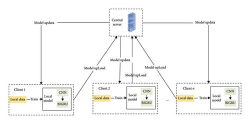
The FL framework proposed in this paper is composed of local models at the client side working in collaboration with a central server, as illustrated in Figure 1. On the client side, the CNN–BIGRU prediction model is independently trained based on local historical passenger flow data. The CNN module extracts local spatial features of the passenger flow sequence (such as mutation patterns in adjacent time periods) through multiscale convolutional kernels. Subsequently, the BIGRU module employs a bidirectional gating mechanism—where the forward GRU captures historical trends, and the backward GRU learns potential future dependencies—to model the short-term and long-term temporal dynamics, ultimately outputting the passenger flow predictions for the next N steps. At the FL level, after the local training is completed at each client, the model parameters are uploaded to the central server via a secure channel. The server utilizes the FedAvg algorithm to perform weighted aggregation of the global parameters (with weights determined by the proportion of data from each client), generating a unified optimized global model that is distributed to all clients to initiate the next round of training. This process achieves a closed-loop iteration through “local training ⟶ parameter encryption and upload ⟶ global aggregation ⟶ model distribution,” balancing privacy protection (with the original data always retained locally) and knowledge sharing (through the integration of cross-site temporal and spatial patterns).
3.1. CNN–BIGRU Model
Both CNN and GRU can be used to capture effective features in network data. CNN extracts the features of network data layer by layer through convolution calculation, and GRU improves the accuracy of the model by capturing the dependence of long-term information in ordered data. Although CNN and GRU can effectively extract hidden features, they cannot completely capture the data sequence information from back to front, so it is impossible to better extract hidden features in the original data. To solve this problem, this paper uses a hybrid neural network that combines CNN and BIGRU to capture hidden data temporal sequence features.
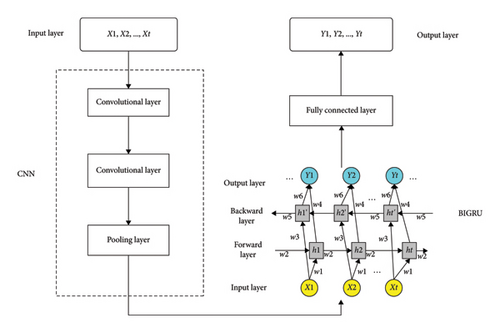
Overly complex network structure often affects the convergence efficiency of FL, so a simple CNN with 2 convolutional layers and 1 fully connected layer is used to train the model. The specific structure is shown in Figure 2.
We have added a standardized list of abbreviations in the appendix, organized alphabetically for easy reference (Table A3).
3.1.1. CNNs
CNN has the characteristics of local connection and weight sharing, which can efficiently extract input features. The process of CNN calculation is that nonlinear activation function is introduced after convolution. The pooling layer is used for feature selection to reduce the number of parameters. After the feature is extracted by convolutional neural network, it is generally sent to the full connection layer [28].
3.1.2. BIGRU
The GRU model is a variant of the LSTM model, which combines the forget gate and the input gate in the LSTM model into a single update gate. It also mixes cell state and hidden state, as well as some other changes. This allows it to achieve efficiencies similar to LSTM in a simpler structure [29].
In 1997, Schuster and Paliwal proposed a bidirectional recurrent neural network (BiRNN) and used BiRNN to conduct speech recognition experiments [30, 31]. One-way RNN can only extract from previous inputs to predict the current state, but BiRNN extract future data to improve their accuracy. When predicting, BiRNN takes both forward and backward values as input. BiRNNs also apply to BiLSTM and BIGRU. In passenger flow prediction, the output at this time is closely related to the information of the previous moment and the information of the next moment. Therefore, this paper selects the BIGRU model to learn the dynamic change law of passenger flow at metro stations [32].
3.2. FL Collaborative Training
Artificial intelligence models require large datasets for training to achieve optimal performance. However, data privacy concerns have become a major barrier, as organizations and individuals are often unwilling to share their data [33, 34]. To address this issue, FL has emerged as an effective solution. FL enables collaborative model training by aggregating local model updates from multiple parties without sharing raw data. Participants in FL can be enterprises, individuals, or devices, each with independent datasets and training processes. By ensuring that data remain local, FL protects privacy while facilitating the construction of a global machine learning model. Unlike traditional distributed machine learning, FL achieves joint model building without moving data out of local storage.
- 1.
Collaboration: FL involves two or more participants jointly training a shared machine learning model using their local datasets.
- 2.
Data privacy: data remain with the owner and does not leave the participant during the training process.
- 3.
Secure communication: communication between participants can be encrypted, ensuring that no party can infer others’ data from shared information.
- 4.
Model performance: the collaboratively trained model should perform comparably to models trained using traditional methods.
FL typically involves two roles: local clients and a central server. Local clients provide data and perform local training, while the server aggregates the updates to build the global model. For tasks such as short-term metro passenger flow prediction, FL enables clients to protect data privacy while collaboratively training models, improving accuracy and generalization across scenarios.
The architecture of FL is illustrated in Figure 3.
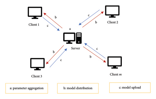
The FL collaborative training process is as follows, which mainly includes two parts [21].
3.2.1. Model Distribution
The model is pretrained on the server side to obtain the server-side model weight parameter W. Through the communication network, W is distributed to the local end of each federation participating in the training Gi. Each Gi receives the W distributed by the server, updates the local model weight parameter Wi, and then uses its own dataset Ddata as the local training sample set to conduct local training and update Wi.
3.2.2. Model Upload
After the local model is trained, each local Gi uploads the model weight parameters to the server through the communication network, but there are multiple transmission methods during the parameter transmission process.
In order to avoid the risk of reverse pushing out the corresponding data samples due to the leakage of gradient parameters, this paper adopts the method of directly transmitting the complete weight parameters without transmitting the gradient and uploads the overall model weight parameter Gi instead of the gradient generated during the training of a single data sample after the local model training of the participants is completed.
The algorithm is as follows (see Algorithm 1):
-
Algorithm 1: FL collaborative training.
-
Input:
-
Global model weight W (pretrained on the server)
-
Participating clients G = {G1, G2, … , Gn}
-
Local datasets Ddata for each client Gi
-
Number of training rounds R
-
Learning rate η
-
Output:
-
Updated global model weights W
-
Process:
- 1.
Initialization:
-
Server initializes global model weight W.
- 2.
Model Distribution:
-
For each training round r = 1 to R do:
-
a. Server distributes the global model weight W to all clients Gi ∈ G.
- 3.
Local Training (on each client Gi):
-
For each client Gi in parallel do:
-
a. Receive W from the server.
-
b. Use local dataset Ddata to update local model weights Wi:
-
Wi ⟵ Wi − η ∗ ∇L (Wi; Ddata)
-
//Perform optimization using local dataset
-
c. Complete local training and obtain updated local weights Wi.
- 4.
Model Upload:
-
Each client Gi uploads its updated local weights Wi to the server.
- 5.
Aggregate Weights (on the server):
-
a. Server aggregates the weights uploaded by all clients:
-
W ⟵ ∑(ni ∗ Wi)/∑ni
-
//Weighted averaging where ni is the size of client Gi’s dataset
- 6.
Repeat Until Convergence:
-
Repeat Steps 2–5 until the global model converges or the maximum number of rounds R is reached.
- 7.
Output the Final Model:
-
Return the final global model weights W.
The advantages of FL are obvious: compared with traditional centralized model training methods, FL does not need to transmit a large amount of data to a single device through the network, which saves a lot of network communication consumption. At the same time, because there is no need to centralize a large amount of data on one device for calculation, it also saves the computing power of each device. The collaborative training principle of FL is equivalent to decomposing a very complex overall problem into multiple relatively simple small problems and then using multiple devices to calculate these small problems. This training mode makes full use of the computing power of each device, and the computing pressure spread out by each device is much smaller than that of centralized computing. This greatly improves computing efficiency, and because only the weight parameters of the model are transmitted through the network, the data of each client can be retained locally, which greatly avoids the issue of data privacy disclosure. It can be said that the emergence of FL has transformed users from bystanders of artificial intelligence to participants in the development of artificial intelligence.
3.3. Model Complexity Analysis
3.3.1. The Computational Complexity of CNN–BIGRU
Among them, H′∗W′: output feature map size. C2: number of channels. K2: convolutional kernel size. The number of convolutional layers is 2.
Among them, T: enter the sequence length. din: GRU input dimension. dhidden: the number of GRU hidden units. LBiGRU: BiGRU layers (set to 1).
Among them, dinput: fully connected layer input dimension. doutput: the fully connected layer outputs dimensions.
3.3.2. Overall Complexity of FL Framework
Among them, N: the number of participating clients. |θ|: the total number of model parameters.
Among them, E: number of iterations for local training. n: the sample size of local data for each client. Omodel: the single computation complexity of the model (forward and backward).
4. Experimental Analysis
4.1. Data Description
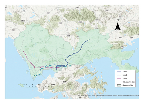
This paper selects the passenger flow data of Shenzhen Metro in Guangdong Province, China. The main source of data is metro IC cards. The passenger flow at each metro station is calculated based on the metro gate swiping records. Shenzhen Metro has a total of 11 lines and 166 metro stations. This paper selects the monthly metro passenger flow data from May 1 to May 31, 2019. According to the actual operation time of the metro system, this paper only uses the records from 6 a.m. to 11 p.m. We summarize the collected data. Specifically, we summarize the passenger flow data at each station at 10 minutes intervals and distinguish between inbound and outbound passenger flows. In this paper, the most representative Lines 1, 2, and 3 are selected as the research object. The specific metro route map is shown in Figure 4.
4.2. Comparative Experiments
Taking the three Lines 1, 2, and 3 in Shenzhen Metro system as three local clients, the inbound passenger flow data of the transfer station on each line were selected for experimentation. In this paper, the number of communication rounds for FL is set to 50. CPU: AMD Ryzen 7 5800H (8 cores, 16 threads, with a base frequency of 3.2 GHz); GPU: NVIDIA GeForce RTX 3070 (8 GB VRAM, with 5888 CUDA cores); and RAM: 16 GB DDR4. Both the server and client are logically separated through process isolation, simulating a distributed training scenario with a total of three simulated clients, each allocated an independent memory partition. The analysis results of model performance and hardware adaptability are provided in Appendix Table A2.
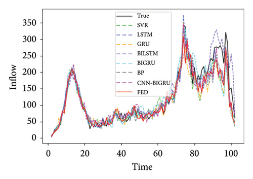
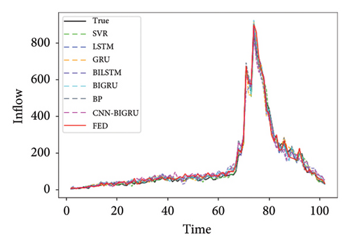
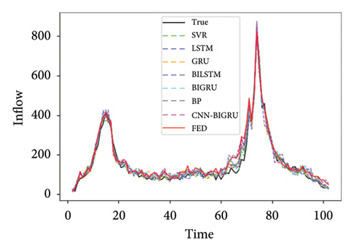
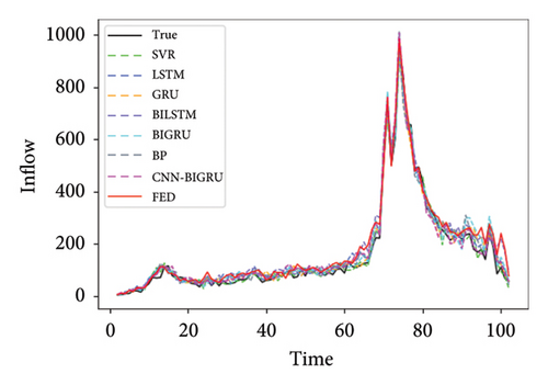
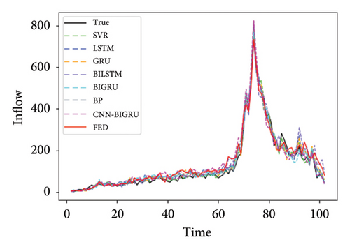
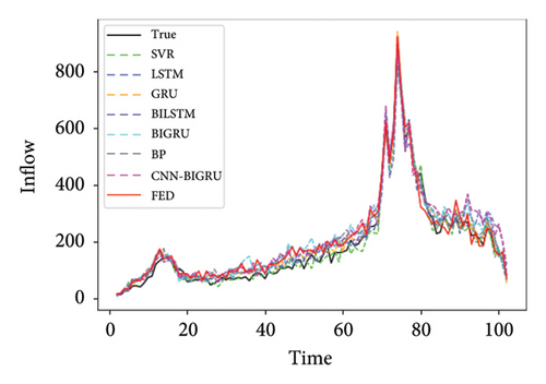
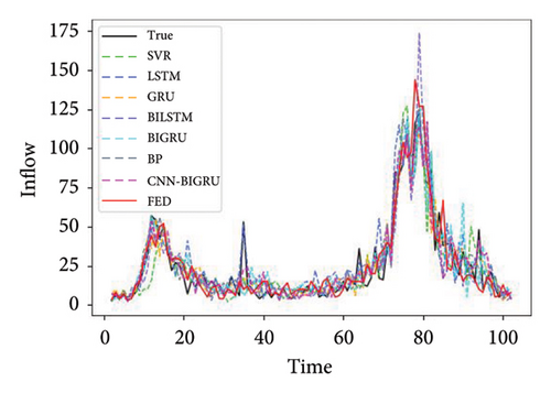
SVR, LSTM, GRU, BILSTM, BIGRU, and BP were selected as the local comparison model. Abbreviations of station names in Figure 5 and Table 1 are as follows. The efficiency of model training is shown in Appendix Table 2.
| BAZX | CGM | GS | GWGY | |||||
|---|---|---|---|---|---|---|---|---|
| RMSE | MAE | RMSE | MAE | RMSE | MAE | RMSE | MAE | |
| SVR | 34.23 | 27.47 | 22.47 | 18.18 | 23.79 | 19.13 | 40.06 | 31.35 |
| LSTM | 25.28 | 19.08 | 14.3 | 10.37 | 16.18 | 13.46 | 25.5 | 18.95 |
| GRU | 26.76 | 21.46 | 14.35 | 10.92 | 16.16 | 13.22 | 25.05 | 18.46 |
| BILSTM | 21.79 | 16.32 | 10.19 | 8.61 | 11.95 | 9.01 | 20.65 | 15.14 |
| BIGRU | 23.68 | 17.85 | 10.42 | 8.93 | 10.85 | 8.96 | 21.96 | 16.31 |
| BP | 33.61 | 26.7 | 23.5 | 18.47 | 25.89 | 21.19 | 43.62 | 32.1 |
| CNN–BIGRU | 18.89 | 13.03 | 7.16 | 4.35 | 9.2 | 6.23 | 18.31 | 11.75 |
| FED | 18.66 | 13.59 | 7.3 | 4.72 | 9.47 | 6.31 | 19.29 | 12.7 |
| HZZX | LJ | QHW | ATS | |||||
| RMSE | MAE | RMSE | MAE | RMSE | MAE | RMSE | MAE | |
| SVR | 23.02 | 18.33 | 35.52 | 20.43 | 16.89 | 13.39 | 12.04 | 9.32 |
| LSTM | 17.06 | 12.49 | 29.86 | 18.25 | 12.9 | 10.39 | 8.05 | 6.33 |
| GRU | 17.21 | 12.84 | 27.37 | 16.08 | 11.88 | 9.38 | 8.02 | 6.32 |
| BILSTM | 16.8 | 12.25 | 25.07 | 15.1 | 10.86 | 8.32 | 7.03 | 5.29 |
| BIGRU | 17.71 | 13.05 | 23.93 | 14.51 | 9.9 | 7.41 | 7.06 | 5.36 |
| BP | 25.22 | 20.8 | 38.77 | 26.2 | 18.94 | 16.45 | 14.06 | 11.32 |
| CNN–BIGRU | 14.76 | 10.16 | 20.41 | 12.79 | 8.86 | 6.31 | 4.04 | 3.38 |
| FED | 15.07 | 10.84 | 22.4 | 13.6 | 6.96 | 5.52 | 4.08 | 3.33 |
| DJY | FT | GSB | HH | |||||
| RMSE | MAE | RMSE | MAE | RMSE | MAE | RMSE | MAE | |
| SVR | 34.29 | 28.55 | 39.77 | 31.77 | 25.78 | 20.84 | 32.02 | 26.44 |
| LSTM | 27.16 | 21.42 | 29.46 | 18.6 | 17.67 | 13.01 | 25.85 | 20.1 |
| GRU | 25.46 | 20.29 | 28.62 | 20.85 | 15.73 | 11.11 | 24.59 | 19.4 |
| BILSTM | 23.75 | 19.05 | 27.51 | 20.94 | 15.05 | 11.16 | 23.31 | 17.65 |
| BIGRU | 22.9 | 18.42 | 26.76 | 17.84 | 13.73 | 9.85 | 22.55 | 17.36 |
| BP | 36.19 | 30.53 | 41.78 | 31.84 | 27.7 | 21.95 | 35.47 | 29.91 |
| CNN–BIGRU | 19.46 | 15.96 | 23.77 | 17.43 | 7.75 | 6.17 | 19.23 | 14.17 |
| FED | 20.58 | 16.53 | 25.45 | 17.56 | 7.79 | 5.96 | 16.47 | 11.22 |
| HQB | HBL | JT | SJZC | |||||
| RMSE | MAE | RMSE | MAE | RMSE | MAE | RMSE | MAE | |
| SVR | 30.47 | 25.52 | 32.53 | 27.41 | 28.77 | 23.08 | 37.44 | 29.41 |
| LSTM | 20.02 | 16.06 | 23.45 | 17.96 | 19.69 | 15.09 | 24.38 | 20.04 |
| GRU | 18.99 | 14.76 | 22.79 | 17.64 | 18.67 | 14.67 | 23.33 | 19.34 |
| BILSTM | 17.33 | 13.47 | 21.8 | 16.45 | 15.96 | 12.11 | 19.89 | 16.02 |
| BIGRU | 16.15 | 12.3 | 20.18 | 15.76 | 15.77 | 12.99 | 19.12 | 15.87 |
| BP | 32.26 | 27.66 | 34.5 | 28.46 | 30.66 | 24.95 | 38.94 | 30.61 |
| CNN–BIGRU | 16.01 | 12.19 | 17.88 | 13.72 | 15.91 | 12.07 | 17.6 | 14.41 |
| FED | 15.14 | 11.5 | 16.36 | 13.26 | 15.79 | 13.13 | 16.79 | 13.93 |
| SMZX | HL | HX | LHC | |||||
| RMSE | MAE | RMSE | MAE | RMSE | MAE | RMSE | MAE | |
| SVR | 34.38 | 26.45 | 25.32 | 21.08 | 30.1 | 24.6 | 22.31 | 18.73 |
| LSTM | 26.17 | 20.84 | 17.04 | 13.61 | 19 | 14.46 | 15.26 | 13.64 |
| GRU | 24.71 | 19.14 | 15.42 | 12.97 | 18.93 | 14.96 | 15.33 | 13.78 |
| BILSTM | 22.43 | 18.33 | 14.23 | 11.92 | 17.78 | 14.4 | 12.25 | 9.68 |
| BIGRU | 22.46 | 18.42 | 13.76 | 11.03 | 16.56 | 13.21 | 12.36 | 9.77 |
| BP | 44.25 | 35.86 | 27.4 | 22.67 | 31.96 | 25.82 | 25.4 | 20.76 |
| CNN–BIGRU | 20.17 | 17.13 | 10.23 | 7.99 | 15.41 | 12.58 | 10.23 | 7.65 |
| FED | 19.39 | 16.88 | 9.4 | 6.76 | 13.67 | 11.96 | 10.52 | 7.84 |
| SNG | SS | TB | TXL | |||||
| RMSE | MAE | RMSE | MAE | RMSE | MAE | RMSE | MAE | |
| SVR | 40.03 | 29.57 | 26.76 | 21.55 | 24.22 | 20.32 | 29.49 | 22.69 |
| LSTM | 29.01 | 21.52 | 20.97 | 16.8 | 18.04 | 14.25 | 22.79 | 17.36 |
| GRU | 25.16 | 18.12 | 18.97 | 15.76 | 18.03 | 14.02 | 21.27 | 16.49 |
| BILSTM | 23.56 | 17.08 | 16.7 | 13.48 | 15.04 | 12.11 | 20.15 | 14.29 |
| BIGRU | 21.78 | 15.73 | 16.84 | 13.66 | 13.45 | 10.77 | 19.59 | 12.68 |
| BP | 39.75 | 30.95 | 27.3 | 22.07 | 27.01 | 22.05 | 30.27 | 22.51 |
| CNN–BIGRU | 19.4 | 14.7 | 14.77 | 11.46 | 13.16 | 10.2 | 16.38 | 13.62 |
| FED | 18.88 | 14.37 | 14.92 | 11.08 | 13.35 | 10.26 | 14.02 | 12.61 |
- Note: The bold font represents the smallest value (best).
| CNN–BIGRU | FED | |||
|---|---|---|---|---|
| RMSE | MAE | RMSE | MAE | |
| CGM | 34.12 | 28.72 | 14.26 | 11.51 |
| HZZX | 32.01 | 27.11 | 18.52 | 14.83 |
| ATS | 26.87 | 23.61 | 13.03 | 11.29 |
| DJY | 29.17 | 22.01 | 19.72 | 13.95 |
| SNG | 28.18 | 22.65 | 12.19 | 10.66 |
| TB | 31.41 | 25.06 | 15.38 | 12.63 |
Table 1 shows the prediction performance of short-term passenger flow prediction model FED based on FL, local model CNN–BIGRU, and other machine learning models on the three lines of Shenzhen Metro. It can be seen from Figure 4 that the accuracy of the CNN–BIGRU model proposed in this paper is higher than that of other machine learning models among the local learning training models. Among these local comparison models, the prediction performance of SVR and BP models is the worst, which caused by the fact that these two models simply input the historical passenger flow data of the station and cannot extract the space–time information contained in the historical passenger flow data. Compared with these two models, the LSTM and GRU models perform better. This is because the LSTM and GRU models can effectively extract the time series information in the historical passenger flow data of each station and the long-term dependency relationship among them. This also shows the importance of time information in metro passenger flow prediction. Compared with the ordinary LSTM and GRU models, the BILSTM and BIGRU models have more complete network structures and more sufficient forward and backward information extraction from the historical passenger flow data of each station, which also makes them perform better in prediction than the ordinary LSTM and GRU models. In the CNN–BIGRU model, CNN extracts the characteristics of passenger flow data layer by layer through convolution calculation. BIGRU further improves the prediction performance of the model by capturing the dependency of medium and long-term information of ordered data. The final prediction performance is also due to a single BILSTM and BIGRU model. This also proves that the CNN–BIGRU model selected in this paper as the local prediction model is effective and accurate.
It can also be seen from Table 1 that in most cases, the RMSE value of FED model and CNN–BIGRU model is close to the MAE value. In most sites, the prediction performance of the model using FL training is basically the same as that of the model using ordinary deep learning training. This shows that the prediction accuracy of FL can reach or even exceed the average level of ordinary deep learning models. It also proves that the collaborative training mode of FL is feasible for metro passenger flow prediction.
In order to comprehensively demonstrate the effectiveness of the method proposed in this paper and enhance the credibility of the experimental results. We used statistical testing methods to verify the significance of performance differences. Figure 6 shows the prediction error distribution of the subway passenger flow prediction method based on FL proposed in this paper.
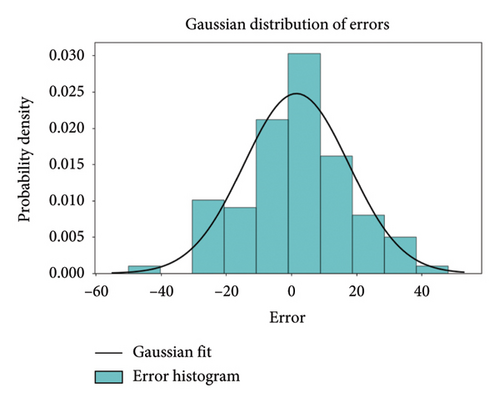
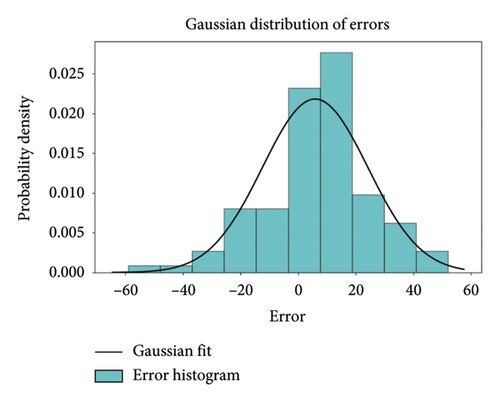
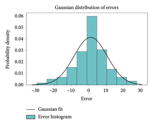
Figure 6 shows the distribution of prediction errors based on three clients (LINE1, LINE2, and LINE3), systematically validating the effectiveness and robustness of the FL framework in subway passenger flow prediction from a statistical perspective. Through Gaussian fitting analysis, the errors for the LINE1 client are primarily concentrated in the range of −20–+20 (with a peak density of 0.025), having a mean of −1.2 and a standard deviation of σ ≈ 12.3, exhibiting a symmetrical distribution without significant systematic bias. The error range for the LINE2 client is broader (−60 to +60), with the main density concentrated between −30 and + 30, a mean of +4.8, and a standard deviation of σ ≈ 25.6. This indicates a slight right skew (with a higher proportion of positive errors), suggesting that the characteristics of its data are related to frequent fluctuations in passenger flow during holidays, resulting in the model’s insufficient prediction of positive deviations. In contrast, the error distribution for the LINE3 client is the most concentrated, ranging from −30 to +30, with a peak density reaching 0.06. The mean is −0.5 and the standard deviation is σ ≈ 8.7, reflecting the stability of commuter-dominated passenger flow on this line.
The CNN–BIGRU model achieves precise modeling of the spatiotemporal characteristics of subway passenger flow through a deep integration of CNNs and BIGRU. CNN excels at extracting local spatial dependencies—such as the correlations in passenger flow between adjacent stations—and multiscale spatial patterns, like regional passenger flow diffusion. Meanwhile, BIGRU captures long-term temporal dependencies through its bidirectional gating mechanism, which reflects the dynamic evolution during peak hours, resulting in a joint representation of “spatial and temporal” features. The FL framework further enhances the applicability of this architecture. Its distributed training mechanism allows each station to locally train its CNN–BIGRU model while only sharing encrypted model parameters instead of raw data. This approach not only protects user privacy and sensitive information (in compliance with regulations such as GDPR) but also addresses the issue of data silos. In addition, the federated aggregation algorithm merges the local model parameters from various stations, implicitly learning global spatiotemporal patterns—such as holiday passenger flow trends across the entire network—while preserving the unique features of local models, such as specific stations’ unusual passenger flow patterns. This process enhances the model’s generalization ability and robustness when dealing with complex and heterogeneous (non-IID) data scenarios.
The framework demonstrates significant advantages in practical applications. First, the parameter compression and asynchronous update strategies inherent in FL greatly reduce the communication overhead between stations, accommodating the bandwidth limitations of distributed subway systems. Furthermore, the localized training and incremental update mechanisms support real-time responses to sudden events (such as temporary flow restrictions), avoiding the delays associated with full retraining in traditional centralized models. Second, this framework offers both scalability and security: new stations can swiftly join the federated network and utilize the global model to initialize local prediction tasks, while ensuring that data remain local to reduce the risk of centralized data breaches. Lastly, through cross-regional federated collaboration (for instance, in multicity subway networks), the model can leverage the global data sparsity to enhance prediction accuracy (such as transferring learning from niche station patterns) while avoiding the direct sharing of sensitive data. This “global-local” collaborative optimization mechanism provides high-accuracy, privacy-preserving, and low-latency predictive support for dynamic scheduling in smart transportation—such as emergency resource allocation and train frequency adjustments—facilitating the evolution of subway systems toward greater intelligence and resilience.
4.3. Model Stability Experiment
To verify the stability of the subway flow prediction method based on FL proposed in this article, we designed a series of control experiments. In the experiment, the data loss rates of all clients were randomly set to 5%, 10%, 30%, and 50%, respectively. Through this approach, we investigated the predictive performance of CNN–BIGRU and FED models under abnormal data conditions, as shown in Figure 7.
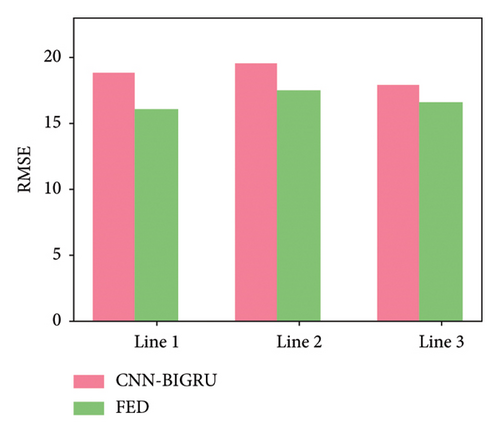

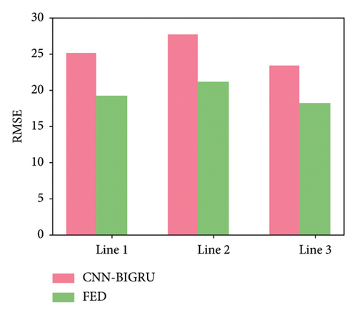
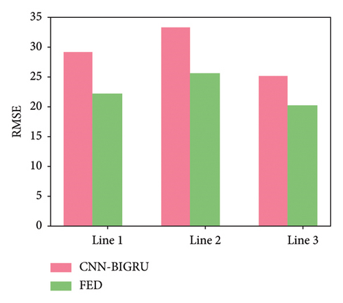
According to the experimental results shown in Figure 7, it can be seen that as the data missing rate increases, the performance of the two models gradually differs. For the 5% and 10% missing rates, the performance of the two models is relatively similar and the RMSE value is low. Both can effectively predict subway traffic in the case of minimal data loss. However, as the missing rate reached 30% and 50%, the RMSE of the CNN–BIGRU model significantly increased, and the prediction error gradually increased, showing poor qualitative performance. Relatively speaking, the predictive performance of the FED model is relatively stable, and even in cases of high data loss, the RMSE value is still lower than that of the CNN–BIGRU model. This indicates that FL methods have strong robustness and can effectively handle the impact of data loss in multiclient collaboration.
From these results, it can be seen that the FED model based on FL exhibits significant advantages when facing data loss. Especially in cases of severe data loss, FED models can rely on data from other clients for compensation, thereby reducing the impact of single client data loss on prediction results. On the contrary, the CNN–BIGRU model has poor adaptability to data loss and exhibits instability at high loss rates, with a significant increase in RMSE values. Therefore, FL methods have high fault tolerance in practical applications, especially suitable for scenarios where incomplete data are processed, such as subway flow prediction tasks.
4.4. Small Sample Comparison
In order to test the prediction performance of FL under small sample data, this paper selects the weekend data for six transit stations on Lines 1, 2 and 3 and compares the performance of FL and general deep learning models on this dataset. The specific comparison results are shown in Table 2.
It can be seen from Figure 8 that under the condition of small sample size on weekends, ordinary deep learning models present poor results due to insufficient training data. FL is based on its unique learning mechanism (each local client uses its own data to train and update the local model and then uploads it to the central server). The central server aggregates the weight parameters and delivers them to realize the mutual update of each client, which is equivalent to each client’s model using all the data participating in FL training to a certain extent so that it can still achieve better prediction performance when the amount of single point data are insufficient. This shows that the method of collaborative training based on FL can greatly improve the generalization of ordinary prediction models. The definition of abbreviations for site names is provided in Table A1 of the appendix.
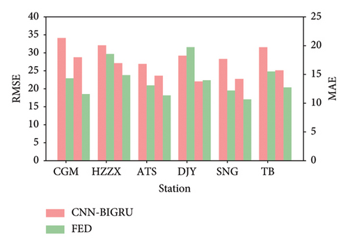
This reflects another advantage of FL: when there are few or missing data samples from one or some clients, FL collaborative training can use data from other clients to help learners train local models, greatly reducing the poor performance of the final prediction due to the lack of data samples from a client. In the same case, the traditional centralized model training method cannot use the data from other clients and is affected by the lack of data from a single client, so the trained model performance is often poor. The experimental comparison shows that the FL based collaborative training can greatly improve the generalization of the prediction model.
4.5. Comparative Experiment of FL Models
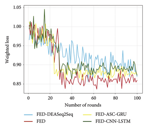
To demonstrate the effectiveness of the proposed FL-based subway passenger flow prediction model, FED, we conducted comparative experiments using three FL models: FED–DEASeq2Seq [25], FED–CNN–LSTM [26], and FED–ASC–GRU [27]. The experimental setup follows the specifications outlined in Section 4.2.
Figure 9 illustrates the convergence process of four FL models (FED, FED–ASC–GRU, FED–CNN–LSTM, and Weighted Loss) over 100 communication rounds, with the vertical axis representing the normalized loss value (where lower values indicate better performance) and the horizontal axis indicating the number of communication rounds. From Figure 9, it is evident that the FED model exhibits a significant advantage. In the initial stages, the differences in weighted loss values among the models are not very pronounced. However, as the rounds progress, the FED model demonstrates a distinct superiority. Its curve exhibits the most stable downward trend, allowing it to rapidly reduce the weighted loss value in fewer rounds compared to the other models, while exhibiting minimal fluctuations in later stages. This indicates that the FED model converges more quickly and efficiently reaches a relatively low loss level. Although the FED–DEASeq2Seq model also shows a downward trend, it experiences considerable fluctuations, indicating lower stability. The FED–ASC–GRU and FED–CNN–LSTM models initially have slower descent rates and struggle to further reduce loss values in the later stages. The rapid convergence and stability of the FED model suggest that it can learn the patterns and regularities in the data more quickly and accurately for subway passenger flow prediction tasks, thereby reducing prediction errors and providing more reliable passenger flow forecasts for subway operational management.
4.6. Discuss the Necessity of Pretraining
Since the parameters in the initial global model are randomly generated by the server, this also leads to relatively low performance and difficulty in convergence of the initial model. It may even affect the final result when the number of communication rounds is not enough. In response to this situation, this paper further discusses the steps of pretraining the model to the server before iteration. In general, pretraining refers to the method of training an initial model using a portion of the total historical data as pretraining data. However, this paper considers that clients with large amounts of data have a significant impact on the final model. Therefore, we only select the same amount of data as pretraining data for each client. This can minimize the excessive impact of clients with large amounts of data on the final result. Taking Shenzhen Metro Lines 1, 2, and 3 as three local clients, the data of inbound passenger flow at two transfer stations on each line on weekdays are selected for experimentation. The number of FL communication rounds is set as 50, and the pretraining data are the inbound passenger flow data of each station for six working days. Two FL methods, pretraining and no pretraining, are used to make multistep prediction, respectively. The results are compared as shown in Figure 10.
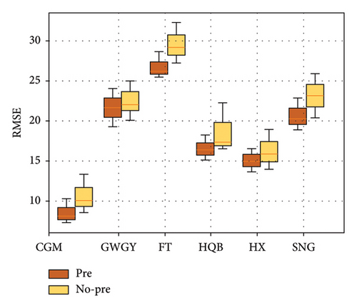
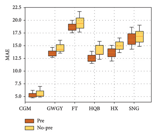
Figure 10 systematically compares the impact of pretraining strategies on multisite subway passenger flow prediction performance within a FL framework using two metrics: RMSE (Figure 10(a)) and MAE (Figure 10(b)). The experiments selected six key stations from Shenzhen Metro Lines 1, 2, and 3 (MAF, CCM, GWGY, FT, HQB, HX, and SNG), representing different functional scenarios such as commuting hubs, commercial areas, and transfer stations. The results indicate that the pretrained model significantly outperformed the nonpretrained model across all stations, with a notable reduction in volatility for multistep predictions. For instance, using RMSE as an example (Figure 10(a)), the pretrained group exhibited a prediction error of 10.2 at SNG station (commuting hub), which is a 35.4% reduction compared to the nonpretrained group (15.8). At HX Station (commercial area), where passenger flow fluctuates significantly, pretraining reduced RMSE from 18.3 to 13.7 (a decrease of 25.1%). This demonstrates that pretraining effectively mitigated the negative impact of data heterogeneity on the model’s generalization capability by balancing the initial parameters. The MAE metric (Figure 10(b)) further corroborates this trend, showing that the pretrained model achieved an MAE of 7.5 at CCM station (transfer station), a 33.0% reduction compared with the nonpretrained group (11.2). In addition, the error distribution became more concentrated, with the standard deviation decreasing from 2.8 to 1.6, indicating enhanced adaptability of the model to sudden increases in passenger flow.
Notably, pretraining significantly improved the stability of multistep predictions. For instance, at GWGY station (tourist hotspot), the RMSE for the nonpretrained model increased from 12.4 in the first step to 21.7 in the sixth step (an increase of 75.0%), while the RMSE for the pretrained model only rose from 9.8 to 14.3 (an increase of 45.9%), reflecting a 38.8% reduction in error accumulation rate. This improvement stems from the prior spatiotemporal feature extraction capability endowed by pretraining; the initial parameters encoded common patterns across stations (such as the periodicity of peak hours), facilitating faster convergence to the global optimum during federated iterations and reducing local oscillations caused by initial randomness. Statistical tests indicated that the RMSE differences between the pretrained and nonpretrained groups at all stations were significant (paired t-test, p < 0.01), with the most notable differences observed at HQB station (p = 0.002) and FT station (p = 0.001), confirming the strong adaptability of the pretraining strategy for complex stations (e.g., multiline transfers).
In addition, pretraining effectively balanced the influence of clients. In the absence of pretraining, the dominance of data-rich SNG Station (average daily passenger flow of 120,000) resulted in inflated prediction errors for other stations (such as MAF station, RMSE = 14.5). However, pretraining enforced equivalence in data sampling, reducing MAF station’s RMSE to 10.8 (a decrease of 25.5%) and narrowing the performance gap among the stations (RMSE range) from 8.7 to 4.9. This indicates that pretraining curbed the phenomenon of “data hegemony” and enhanced the fairness of the federated framework.
4.7. Actual Application Value
Combining the characteristics of CNN–BIGRU and FL, we believe that the method proposed in this paper has significant potential applications in the following real-world scenarios.
4.7.1. Short-Term Passenger Flow Management in Multisite Urban Rail Transit Systems
Traditional passenger flow forecasting methods typically require aggregating all data at a central server for unified analysis, which not only poses significant privacy risks but also consumes substantial communication resources. In contrast, our method incorporates a FL mechanism to enable distributed collaborative modeling across different stations or urban areas. In addition, passenger flow data in urban rail transit often include sensitive information such as passengers’ departure locations, destinations, and travel times. By using FL, we can avoid uploading raw data to a central server, thus protecting user privacy. Leveraging the efficient modeling capabilities of CNN–BIGRU, our approach can capture the dynamic characteristics of passenger flow in real-time and provide timely predictions, assisting operational departments in dynamically adjusting transportation plans.
4.7.2. Passenger Diversion Management in Integrated Transportation Hubs
In major transportation hubs such as airports and high-speed rail stations, passenger flow is often highly variable and influenced by external factors such as weather and flight/train schedules. Our method facilitates cross-system collaborative modeling by integrating distributed data from various transportation subsystems (such as subways, buses, and taxis) through a FL framework, establishing comprehensive passenger flow prediction models to better analyze distribution patterns across different modes of transport. By optimizing transfer resource allocation, we can dynamically adjust waiting areas, ticketing channels, and related service facilities after predicting passenger flow distribution during peak periods, thereby improving transfer efficiency.
4.7.3. Distributed Deployment on Edge Devices
Given that the CNN–BIGRU model proposed in this study has a relatively low computational burden and the FL framework supports distributed deployment, our method can run on edge devices within traffic management systems (such as station servers or local terminals at transportation hubs). This approach eliminates the delays associated with uploading data to a central server, resulting in more timely predictions. The model’s lightweight structure, particularly the design of BIGRU compared with LSTM, makes it suitable for use in resource-constrained environments, such as metro stations or mobile dispatch terminals.
4.7.4. Enhancing Operational Efficiency of Transportation Systems
By providing high-precision short-term passenger flow forecasts, our method enables refined operations in train scheduling, resource allocation, and station management, reducing resource waste and enhancing passenger satisfaction. For instance, when a significant increase in passenger flow is predicted for a specific route or station during peak periods, we can proactively increase train frequencies or deploy additional staff. Conversely, during off-peak periods, the frequency of train departures can be appropriately reduced based on forecast results, thereby lowering operational costs.
4.7.5. Improving Passenger Experience
Alleviating congestion during peak periods and reducing passenger wait times are crucial for enhancing the travel experience. Our method, through accurate forecasting of peak passenger flow and distribution, can assist traffic management authorities in developing more optimized diversion plans. For example, we can release prediction information in advance to encourage passengers to stagger their travel times or plan more optimal transfer routes. Furthermore, optimizing the distribution of waiting areas or automatic ticket machines based on forecast results can help reduce queue times.
4.7.6. Supporting Smart City Development
Our method, which integrates privacy-preserving FL mechanisms, serves as a reference model for large-scale traffic data analysis within smart cities, thereby supporting safer and more sustainable transportation management strategies. It enables data collaboration across different modes of transportation (such as subways, buses, and shared bicycles), facilitating comprehensive management of multimodal transportation systems and providing theoretical and technical support for future automated traffic scheduling systems.
5. Conclusion
This paper introduces FL as an innovative method for collaborative model training, aimed at addressing several key challenges: the insufficient quantity and features of subway passenger flow data, the poor generalization capabilities of existing prediction models, and the high privacy concerns associated with subway passenger data [21]. We propose a short-term passenger flow prediction method based on FL, which first constructs a CNN–BIGRU model. This model utilizes convolutional calculations via CNN to extract features from subway passenger flow data, while the BIGRU captures long-term dependencies from past to future, allowing for the learning of dynamic changes in passenger flow at subway stations. Our approach employs joint learning and collaborative training, replacing traditional centralized model training methods. This effectively mitigates the need to transmit large volumes of data over the network, thereby safeguarding data privacy. Notably, the method still achieves superior prediction performance even in scenarios with limited single-point data. We tested the predictive effectiveness of FL using small sample data and discussed the necessity of model pretraining, demonstrating its importance in enhancing prediction performance.
However, our current study has certain limitations, primarily in the following areas: first, due to the high privacy concerns surrounding subway passenger flow data, we were only able to access the dataset from Shenzhen Metro, which restricts validation across a broader range of subway datasets and impacts the generalization ability of our short-term passenger flow prediction method. Second, the Shenzhen Metro dataset was collected solely from smart card data, which may result in incomplete data. Lastly, this study focuses exclusively on the analysis and prediction of subway passenger flow data, without considering other potentially influential factors such as weather changes and significant events.
In light of these limitations, future research will focus on the following directions. (1) Optimizing communication efficiency in FL: we will explore strategies to enhance communication efficiency by compressing model parameters, reducing communication frequency, and utilizing efficient transmission protocols. In addition, we will consider the application of model pruning and quantization techniques to lessen communication burdens and improve overall performance. (2) Enhancing model adaptability to non-IID data: we aim to discuss the design of more robust algorithms to address discrepancies in data distribution across different subway lines or regions. This will include exploring adaptive optimization techniques, methods of ensemble learning, and the introduction of more flexible aggregation strategies to improve the model’s predictive capabilities when dealing with non-IID data. (3) Integrating more external factors (such as weather and events): we will incorporate external factors such as weather changes and significant events into the model’s input features. This will involve methodologies for data acquisition and feature extraction. By leveraging time series analysis and feature engineering techniques, we aim to enhance the model’s sensitivity and adaptability to various external influences.
Ethics Statement
This study does not violate any ethical standards.
Disclosure
A preprint has previously been published [36].
The authors acknowledge that an earlier version of this manuscript was posted as a preprint on Research Square and can be accessed at the following link: https://papers.ssrn.com/sol3/papers.cfm?abstract_id=4403252.
Conflicts of Interest
The authors declare no conflicts of interest.
Author Contributions
Guowen Dai: coding, methodology, modeling, and paper writing. Jinjun Tang: conceptualization and reviewing and editing. Jie Zeng: data preprocessing. Yuting Jiang: text correction. All authors reviewed the manuscript.
Funding
This research was funded in part by the Key R&D Program of Hunan Province (Grant no. 2023GK2014), the National Natural Science Foundation of China (Grant no. 52172310), the Transportation Science and Technology Plan Project of Shandong Transportation Department (Grant no. 2022B62), the Key Technology Projects in the Transportation Industry (Grant no. 2022-ZD6-077), Shandong Provincial Natural Science Foundation (Grant no. ZR20210F137), Central South University Graduate Student Independent Exploration and Innovation Project (Grant no. 2023ZZTS0340), and Fundamental Research Funds for the Central Universities of Central South University (Grant no. 2025ZZTS0107).
Appendix A: Notation
When simulating a federated architecture with a single device, the total training time increases linearly with the number of clients, but asynchronous aggregation strategy can reduce waiting latency by 15%. The RTX 3070 GPU has a memory usage rate of only 76% (peak of 6.2/8 GB), indicating that the model supports scaling to larger sizes or more complex structures.
| Abbreviation | Description |
|---|---|
| BAZX | Bao An Zhong Xin |
| CGM | Che Gong Miao |
| GS | Guang Sha |
| GWGY | Gou Wu Guang Chang |
| HZZX | Hui Zhan Zhong Xin |
| LJ | Lao Jie |
| QHW | Qian Hai Wan |
| ATS | An Tuo Shan |
| DJY | Da Ju Yuan |
| FT | Fu Tian |
| GSB | Gang Sha Bei |
| HH | Hou Hai |
| HQB | Hua Qiang Bei |
| HBL | Huang Bei Ling |
| JT | Jing Tian |
| SJZC | Shi Jie Zhi Chaung |
| SMZX | Civic Center |
| HL | Hong Ling |
| HX | Hua Xin |
| LHC | Lian Hua Village |
| SNG | Shao Nian Gong |
| SS | Shi Sha |
| TB | Tian Bei |
| TXL | Tong Xin Ling |
| Task phase | Average time consumption (per round) (s) | GPU memory usage peak (GB) |
|---|---|---|
| Client local training | 78 | 6.2 |
| Server global aggregation | 12 | 1.1 |
| Abbreviation | Full name |
|---|---|
| CNN | Convolutional neural network |
| BIGRU | Bidirectional gated recurrent unit |
| FL | Federated learning |
| RMSE | Root mean square error |
| MAE | Mean absolute error |
| BIRNN | Bidirectional recurrent neural network |
| SVR | Support vector regression |
| LSTM | Long short-term memory |
| BILSTM | Bidirectional long short-term memory |
| BP | Back propagation |
Open Research
Data Availability Statement
The data that support the findings of this study are available from the corresponding author upon reasonable request.


