Volume 2025, Issue 1 6659119

Research Article

Open Access

Modeling to Engineering and Failure Times Data: Using the Marshall–Olkin Extended Exponential Distribution

Ibrahim E. Ragab

orcid.org/0000-0001-6087-8649

Department of Basic Sciences , Egyptian Institute of Alexandria Academy for Management and Accounting , EIA , Alexandria , 21919 , Egypt , eia.edu.eg

Search for more papers by this author

Najwan Alsadat,

Najwan Alsadat

orcid.org/0000-0001-8884-8281

Department of Quantitative Analysis , College of Business Administration , King Saud University , P.O. Box 71115, Riyadh , 11587 , Saudi Arabia , ksu.edu.sa

Search for more papers by this author

Mustapha Muhammad,

Mustapha Muhammad

Department of Mathematics , Guangdong University of Petrochemical Technology , Maoming , China , gdpa.edu.cn

Search for more papers by this author

Suleman Nasiru,

Corresponding Author

Suleman Nasiru

[email protected]

orcid.org/0000-0001-6652-4251

Department of Statistics and Actuarial Science , School of Mathematical Sciences , C. K. Tedam University of Technology and Applied Sciences , Navrongo , Ghana , cktutas.edu.gh

Search for more papers by this author

Mohammed Elgarhy,

Mohammed Elgarhy

orcid.org/0000-0002-1333-3862

Department of Basic Sciences , Higher Institute for Administrative Sciences , Belbeis , AlSharkia , Egypt

Search for more papers by this author

Ibrahim E. Ragab,

Ibrahim E. Ragab

orcid.org/0000-0001-6087-8649

Department of Basic Sciences , Egyptian Institute of Alexandria Academy for Management and Accounting , EIA , Alexandria , 21919 , Egypt , eia.edu.eg

Search for more papers by this author

Najwan Alsadat,

Najwan Alsadat

orcid.org/0000-0001-8884-8281

Department of Quantitative Analysis , College of Business Administration , King Saud University , P.O. Box 71115, Riyadh , 11587 , Saudi Arabia , ksu.edu.sa

Search for more papers by this author

Mustapha Muhammad,

Mustapha Muhammad

Department of Mathematics , Guangdong University of Petrochemical Technology , Maoming , China , gdpa.edu.cn

Search for more papers by this author

Suleman Nasiru,

Corresponding Author

Suleman Nasiru

[email protected]

orcid.org/0000-0001-6652-4251

Department of Statistics and Actuarial Science , School of Mathematical Sciences , C. K. Tedam University of Technology and Applied Sciences , Navrongo , Ghana , cktutas.edu.gh

Search for more papers by this author

Mohammed Elgarhy,

Mohammed Elgarhy

orcid.org/0000-0002-1333-3862

Department of Basic Sciences , Higher Institute for Administrative Sciences , Belbeis , AlSharkia , Egypt

Search for more papers by this author

First published: 14 July 2025

https://doi.org/10.1155/admp/6659119

Academic Editor: Shikha Binwal

Share a link

Email
Wechat
Bluesky

Abstract

In this article, we study and introduce the Marshall–Olkin extended exponential (MO-ExE) distribution, a novel three-parameter life expectancy distribution. The new model is characterized by high adaptability in data analysis. Various mathematical properties, including ordinary moments, moment-generating functions (MGFs), and conditional moments (CMs) of the new suggested model, were computed. The model parameters are estimated using the maximum likelihood method. A simulation study is evaluated to demonstrate the behavior of the parameter model. In the final analysis, we demonstrate the significance of the novel model by examining practical data applications, thus, showing the adaptability and potential of the MO-ExE model.

1. Introduction

The application of distribution theory is crucial for modeling lifetime data in the life insurance industry and other areas such as reliability, queueing theory, and related topics. The exponential distribution is a well-known continuous probability model in life insurance, reliability engineering, and survival analysis. The aforementioned statistical distribution is used extensively regarding reliability issues and other applications. The wide application of the exponential distribution, even in improper situations, is undeniably due to its simplicity. Nevertheless, the exponential distribution has the problem of a constant failure/hazard rate, which makes it unsuitable for representing data sets of many complicated life phenomena that may have ascending, descending, or cyclic patterns. We propose to extend the exponential distribution to improve its applicability in the area of reliability. The exponential distribution has already been modified several times to increase its versatility. These modifications include the exponentiated exponential (EE) distribution [1], the generalized exponential distribution [2], the inverted exponential distribution [3], and others. The exponential distribution significantly limits its ability to represent data sets derived from many complex events with nonconstant hazard rate function (HRF). This limitation arises from the inherent property of the exponential distribution to assume a constant HRF. Numerous scientists have proposed various extensions of this theoretical structure. In [4], an additional extension of the exponential distribution, the extended exponential (ExE) distribution, was presented, and it can be used as an alternative to the distributions mentioned above. The cumulative distribution function (CDF) is provided via:

()

The probability density function (PDF) corresponding to Equation (1) is provided by:

()

Numerous authors have been inspired to produce more flexible and broad variations of the exponential distribution by its simplicity, memoryless characteristic, and constant hazard rate. These extended forms may be equivalent to actual data sets that demonstrate decreasing, growing, bathtub, decreasing-increasing, and unimodal failure rates. These failure rates are common in a variety of relevant disciplines, including engineering, medical, and reliability. Several notable extended forms of the exponential model are referred to as Harris ExE [5], sine generalized linear exponential [6], transmuted generalized exponential [7], type II Topp–Leone inverse length biased exponential [8], alpha power exponential [9, 10], unit ExE [11], Kumaraswamy transmuted exponential [12], Kavya–Manoharan generalized exponential [13], modified exponential [14], half logistic modified Kies exponential [15], Marshall–Olkin (MO) logistic exponential [16], Kavya–Manoharan inverse length biased exponential [17], Burr-X EE [18], Kavya–Manoharan Kumaraswamy exponential [19], and MO alpha power exponential [20]. For more information see [21–24].

Marshall and Olkin [25] proposed a general method of adding a new positive shape parameter

to a baseline distribution yielding the MO extended-G distribution. The survival function (SF) of the MO extended-G distribution is defined as:

()

The resulting CDF and PDF of the MO extended-G distribution are, respectively, given by:

()

and

()

where G(x) and g(x) represent the CDF and PDF of the baseline random variable X with vector parameter η. The corresponding HRF is derived as:

()

where

is the SF of the baseline random variable.

Several authors have recently applied their methodology to extend the known distribution areas. Ghitany et al. [26] presented MO extended Weibull distribution, Saboor and Pogány [27] proposed MO gamma-Weibull distribution, Krishna et al. [28] studied the MO Fréchet distribution, Cordeiro and Lemonte [29] investigated the MO extended Weibull distribution, Cordeiro et al. [30] provided the MO family of distributions, Alabdulhadi et al. [31] studied some statistical inference of MO-ExE distribution, Alsadat et al. [32] proposed MO Weibull–Burr XII distribution, Okorie et al. [33] discussed MO generalized Erlang-truncated exponential distribution, MirMostafaee et al. [34] studied MO extended generalized Rayleigh distribution, Afify et al. [35] presented the MO additive Weibull distribution, Gilliarose and Tomy [36] introduced MO extended power Lomax distribution, Nwezza and Ugwuowo [37] proposed the MO Gumbel–Lomax distribution, Afify et al. [38] studied MO odd Burr III-G family of distributions, Elbatal and Elgarhy [39] discussed extended MO length-biased exponential distribution, and Haq et al. [40] proposed MO power Lomax distribution, among others.

In this study, we adopt the ExE distribution as the baseline distribution, introducing a new form of the MO model. The MO-ExE distribution is the model that results from transforming the ExE distribution using the MO transformation. The MO-ExE model is sufficiently motivated to be investigated by the following reasons. It is expressed as specified below:

•
The MO-ExE distribution gives more flexibility than some well-known statistical models for engineering and failure times data as we illustrate in Section 6.
•
The MO-ExE distribution is highly adaptable and includes three submodels.
•
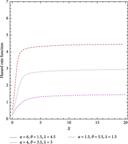
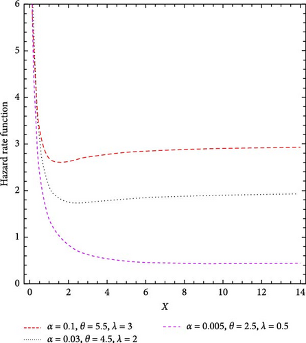
The shapes of the PDF for the MO-ExE distribution can be decreasing, right skewness, and unimodal. However, its HRF can be decreasing or increasing.
•
Various statistical and mathematical features of the MO-ExE distribution are computed.
•
The parameters of the MO-ExE distribution are estimated utilizing maximum likelihood approach.

The remainder of the paper is structured as follows: The MO-ExE distribution and the proposed model’s plots of the PDF and HRF are defined in Section 2. Section 3 discusses a number of mathematical features. We present the maximum likelihood estimates (MLEs) of the unknown parameters in Section 5. In Section 6, we ultimately demonstrate the significance of the new model by an examination of real-world data applications, illustrating its adaptability and potential, Finally, some concluding remarks are presented in Section 7.

2. The MO-ExE Distribution

This section explains the key concepts of the MO-ExE distribution, including the PDF, CDF, and HRF, accompanied by visual representations of the PDF and HRF. The CDF and PDF are derived by substituting Equations (1) and (2) into Equations (4) and (5), leading to the following formulation:

()

where α, θ, and λ are three scale parameters. The corresponding PDF is given by:

()

Henceforth, let X ∼MO-ExE(ϕ) having PDF (8), where ϕ = (α, θ, λ) is the set of parameters. The MO-ExE distribution is composed of three submodels.

1.
The MO-ExE distribution leads to the ExE distribution when α = 1.
2.
The MO-ExE distribution leads to the ExE distribution when α = 1 and θ = 0.
3.
The MO-ExE distribution leads to the MO-exponential distribution when θ = 0.

The HRF for the MO-ExE distribution is calculated as follows:

()

Figure 1 displays the PDF plots of the MO-ExE distribution for specific parameter values ϕ = (α, θ, λ), demonstrating that the proposed model’s PDF is positively skewed, unimodal, and monotonically decreasing.

Details are in the caption following the image — **Figure 1 (a)**
Open in figure viewer PowerPoint

(a, b) Plots of the MO-ExE density function for different parameter values.

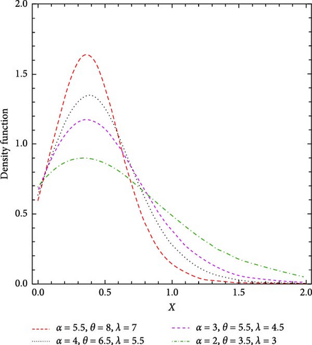
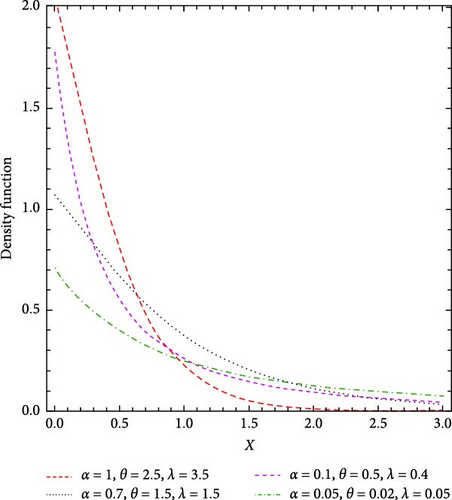
Figure 2 shows the HRF patterns corresponding to different distribution parameter values. The HRF of the MO-ExE distribution can be increasing or decreasing.

2.1. Useful Expansion for the PDF

This subsection looks at essential PDF expansions for the proposed model in order to determine its statistical properties. The generalized binomial theorem is expressed as follows:

()

where |z| < 1 and k > 0 are real noninteger values.

Using Equation (10), the PDF (8) can be reformulated as:

applying the binomial expansion to the last term of the previous equation, yields:

()

where

3. Statistical Properties

This section examines the fundamental distributional characteristics of the MO-ExE model, including moments, moment-generating functions (MGFs), conditional moments (CMs), mean deviation, and the Lorenz and Bonferroni curves, as well as residual and inverted residual life functions.

3.1. Ordinary Moments

Ordinary moments are statistical metrics that yield valuable insights into the distribution of product lifetimes, which is essential for assessing reliability and upholding quality standards. Additionally, they serve as indicators of failure rates for systems and components, facilitating maintenance scheduling and contributing to the enhancement of overall reliability. The r^th moment of MO-ExE distribution can be obtained by the following:

()

where

denotes the gamma function.

The abovementioned Equation (12) serves as an essential tool for deriving the first-four moments:

•
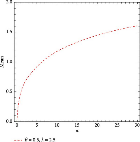
First moment: Mean is the average value of a distribution, representing the central point of all data.
•
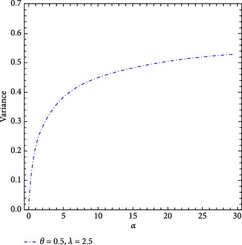
Second moment: Variance measures the dispersion of data points from the mean, indicating the spread of values.
•
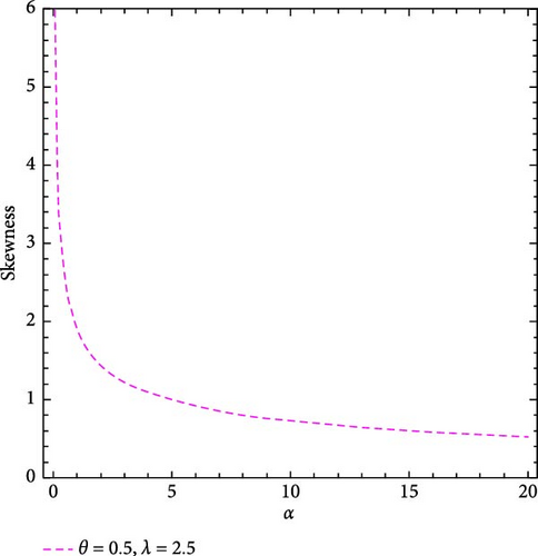
Third moment: Skewness reflects the distribution’s asymmetry. A positive skew denotes a longer right tail, while a negative skew indicates a longer left tail.
•
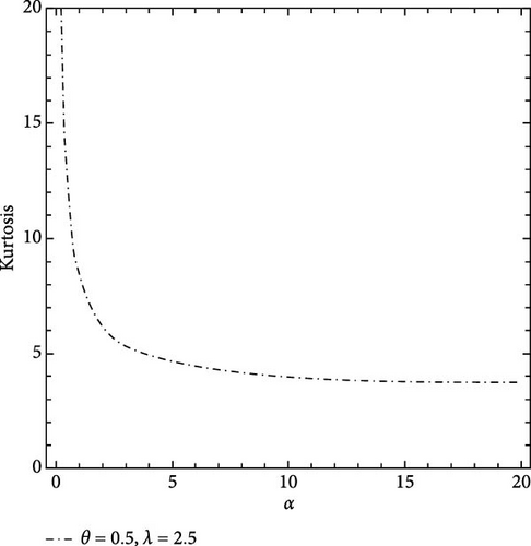
Fourth moment: Kurtosis [τ₂ = (μ₄ − 4μ μ₃ + 6μ²μ₂ − 3μ⁴)/σ⁴] describes the “peakedness” of a distribution. High kurtosis indicates a sharp peak, whereas low kurtosis suggests a flatter distribution.

In addition, the coefficient of variation [CV = σ/μ] quantifies the relative spread of data around the mean, analyzing these moments provides valuable insights into the shape and spread of the distribution, aiding informed decision-making based on the data.

Table 1 provides a comprehensive analysis of the first four moments of the MO-ExE distribution across various parameter values (λ, θ), maintaining a constant parameter value of α = 0.5. It is significant to note that higher parameter values are associated with a decrease in both the mean and variance. Conversely, skewness, kurtosis, and the coefficient of variation exhibit an increasing trend. Figure 3 provides a visual representation of these findings.

Table 1. The first four moments’ numerical values and CV for the MO-ExE distribution (α = 0.5).

θ	λ ↑				↓	σ² ↓	τ₁ ↑	τ₂ ↑	CV ↑
θ = 0.5	1	0.9373	1.9726	6.5292	29.2297	1.0940	2.2980	10.7225	1.1158
	1.5	0.5825	0.7841	1.6849	4.9341	0.4449	2.3926	11.4155	1.1451
	2	0.4182	0.4104	0.6483	1.4028	0.2355	2.4482	11.8510	1.1604
	2.5	0.3247	0.2497	0.3107	0.5315	0.1442	2.4836	12.1410	1.1694
	3	0.2648	0.1670	0.1711	0.2415	0.0968	2.5075	12.3433	1.1751
	3.5	0.2233	0.1192	0.1036	0.1244	0.0693	2.5245	12.4898	1.1790
	4	0.1929	0.0892	0.0673	0.0702	0.0520	2.5369	12.5994	1.1817

θ = 1	1	1.0704	2.4026	8.2487	37.8334	1.2570	2.1189	9.5538	1.0475
	1.5	0.6597	0.9522	2.1367	6.4503	0.5169	2.2238	10.2167	1.0898
	2	0.4687	0.4931	0.8162	1.8269	0.2735	2.2980	10.7225	1.1158
	2.5	0.3603	0.2965	0.3870	0.6860	0.1667	2.3521	11.1116	1.1331
	3	0.2912	0.1960	0.2106	0.3084	0.1112	2.3926	11.4155	1.1451
	3.5	0.2437	0.1384	0.1261	0.1571	0.0791	2.4237	11.6567	1.1538
	4	0.2091	0.1026	0.0810	0.0877	0.0589	2.4482	11.8510	1.1604

θ = 1.5	1	1.1541	2.6699	9.3036	43.0637	1.3380	2.0248	9.0094	1.0023
	1.5	0.7136	1.0678	2.4441	7.4733	0.5587	2.1189	9.5538	1.0475
	2	0.5062	0.5540	0.9383	2.1331	0.2978	2.1930	10.0153	1.0781
	2.5	0.3879	0.3325	0.4451	0.8030	0.1820	2.2514	10.4007	1.0998
	3	0.3124	0.2192	0.2418	0.3609	0.1216	2.2980	10.7225	1.1158
	3.5	0.2605	0.1542	0.1444	0.1834	0.0863	2.3358	10.9927	1.1280
	4	0.2227	0.1138	0.0924	0.1021	0.0642	2.3668	11.2211	1.1376

θ = 2	1	1.2117	2.8523	10.0171	46.5801	1.3841	1.9694	8.7115	0.9710
	1.5	0.7532	1.1524	2.6668	8.2102	0.5850	2.0505	9.1529	1.0155
	2	0.5352	0.6007	1.0311	2.3646	0.3142	2.1189	9.5538	1.0475
	2.5	0.4101	0.3612	0.4909	0.8947	0.1930	2.1761	9.9075	1.0714
	3	0.3299	0.2380	0.2671	0.4031	0.1292	2.2238	10.2167	1.0898
	3.5	0.2746	0.1673	0.1595	0.2051	0.0919	2.2640	10.4866	1.1042
	4	0.2343	0.1233	0.1020	0.1142	0.0684	2.2980	10.7225	1.1158

θ = 2.5	1	1.2537	2.9846	10.5319	49.1066	1.4128	1.9340	8.5302	0.9481
	1.5	0.7837	1.2169	2.8356	8.7663	0.6027	2.0033	8.8917	0.9906
	2	0.5582	0.6376	1.1041	2.5458	0.3259	2.0651	9.2368	1.0227
	2.5	0.4281	0.3844	0.5279	0.9685	0.2011	2.1189	9.5538	1.0475
	3	0.3444	0.2537	0.2880	0.4379	0.1351	2.1655	9.8405	1.0671
	3.5	0.2865	0.1784	0.1722	0.2233	0.0963	2.2057	10.0981	1.0830
	4	0.2444	0.1314	0.1102	0.1245	0.0717	2.2407	10.3291	1.0960

θ = 3	1	1.2858	3.0850	10.9209	51.0098	1.4318	1.9099	8.4113	0.9307
	1.5	0.8078	1.2677	2.9680	9.2010	0.6152	1.9694	8.7115	0.9710
	2	0.5770	0.6675	1.1630	2.6915	0.3345	2.0248	9.0094	1.0023
	2.5	0.4432	0.4037	0.5585	1.0292	0.2073	2.0747	9.2917	1.0272
	3	0.3568	0.2670	0.3055	0.4671	0.1397	2.1189	9.5538	1.0475
	3.5	0.2968	0.1879	0.1830	0.2388	0.0998	2.1582	9.7948	1.0641
	4	0.2531	0.1385	0.1173	0.1333	0.0744	2.1930	10.0153	1.0781

3.2. MGF

The MGF serves as an essential instrument for evaluating the distributions of sums of random variables, and it offers a distinctive methodology for deriving analytical results that is independent of traditional probability or CDFs. The MGF of MO-ExE is given as follows:

()

The MGF serves as essential instruments in the fields of quality and reliability engineering, environmental sciences, and wireless communications, providing a robust mathematical framework for the analysis and interpretation of diverse datasets.

3.3. Incomplete Moments (IMOs)

The IMOs augment traditional moments by offering more profound insights into the distribution of a random variable, particularly in targeted regions. In the context of survival analysis, IMOs are employed to investigate the duration until an event of interest, such as the recurrence of a disease, transpires within a defined timeframe. If a random variable X follows the MO-ExE distribution, the s^th IMOs can be determined using the following equation:

()

where

is the lower incomplete gamma function.

A commendable application of IMOs is to evaluate the average absolute deviation of observations relative to their mean (or median). The mean deviation about the mean (or the median) are given, respectively, by:

and

Utilizing Equation (12), we obtain the mean . The value of is determined from Equation (7), whereas the first IMO () is calculated from Equation (14) with s = 1.

3.4. CMs

The CMs offer valuable insights into the behavior of random variables under specific conditions. By examining these moments, we gain a deeper understanding of how variables respond in particular scenarios, enhancing our comprehension beyond standard distribution analysis. This approach is especially useful for identifying nuanced patterns and relationships within data. CMs have wide-ranging applications, particularly in economics, finance, and machine learning, where grasping conditional behaviors is essential for informed decision-making and predictions. The CMs of the MO-ExE distribution are detailed as follows:

()

where

is the upper incomplete gamma function.

3.5. Mean Residual Life (MRL)

The MRL represents a pivotal concept within the realms of reliability theory and survival analysis, signifying the expected remaining lifespan of an item or individual that has already surpassed a specified point in time (t). This metric holds significant importance for assessing future system reliability and forecasting patient outcomes. The MRL for the MO-ExE distribution is given by:

where υ₁(t) represents the first CM derived by substituting n = 1 into Equation (14) yields:

()

3.6. Mean Inactivity Time (MIT)

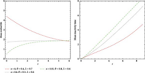
The MIT is a critical metric in reliability engineering that quantifies the average duration a system or component remains nonoperational prior to failure, necessitating repair or replacement. This metric is instrumental in improving reliability and optimizing maintenance scheduling practices. The MIT for the proposed model is provided via:

where ξ₁(t) is the first IMO obtained by substituting s = 1 into Equation (14) gives:

()

Table 2 illustrates the MRL and MIT of the MO-ExE distribution at t = 0.5, across a range of parameter values ϕ = (α, θ, λ), demonstrating that both functions display an increasing trend as the parameter values decrease. Furthermore, Figure 4 presents the distinct variations of MRL (on the right side) and MIT (on the left side).

Table 2. The MRL and MIT of the MO-ExE distribution (t = 0.5).

α ↓	θ ↓	λ ↓	MRL ↑	MIT ↑
15	4	5	0.22415	0.76441
7	3.5	4	0.28844	0.78969
5	3	3.5	0.33552	0.80111
2.5	2.5	3	0.39255	0.88581
0.7	1	1.5	0.78272	0.94841
0.3	0.6	1	1.07806	1.06569
0.1	0.4	0.5	1.73405	1.11882
0.01	0.2	0.1	3.49257	1.15238
0.005	0.01	0.05	4.49875	1.28239

3.7. Moments of the Residual and Reversed Residual Life

In this subsection, we will derive the n^th moment of the residual life and the reversed residual life using the following formula:

Utilizing the binomial expansion for the term (x − t)ⁿ and inserting PDF (11) into the abovementioned formula, leads to the following results:

()

Similarly, the n^th moment of the reversed residual life is given by:

()

4. Maximum Likelihood Estimation

This section describes the process for deriving the MLEs of the parameters associated to the MO-ExE distribution utilizing complete sample data. Let X₁, X₂, …, X_n be a random sample of size n from the MO-ExE(ϕ), where ϕ = (α, θ, λ)^T is the parameters vector, then, the log likelihood function is given by:

()

The score function is provided by:

Specifically, the components of the score vector are as follows:

()

and

()

The MLE of ϕ, say , is calculated by solving the nonlinear system U_n(ϕ) = 0. Analytical methods are insufficient for deriving solutions to these equations; however, statistical software as Wolfram Mathematica can employ iterative techniques to obtain numerical solutions.

5. Simulation Study

Monte Carlo simulation is an advanced computational technique that employs random sampling to approximate solutions to intricate mathematical problems. By systematically sampling from a probability distribution to generate random data points, this method effectively estimates distribution parameters. It proves particularly valuable in scenarios where deriving an exact analytical solution is challenging or unfeasible. Consequently, Monte Carlo simulation is extensively utilized in various fields, including finance, physics, and beyond, to evaluate complex systems or models. This study will use this method to analyze the estimate behavior of the proposed model and apply MLE for parameter estimation. Simulations and result analyses were conducted using Wolfram Mathematica (13). The estimators for the MO-ExE distribution were assessed through the simulation of cases: Case (I): (α = 0.5, θ = 2, λ = 1), Case (II): (α = 3, θ = 2.5, λ = 1.5), and Case (III): (α = 0.25, θ = 1.75, λ = 0.75).

A simulation study is undertaken involving the subsequent steps:

•
Generate 1000 random samples of sizes 100, 150, 200, 250, 300, 400, 500, and 600 from the MO-ExE distribution by employing the inverse CDF method applied to uniformly distributed random variables, as described in Equation (7).
•
Calculate the average of estimates from 1000 random samples using this relation:
•
Determine the average bias (BIAS) and mean squared error (MSE) of the estimates using the formulas:

The results obtained from the simulation study are displayed in Tables 3–5, which provide valuable insights. After analyzing these results, we can arrive at the following conclusion:

•
In the simulations, MLE estimates generally overestimate, except for the parameter θ in cases (I and III), and the parameter λ in case (II), which are underestimated.
•
The estimated values converge to the true values with an increasing sample size.
•
As the sample size increases, the absolute values of BIAS and MSE for the MLE decrease.
•
The MLE estimates’ BIAS and MSE approached zero as the sample size increases.

Table 3. Results of simulation study Case I: (α = 0.5, θ = 2, λ = 1).

Measures	n = 100	n = 150	n = 200	n = 250	n = 300	n = 400	n = 500	n = 600
α = 0.5	0.710152	0.668024	0.634878	0.630392	0.620537	0.602346	0.584785	0.573014
BIAS	0.210152	0.168024	0.134878	0.130392	0.120537	0.102346	0.084785	0.073014
MSE	0.217848	0.151064	0.118156	0.10487	0.096903	0.075671	0.059206	0.054452

θ = 2	1.76559	1.79623	1.83413	1.83574	1.83667	1.86413	1.88333	1.90290
BIAS	−0.23441	−0.20377	−0.16587	−0.16426	−0.16333	−0.13587	−0.11667	−0.09710
MSE	1.27486	1.15673	1.04817	1.02471	0.992976	0.910952	0.805603	0.731323

λ = 1	1.02536	1.01540	1.00889	1.00652	1.00658	1.00176	1.00143	1.000330
BIAS	0.025359	0.015402	0.008885	0.006518	0.006583	0.001763	0.001425	0.000330
MSE	0.051002	0.034367	0.0254	0.021492	0.017392	0.012844	0.010949	0.009074

Table 4. Results of simulation study Case II: (α = 3, θ = 2.5, λ = 1.5).

Measures	n = 100	n = 150	n = 200	n = 250	n = 300	n = 400	n = 500	n = 600
α = 3	3.81215	3.65019	3.64564	3.61889	3.57605	3.48971	3.48738	3.46129
BIAS	0.81215	0.65019	0.64564	0.61889	0.57605	0.48971	0.48738	0.46129
MSE	4.38468	3.11330	3.08591	2.61732	2.32387	1.86602	1.79911	1.65517

θ = 2.5	2.67899	2.67407	2.60746	2.59439	2.59066	2.58359	2.52955	2.50680
BIAS	0.17899	0.17407	0.10746	0.09439	0.09066	0.08359	0.02955	0.00680
MSE	3.24638	3.01471	2.98248	2.93237	2.78912	2.62994	2.54434	2.41234

λ = 1.5	1.47913	1.47948	1.48063	1.48229	1.48363	1.49407	1.49797	1.50053
BIAS	−0.02087	−0.02052	−0.01937	−0.01771	−0.01637	−0.00593	−0.00203	0.00053
MSE	0.03679	0.02539	0.02029	0.01742	0.01424	0.01111	0.01006	0.00903

Table 5. Results of simulation study Case III: (α = 0.25, θ = 1.75, λ = 0.75).

Measures	n = 100	n = 150	n = 200	n = 250	n = 300	n = 400	n = 500	n = 600
α = 0.25	0.38548	0.354444	0.330359	0.325346	0.318486	0.308585	0.294194	0.286468
BIAS	0.13548	0.104444	0.080359	0.075346	0.068486	0.058585	0.044194	0.036468
MSE	0.089257	0.058665	0.044311	0.038475	0.03493	0.028308	0.020041	0.017383

θ = 1.75	1.62622	1.65299	1.68664	1.69282	1.71127	1.72231	1.72544	1.73039
BIAS	−0.12378	−0.09701	−0.06336	−0.05718	−0.03873	−0.0276	−0.024559	−0.01961
MSE	1.17735	1.04847	0.918712	0.885921	0.839636	0.726631	0.626669	0.542414

λ = 0.75	0.788679	0.776316	0.764728	0.764814	0.762897	0.757914	0.756756	0.753474
BIAS	0.038679	0.026316	0.014728	0.014814	0.012897	0.007914	0.006756	0.003474
MSE	0.052833	0.035097	0.026013	0.021996	0.018097	0.01309	0.011444	0.009546

6. Applications

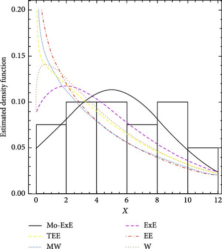
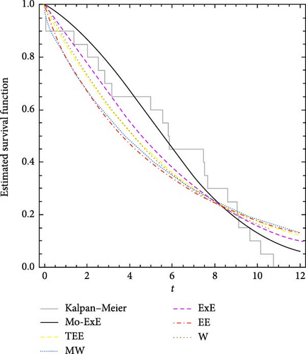
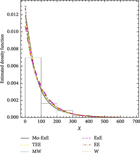
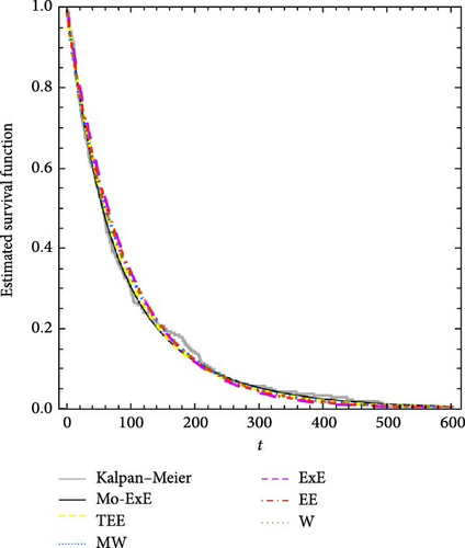
In this section, two examples from real life data are given for showing the adaptability of the suggested model in use. Proschan [41] established the first set of data, consisting of 213 observations on the breakdown of air conditioning units in 13 Boeing 720 jet aircraft. Murthy et al. [42]stated a second data set that comprised the failure times of 20 components during an incident. For each set of data, we examine the resulting fit of the MO-ExE distribution to other comparable lifespan models; namely transmuted EE (TEE) by Merovci [43], modified Weibull (MW) by Sarhan and Mazen [44], ExE, EE, and Weibull (W) [45].

For both datasets we estimate model parameters by applying the MLE method. We also examine the information criteria indicators (ICIs) according to parameter estimates, namely, Akaike’s ICI (C1), Bayesian ICI (C2), and Hannan–Quinn ICI (C3). In addition, the Anderson-Darling (C4), Cramér-von Mises (C5), Kolmogorov-Smirnov (C6) tests, including their p-values (C7) have been employed to evaluate the MO-ExE distribution’s goodness of fit to other comparable models; this measurement (C6) evaluates the fit between the empirical and fitted distribution functions, making it an effective tool for determining how well a random sample’s distribution matches the theoretical distribution. Overall, the model with the lowest score on these measures and the greatest p-value for the C6 statistic is regarded as the most efficient.

Tables 6–11 present the estimated MLEs and goodness-of-fit metrics for both data sets across competitor models. These indicators imply that the MO-ExE distribution is more competitive compared to other models, providing the best fit among them.

Table 6. The MLEs and their SEs in parenthesis for the failure data.

Model	Estimates
MO-ExE (α, θ, λ)	6.469230 (6.194090)	0.222574 (0.475727)	0.471253 (0.123832)
TEE (ϑ, ρ, λ)	−0.68938 (0.260644)	0.690760 (0.225134)	0.188114 (0.051126)
MW (δ, β, λ)	0.159586 (0.038955)	0.069382 (0.067450)	0.184692 (0.161200)
ExE (θ, λ)	0.298136 (0.060561)	0.701618 (0.787263)	—
EE (η, λ)	0.157018 (0.046738)	0.837733 (0.230045)	—
W (τ, λ)	0.146923 (0.072181)	1.08927 (0.220985)	—

Table 7. The C1, C2, and C3 metrics for the failure data.

Model	C1	C2	C3
MO-ExE	109.506	112.493	110.089
TEE	112.103	115.090	112.686
MW	111.663	114.650	112.246
ExE	110.901	112.892	111.289
EE	113.241	115.233	113.630
W	113.504	115.495	113.892

Table 8. The C4, C5, C6 and C7 metrics for the failure data.

Model	C4	C5	C6	C7
MO-ExE	1.08841	0.079026	0.146940	0.780878
TEE	1.46429	0.231952	0.217339	0.301264
MW	1.64430	0.313950	0.238784	0.204206
ExE	1.33735	0.159410	0.187678	0.481686
EE	1.96265	0.343900	0.249319	0.166324
W	1.49001	0.157713	0.222019	0.277692

Table 9. The MLEs and their SEs in parenthesis for the airplanes data.

Model	Estimates
MO-ExE (α, θ, λ)	0.19557 (0.124275)	0.0230811 (0.0166657)	0.00854864 (0.00203448)
TEE (ϑ, ρ, λ)	1.0151 (0.0833724)	0.508941 (0.234288)	0.0082095 (0.00148917)
MW (δ, β, λ)	3.59276 × 10⁻⁷ (0.016259)	0.015674 (0.017535)	0.924550 (0.097428)
ExE (θ, λ)	4.0143 × 10⁻⁶ (0.00132945)	0.0107404 (0.00151768)	—
EE (η, λ)	0.0102094 (0.000945646)	0.926924 (0.0830183)	—
W (τ, λ)	0.015674 (0.00391304)	0.924552 (0.0481744)	—

Table 10. The C1, C2, and C3 metrics for the airplanes data.

Model	C1	C2	C3
MO-ExE	2356.76	2366.85	2360.84
TEE	2358.53	2368.62	2362.61
MW	2361.17	2371.25	2365.24
ExE	2361.53	2368.25	2364.25
EE	2360.80	2367.53	2363.52
W	2359.17	2365.89	2361.89

Table 11. The C4, C5, C6, and C7 metrics for the airplanes data.

Model	C4	C5	C6	C7
Mo-ExE	0.360324	0.042783	0.038959	0.902942
TEE	0.650193	0.103808	0.044174	0.800182
MW	0.827545	0.127828	0.051952	0.613359
ExE	1.697890	0.324893	0.072620	0.211265
EE	1.201570	0.217023	0.064452	0.339115
W	12.66690	1.596710	0.124359	0.002753

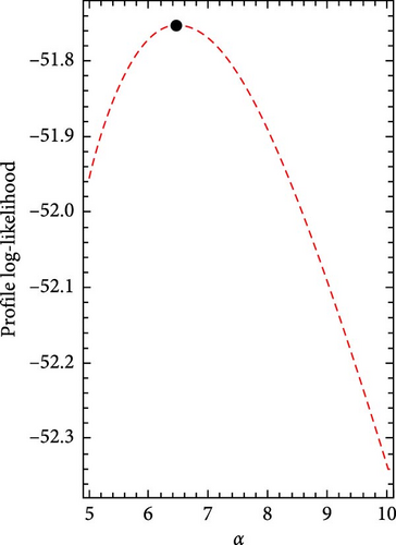
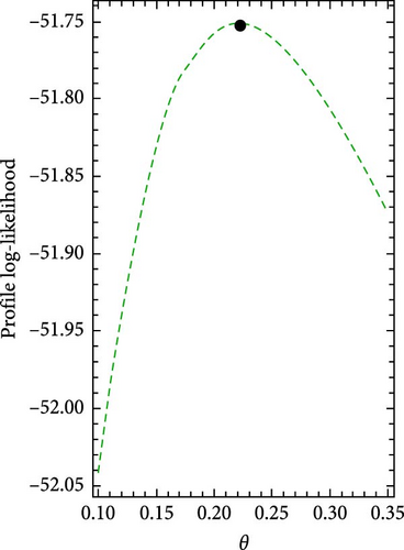
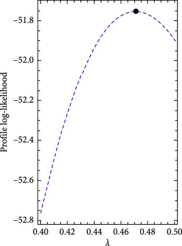
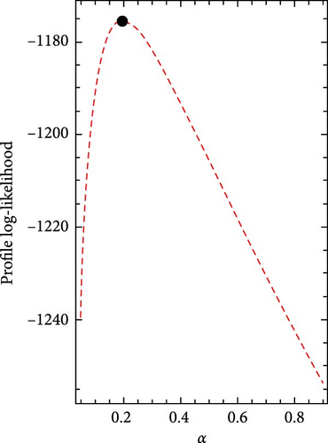
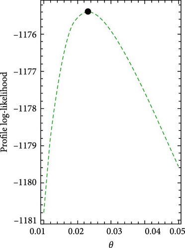
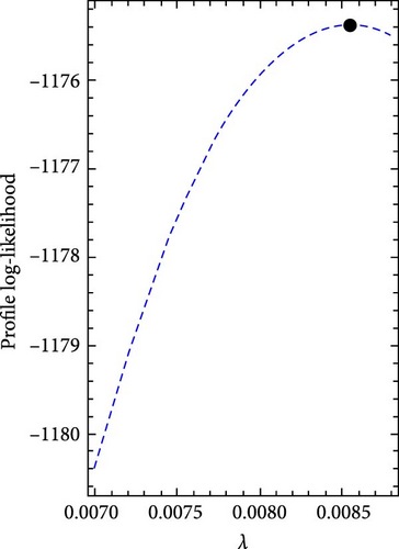
Figures 5 and 6 show the log-likelihood profiles, demonstrating that the likelihood formulas have a distinctive solution in regards to the distribution parameters. Moreover, Figures 7 and 8 illustrate the data sets’ histograms with the fitted PDF, as well as the empirical and estimated SF plots, to determine the MO-ExE model’s appropriateness.

7. Concluding Remarks

In this work, a novel three-parameter life expectancy distribution called the MO-ExE distribution is presented. The new model has a significant amount of data analysis versatility. Numerous mathematical features are examined in this work. The maximum likelihood method is used to estimate the model parameters. To show how the parameter model behaves, a simulation study is assessed. Finally, we show the versatility and potential of the innovative model by investigating real-world data applications, which emphasizes the model’s importance. The limitation of this article lies in the estimation part because we used the MLE method only with complete samples to estimate the parameters of the MO-ExE distribution. This limitation will open the door for researchers to estimate the parameters of the MO-ExE distribution using different estimation approaches using various ranked and censored schemes in future work.

Conflicts of Interest

The authors declare no conflicts of interest.

Funding

This research is supported by the Ongoing Research Funding Program (Grant ORF-2025-548), King Saud University, Riyadh, Saudi Arabia.

Acknowledgments

This research is supported by the Ongoing Research Funding Program (ORF-2025-548), King Saud University, Riyadh, Saudi Arabia.

Open Research

Data Availability Statement

The data that support the findings of this study are available upon request from the corresponding author. The data are not publicly available due to privacy or ethical restrictions.

References

1 Gupta R. D. and Kundu D., Exponentiated Exponential Family: An Alternative to Gamma and Weibull Distributions, Biometrical Journal. (2001) 43, no. 1, 117–130.
10.1002/1521-4036(200102)43:1<117::AID-BIMJ117>3.0.CO;2-R
Web of Science® Google Scholar
2 Gupta R. D. and Kundu D., Generalized Exponential Distribution: Existing Results and Some Recent Developments, Journal of Statistical Planning and Inference. (2007) 137, no. 11, 3537–3547, https://doi.org/10.1016/j.jspi.2007.03.030, 2-s2.0-34447510876.
10.1016/j.jspi.2007.03.030
Web of Science® Google Scholar
3 Keller A. Z., Kamath A. R. R., and Perera U. D., Reliability Analysis of CNC Machine Tools, Reliability Engineering. (1982) 3, no. 6, 449–473, https://doi.org/10.1016/0143-8174(82)90036-1, 2-s2.0-0020202738.
10.1016/0143-8174(82)90036-1
Web of Science® Google Scholar
4 Gómez Y. M., Bolfarine H., and Gómez H. W., A New Extension of the Exponential Distribution, Revista Colombiana de Estadística. (2014) 37, no. 1, 25–34, https://doi.org/10.15446/rce.v37n1.44355, 2-s2.0-84902459502.
10.15446/rce.v37n1.44355
Google Scholar
5 Pinho L. G. B., Cordeiro G. M., and Nobre J. S., The Harris Extended Exponential Distribution, Communications in Statistics—Theory and Methods. (2015) 44, no. 16, 3486–3502, https://doi.org/10.1080/03610926.2013.851221, 2-s2.0-84941092896.
10.1080/03610926.2013.851221
Web of Science® Google Scholar
6 Alotaibi N., Al-Moisheer A. S., Elbatal I., Elgarhy M., and Almetwally E. M., Bayesian and Non-Bayesian Analysis for the Sine Generalized Linear Exponential Model under Progressively Censored Data, Computer Modeling in Engineering & Sciences. (2024) 140, no. 3, 2795–2823, https://doi.org/10.32604/cmes.2024.049188.
10.32604/cmes.2024.049188
Web of Science® Google Scholar
7 Khan M. S., King R., and Hudson I. L., Transmuted Generalized Exponential Distribution: A Generalization of the Exponential Distribution With Applications to Survival Data, Communications in Statistics—Simulation and Computation. (2017) 46, no. 6, 4377–4398, https://doi.org/10.1080/03610918.2015.1118503, 2-s2.0-85010676888.
10.1080/03610918.2015.1118503
Web of Science® Google Scholar
8 Abdelwahab M. M., Elbatal I., Elgarhy M., Ghorbal A. B., Semary H. E., and Almetwally E. M., A New Extension of Inverse Length Biased Exponential Model With Statistical Inference Under Joint Censored Samples and Application, Alexandria Engineering Journal. (2024) 99, 377–393, https://doi.org/10.1016/j.aej.2024.04.068.
10.1016/j.aej.2024.04.068
Web of Science® Google Scholar
9 Mahdavi A. and Kundu D., A New Method for Generating Distributions With An Application to Exponential Distribution, Communications in Statistics—Theory and Methods. (2017) 46, no. 13, 6543–6557, https://doi.org/10.1080/03610926.2015.1130839, 2-s2.0-85014535631.
10.1080/03610926.2015.1130839
Web of Science® Google Scholar
10 Nassar M., Afify A. Z., and Shakhatreh M., Estimation Methods of Alpha Power Exponential Distribution with Applications to Engineering and Medical Data, Pakistan Journal of Statistics and Operation Research. (2020) 16, 149–166, https://doi.org/10.18187/pjsor.v16i1.3129.
10.18187/pjsor.v16i1.3129
Web of Science® Google Scholar
11 Ragab I. E., Alsadat N., Balogun O. S., and Elgarhy M., Unit Extended Exponential Distribution With Applications, Journal of Radiation Research and Applied Sciences. (2024) 17, no. 4, https://doi.org/10.1016/j.jrras.2024.101118, 101118.
10.1016/j.jrras.2024.101118
Web of Science® Google Scholar
12 Afify A. Z., Cordeiro G. M., Yousof H. M., Alzaatreh A., and Nofal Z. M., The Kumaraswamy Transmuted-G Family of Distributions: Properties and Applications, Journal of Data Science. (2016) 14, no. 2, 245–270, https://doi.org/10.6339/JDS.201604_14(2).0004.
10.6339/JDS.201604_14(2).0004
Google Scholar
13 Abdelwahab M. M., Ghorbal A. B., Hassan A. S., Elgarhy M., Almetwally E. M., and Hashem A. F., Classical and Bayesian Inference for the Kavya–Manoharan Generalized Exponential Distribution Under Generalized Progressively Hybrid Censored Data, Symmetry. (2023) 15, no. 6, https://doi.org/10.3390/sym15061193, 1193.
10.3390/sym15061193
Web of Science® Google Scholar
14 Rasekhi M., Alizadeh M., Altun E., Hamedani G. G., Afify A. Z., and Ahmad M., The Modified Exponential Distribution With Applications, Pakistan Journal of Statistics. (2017) 33, 383–398.
Google Scholar
15 Alghamdi S. M., Shrahili M., Hassan A. S., Gemeay A. M., Elbatal I., and Elgarhy M., Statistical Inference of the Half Logistic Modified Kies Exponential Model With Modeling to Engineering Data, Symmetry. (2023) 15, no. 3, https://doi.org/10.3390/sym15030586, 586.
10.3390/sym15030586
Web of Science® Google Scholar
16 Mansoor M., Tahir M. H., Cordeiro G. M., Provost S. B., and Alzaatreh A., The Marshall-Olkin Logistic-Exponential Distribution, Communications in Statistics—Theory and Methods. (2017) 48, no. 2, 220–234, https://doi.org/10.1080/03610926.2017.1414254, 2-s2.0-85041122656.
10.1080/03610926.2017.1414254
Google Scholar
17 Alotaibi N., Hashem A. F., Elbatal I., Alyami S. A., Al-Moisheer A. S., and Elgarhy M., Inference for a Kavya–Manoharan Inverse Length Biased Exponential Distribution Under Progressive-Stress Model Based on Progressive Type-II Censoring, Entropy. (2022) 24, no. 8, https://doi.org/10.3390/e24081033, 1033.
10.3390/e24081033
PubMed Web of Science® Google Scholar
18 Aldahlan M. A., A New Three-Parameter Lifetime Distribution: Properties and Applications, International Journal of Innovative Science and Mathematics. (2019) 7, 54–66.
Google Scholar
19 Eldessouky E. A., Hassan O. H. M., Elgarhy M., Hassan E. A. A., Elbatal I., and Almetwally E. M., A New Extension of the Kumaraswamy Exponential Model With Modeling of Food Chain Data, Axioms. (2023) 12, no. 4, https://doi.org/10.3390/axioms12040379, 379.
10.3390/axioms12040379
Web of Science® Google Scholar
20 Nassar M., Kumar D., Dey S., Cordeiro G. M., and Afify A. Z., The Marshall-Olkin Alpha Power Family of Distributions With Applications, Journal of Computational and Applied Mathematics. (2019) 351, 41–53, https://doi.org/10.1016/j.cam.2018.10.052, 2-s2.0-85057115502.
10.1016/j.cam.2018.10.052
Web of Science® Google Scholar
21 Ramses El-Saeed A. and Abdellatif A. D., Point and Interval Estimation of Reliability and Entropy for Generalized Exponential Distribution Under Generalized Type-II Hybrid Censoring Scheme, Computational Journal of Mathematical and Statistical Sciences. (2025) 4, no. 1, 96–138, https://doi.org/10.21608/cjmss.2024.327558.1078.
10.21608/cjmss.2024.327558.1078
Google Scholar
22 Al Sobhi M., Moments of Dual Generalized Order Statistics and Characterization for Transmuted Exponential Model, Computational Journal of Mathematical and Statistical Sciences. (2022) 1, no. 1, 42–50, https://doi.org/10.21608/cjmss.2022.272548.
10.21608/cjmss.2022.272548
Google Scholar
23 Salama M., El-Sherpieny E.-S., and Abd-elaziz A.-E., The Length-Biased Weighted Exponentiated Inverted Exponential Distribution: Properties and Estimation, Computational Journal of Mathematical and Statistical Sciences. (2023) 2, no. 2, 181–196, https://doi.org/10.21608/cjmss.2023.215674.1009.
10.21608/cjmss.2023.215674.1009
Google Scholar
24 Abdelall Y. Y., Statistical Properties of a Generalization Erlang Truncated Exponential Distribution With Applications and Its Bivariate Extension, Computational Journal of Mathematical and Statistical Sciences. (2024) 3, no. 2, 258–279, https://doi.org/10.21608/cjmss.2024.277233.1045.
10.21608/cjmss.2024.277233.1045
Google Scholar
25 Marshall A. and Olkin I., A New Method for Adding a Parameter to a Family of Distributions With Applications to the Exponential and Weibull Families, Biometrika. (1997) 84, no. 3, 641–652, https://doi.org/10.1093/biomet/84.3.641, 2-s2.0-0001324423.
10.1093/biomet/84.3.641
Google Scholar
26 Ghitany M. E., Al-Hussaini E. K., and Al-Jarallah R. A., Marshall-Olkin Extended Weibull Distribution and Its Application to Censored Data, Journal of Applied Statistics. (2005) 32, no. 10, 1025–1034, https://doi.org/10.1080/02664760500165008, 2-s2.0-30844471352.
10.1080/02664760500165008
Web of Science® Google Scholar
27 Saboor A. and Pogány T. K., Marshall-Olkin Gamma-Weibull Distribution With Applications., Communications in Statistics, Communications in Statistics—Theory and Methods. (2016) 45, no. 5, 1550–1563, https://doi.org/10.1080/03610926.2014.953694, 2-s2.0-84975755184.
10.1080/03610926.2014.953694
Google Scholar
28 Krishna E., Jose K. K., Alice T., and Ristić M. M., The Marshall-Olkin Fréchet Distribution, Communications in Statistics—Theory and Methods. (2013) 42, no. 22, 4091–4107, https://doi.org/10.1080/03610926.2011.648785, 2-s2.0-84887007012.
10.1080/03610926.2011.648785
Web of Science® Google Scholar
29 Cordeiro G. M. and Lemonte A. J., On the Marshall–Olkin Extended Weibull Distribution, Statistical Papers. (2013) 54, no. 2, 333–353, https://doi.org/10.1007/s00362-012-0431-8, 2-s2.0-84876085184.
10.1007/s00362-012-0431-8
Web of Science® Google Scholar
30 Cordeiro G. M., Lemonte A. J., and Ortega E. M. M., The Marshall–Olkin Family of Distributions: Mathematical Properties and New Models, Journal of Statistical Theory and Practice. (2014) 8, no. 2, 343–366, https://doi.org/10.1080/15598608.2013.802659, 2-s2.0-84896931028.
10.1080/15598608.2013.802659
Google Scholar
31 Alabdulhadi M. H., El-Saeed A. R., Elgarhy M., Eisa A., and Abdo D. A., Statistical Inference of Marshall-Olkin Extended Exponential Distribution Based on Progressively Type-I Censored Data, Applied Mathematics & Information Sciences. (2023) 17, no. 6, 1033–1046, https://doi.org/10.18576/amis/170611.
10.18576/amis/170611
Google Scholar
32 Alsadat N., Nagarjuna V. B. V., Hassan A. S., Elgarhy M., Ahmad H., and Almetwally E. M., Marshall–Olkin Weibull–Burr XII Distribution With Application to Physics Data, AIP Advances. (2023) 13, no. 9, https://doi.org/10.1063/5.0172143, 095325.
10.1063/5.0172143
Web of Science® Google Scholar
33 Okorie I. E., Akpanta A. C., Ohakwe J., and Shiraishi H., Marshall-Olkin Generalized Erlang-Truncated Exponential Distribution: Properties and Applications, Cogent Mathematics. (2017) 4, no. 1, https://doi.org/10.1080/23311835.2017.1285093, 1285093.
10.1080/23311835.2017.1285093
Google Scholar
34 MirMostafaee S. M. T. K., Mahdizadeh M., and Lemonte A. J., The Marshall-Olkin Extended Generalized Rayleigh Distribution: Properties and Applications, Communications in Statistics—Theory and Methods. (2017) 46, no. 2, 653–671, https://doi.org/10.1080/03610926.2014.1002937, 2-s2.0-84991289690.
10.1080/03610926.2014.1002937
Web of Science® Google Scholar
35 Afify A. Z., Al-Mofleh H., Aljohani H. M., and Cordeiro G. M., The Marshall–Olkin–Weibull-H Family: Estimation, Simulations, and Applications to COVID-19 Data, Journal of King Saud University – Science. (2022) 34, no. 5, https://doi.org/10.1016/j.jksus.2022.102115, 102115.
10.1016/j.jksus.2022.102115
Web of Science® Google Scholar
36 Gilliarose J. and Tomy L., The Marshall-Olkin Extended Power Lomax Distribution With Applications, Pakistan Journal of Statistics and Operation Research. (2020) 16, no. 2, 331–341, https://doi.org/10.18187/pjsor.v16i2.2805.
10.18187/pjsor.v16i2.2805
Google Scholar
37 Nwezza E. E. and Ugwuowo F. I., The Marshall-Olkin Gumbel-Lomax Distribution: Properties and Applications, Heliyon. (2020) 6, no. 3, https://doi.org/10.1016/j.heliyon.2020.e03569, e03569.
10.1016/j.heliyon.2020.e03569
PubMed Web of Science® Google Scholar
38 Afify A. Z., Cordeiro G. M., Ibrahim N. A., Jamal F., Elgarhy M., and Nasir M. A., The Marshall-Olkin Odd Burr III-G Family: Theory, Estimation, and Engineering Applications, IEEE Access. (2021) 9, 4376–4387, https://doi.org/10.1109/ACCESS.2020.3044156.
10.1109/ACCESS.2020.3044156
Web of Science® Google Scholar
39 Elbatal I. and Elgarhy M., Extended Marshall-Olkin Length-Biased Exponential Distribution: Properties and Applications, Advances and Applications in Statistics. (2020) 64, no. 1, 113–125, https://doi.org/10.17654/AS064010113.
10.17654/AS064010113
Google Scholar
40 Ul Haq M. A., Hamedani G. G., Elgarhy M., and Ramos P. L., Marshall-Olkin Power Lomax Distribution: Properties and Estimation Based on Complete and Censored Samples, International Journal of Statistics and Probability. (2020) 9, no. 1, 48–62, https://doi.org/10.5539/ijsp.v9n1p48.
10.5539/ijsp.v9n1p48
Google Scholar
41 Proschan F., Theoretical Explanation of Observed Decreasing Failure Rate, Technometrics. (1963) 5, no. 3, 375–383, https://doi.org/10.1080/00401706.1963.10490105, 2-s2.0-84946632766.
10.1080/00401706.1963.10490105
Web of Science® Google Scholar
42 Murthy D. P., Xie M., and Jiang R., Weibull Models, 2004, John Wiley & Sons.
Google Scholar
43 Merovci F., Transmuted Exponentiated Exponential Distribution, Mathematical Sciences and Applications E-Notes. (2013) 1, no. 2, 112–122.
Google Scholar
44 Sarhan A. M. and Mazen Z., Modified Weibull Distribution, Applied Sciences. (2009) 11, 123–136.
Google Scholar
45 Polymenis A., Modelling Reliability: A Practical Application From Industry, International Journal of Statistics and Systems. (2017) 12, no. 3, 543–548, https://doi.org/10.37622/IJSS/12.3.2017.543-548.
10.37622/IJSS/12.3.2017.543-548
Google Scholar

All articles

Modeling to Engineering and Failure Times Data: Using the Marshall–Olkin Extended Exponential Distribution

Abstract

1. Introduction