Implementing Bernstein Operational Matrices to Solve a Fractional-Order Smoking Epidemic Model
Abstract
This paper leverages the Bernstein operational matrices method for the first time in order to resolve the nonlinear fractional smoking epidemic model presented in terms of Caputo’s fractional derivative. An approximate solution is derived using Bernstein’s operational matrices and strategically chosen collocation points. This is followed by the validation of the proposed method’s accuracy and reliability against the established Runge–Kutta fourth-order method. Furthermore, a comprehensive comparative analysis is conducted against two prominent techniques: the fractional differential transform method (FDTM) and the q-homotopy analysis transform method (q-HATM). The results show a superior and significant performance regarding accuracy as well as approximation. A residual corrected error technique is employed to enhance the precision of the presented method, thus effectively minimising absolute errors.
1. Introduction
The global response to infectious diseases highlights the importance of utilising mathematical epidemic models to comprehend and manage disease spread. As these models become more complex, the demand for advanced computing systems capable of handling this complexity with high accuracy and efficiency grows. Recently, numerous research papers have been published showcasing the latest advancements in computational techniques aimed at enhancing the reliability and performance of epidemic and biological modelling. These developments offer a crucial perspective on addressing current and future outbreaks [1–4].
Smoking denotes an example of an extremely hazardous behaviour that spreads through the population, like infectious diseases. It can cause cancer, chronic lung disease, cardiovascular disease and diabetes. According to the World Health Organization (WHO), tobacco use causes the deaths of over eight million people each year. In addition, 1.3 million nonsmokers are estimated to be exposed to secondhand smoke every year [5]. Approximately 80% of the world’s 1.3 billion tobacco users live in low- and middle-income countries. Data from 2020 show that 22.3% of the global population used tobacco, with usage being significantly higher among males (36.7%) compared with females (7.8%). As a result, numerical analysis modelling is often employed to study smoking behaviour.
In the year 1997, Garsow et al. [6] introduced a basic and simple model for smoking cessation so as to better understand the manner in which smoking spreads in a community. They divided the population into three distinct groups: potential smokers, represented by P; active smokers, signified by S; and quit smokers, denoted by Q, with the possibility of size changes over a period of time. Building upon this initial work, Zaman [7] expanded the smoking epidemic model through the inclusion of another group, occasional or light smokers. Zaman [8] further placed emphasis on controlling the smoking epidemic by considering optimal campaigns and proposing two control measures: treating smokers with medication and educating potential smokers about the hazards of smoking. The researcher formulated a control problem and exemplified the existence of an optimal control strategy, emphasising the prevalence of smoking can be reduced significantly by ensuring the proper implementation of both measures. Further investigations integrated supplementary parameters and smoking-related characteristics into the modelling approach.
A novel model for giving up smoking was proposed by Zeb et al. [9], who explored the local as well as global stability of the epidemic model, along with its general solutions. Subsequently, Erturk et al. [10] introduced fractional-order derivatives into the ordinary differential equation model by Zeb et al. [9] and employed generalised Euler as well as the generalised multistep differential transform. On the other hand, Khalid et al. [11] employed a perturbation–iteration algorithm in order to examine a smoking model consisting of five variables, incorporating the Caputo fractional derivative. Meanwhile, Haq et al. [12] implemented the Laplace transformation to determine numerical approximations for the smoking model with a Caputo fractional derivative. Furthermore, Singh et al. [13] established theorems with respect to the existence and uniqueness of a smoking cessation model equipped with the Caputo–Fabrizio derivative, employing the fixed-point postulate. Then, Uçar et al. [14] aimed to analyse the outcome of the Atangana–Baleanu derivative by addressing the smoking model introduced to delve into the existence and uniqueness of the fractionalised model. Recently, the q-homotopy analysis transform method (q-HATM) was utilised to approximate the fractional smoking model by Veeresha et al. [15] and then Günerhan et al. [16] used the fractional differential transform method (FDTM) to resolve the model, also comparing their results with q-HATM. Thereafter, Haidong et al. [17] investigated a new time noninteger-order smoking system of equations with a Caputo fractional-type derivative operator and examined its qualitative aspects. The model exhibited stability and convergence, with improved stability being showcased by smaller fractional orders displaying. Numerous other researchers have performed extensive investigations on the mathematical epidemic smoking model [18–26].
The model explored in this study is the fractional smoking epidemic model, designed to study and forecast how smoking affects individuals’ health and the population as a whole. The model divides the population into five distinct groups: potential smokers, occasional smokers, smokers, permanent quitters and temporary quitters. The investigation’s parameters include the recruiting rate, effective contact rate, natural death rate, smoking cessation rate and transition rates among smoking classes. Integrating fractional calculus into the model allows for the simulation of individual behaviour over time, incorporating memory effects and nonlocality. These variables are crucial for accurately representing physical activities such as smoking habits. The model provides a framework for studying and understanding how smoking habits evolve within a community, helping scholars address specific issues related to smoking trends. The results indicate that both the fractional order and the parameter system significantly influence the development of smoking. The solutions discovered for various categories of smokers are potential, occasional and permanent quitters, which offer meaningful insights into smoking habits over time and the impact of different factors on the model’s stability.
Numerous scientists have put forth various methodologies for evaluating smoking trends and the role of mathematical models in addressing this significant public health issue. The endeavour of this research is to provide an approximate solution for a fractional-order smoking pandemic model using the Bernstein operational matrices approach. This method assesses the impact of smoking on various population groups and compares the effectiveness of the Bernstein operational matrices technique to other well-established methods. This work lays the groundwork for future investigations into smoking behaviour and the development of strategies to reduce smoking-related illnesses and fatalities. Consequently, there will be comprehensive model improvements, an examination of additional factors influencing smoking behaviour and an expansion of the research to include diverse populations and geographical regions.
Fractional calculus has been an interest of many researchers and is extensively used in engineering and science, with numerous applications in electromagnetics, fluid mechanics and epidemiology [27–31]. Alshbool et al. [32] solved some mathematical systems comprising second-order BVPs, a Brusselator system, as well as a nonlinear stiff system using the Bernstein polynomials approach. This research extends the application of Bernstein polynomials to solve a fractional smoking epidemic system, offering several benefits. It reduces the time required to calculate approximate solutions, thereby accelerating numerical analysis and computation. At the same time, it decreases the computational workload compared to traditional methods whilst maintaining the accuracy and efficiency of the approximate solutions. This method is particularly powerful for analysing nonlinear fractional differential equations in complex problems across epidemiology, science and engineering.
This study provides unique insights into smoking cessation dynamics and presents a significant approximate solution. However, practical applications of these findings should consider other factors, such as the complexity of human behaviour and the social and environmental influences on smoking. The need for interdisciplinary collaboration is essential to translate the mathematical model into effective smoking-cessation programs. Therefore, while the study offers an intriguing framework for explaining smoking habit dynamics, its real-life application may require further research and collaboration with specialists in public health, psychiatry and behavioural sciences.
The structure of the paper is as follows. In Section 2, important definitions and preliminaries necessary for the study are presented. Section 3 presents the fractional order smoking epidemic mathematical model, the existence of the smoking-free equilibrium (SFE), the basic reproduction number R0, and the stability of the endemic equilibrium of the smoking system. Section 4 illustrates the Bernstein operational matrices method. In Section 5, numerical approximation results of the fractional smoking epidemic model are presented, with comparisons made to FDTM and q-HATM from the literature, along with error estimates. Section 6 elaborates on the residual correction technique. Section 7 discusses the numerical findings of the smoking model. Finally, Section 8 provides a summary of the study’s findings.
2. Preliminaries
In this section, essential definitions and properties of fractional derivatives in Caputo’s sense that are needed throughout this paper to numerically solve the given smoking system of fractional order are introduced [33–36].
Definition 1. The Caputo fractional derivative of a function g(t) having an order of α > 0 is given by
- a.
For , s ∈ N, we have Dαg is well defined when 0 ≤ α ≤ s and Dαg ∈ C−1.
- b.
For s − 1 ≤ α ≤ s, s ∈ N, for q ≥ −1, where is a smoother function space ensuring continuity and differentiability for s − 1 ≤ α ≤ s, we have
- a.
Dαk = 0, (k constant),
- b.
Definition 2. The Bernstein polynomial of order n on the interval [0, 1] is
Employing the Binomial theorem in equation (3), we obtain
Definition 3. The Bernstein polynomial of order n on the interval [0, R] is
Definition 4. The Bernstein polynomial of order n on the interval [a, b] is
3. Analysis of the Fractional-Order Smoking Epidemic Model
In this section, we present the fractional-order smoking epidemic mathematical model, the existence of the SFE, the process of finding the basic reproduction number R0 using the next-generation matrix method, and we assess the stability of the endemic equilibrium for the given fractional-order smoking model.
3.1. Fractional-Order Smoking Epidemic Model
In the system of equation (8), Dα denotes the operator for the fractional-order derivative of order α such that (0 < α ≤ 1). At time t, the whole population size is represented as T(t) and splits into five distinct subgroups: potential smokers represented as P(t), occasional smokers as O(t), smokers as S(t), people who have quit smoking permanently as L(t) and those who have quit smoking temporarily as Q(t).
The following parameters are accorded special significance in the given system of equation (8), where the recruitment rate is represented by ω, the linkage index between light and potential smokers is signified by σ, the natural mortality rate is denoted by κ, the smoking cessation rate is represented by η, the smokers who never smoke again are signified by μ, the rate between light and heavy smokers are denoted by β and λ showcases the linkage index between temporary quitters who might get back to smoking.
3.2. Existence of the SFE
3.3. Basic Reproduction Number R0
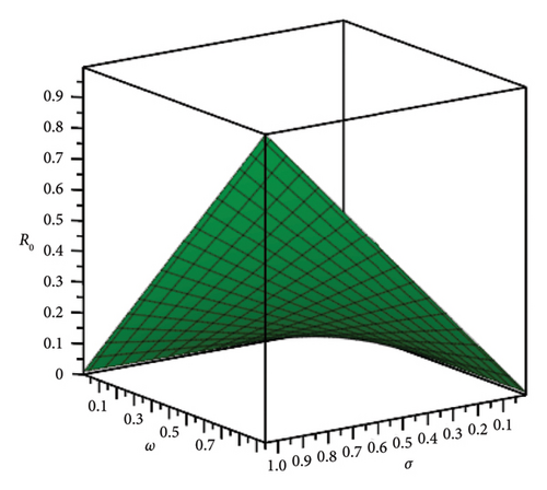
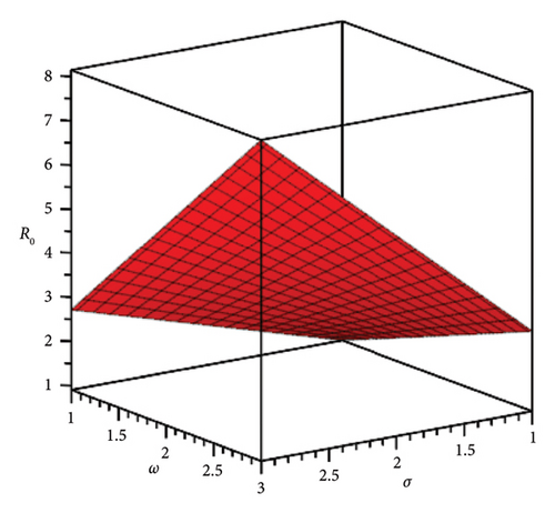
If R0 < 1, then E0 is locally stable, indicating a decrease in smoking behaviour within the population. If R0 > 1, then E0 is unstable, indicating that smoking behaviour will spread among the population. Figure 1 illustrates a graphical phase diagram of R0 in relation to σ and ω for system (8), where κ, η, and β are constant parameters from Table 1, highlighting the stable and unstable regions.
| Parameter | Description | Value (unit: 1/time) Source [15] |
|---|---|---|
| ω | Recruitment rate in P(t) | 1 |
| σ | Linkage index between S(t) and P(t) | 0.14 |
| κ | Natural mortality rate | 0.05 |
| β | Rate at which O(t) become S(t) | 0.002 |
| λ | Linkage index between Q(t) who might get back to smoking | 0.0025 |
| η | Smoking cessation rate | 0.8 |
| μ | Remaining fraction of smokers who permanently quit smoking | 0.1 |
3.4. Endemic Equilibrium
In this section, we assess the stability of the endemic equilibrium for the fractional smoking model. Using the system of equations provided in the model, we first compute the endemic equilibrium points and then analyse the stability using the Jacobian matrix and eigenvalues.
Using the parameter values from Table 1 and assuming S∗ = 1 for simplicity, we compute the approximate endemic equilibrium values as follows.
Given that all the real parts of the eigenvalues are negative, the endemic equilibrium E∗ is locally asymptotically stable for any fractional order 0 < α ≤ 1 [42].
4. Numerical Method
In this section, the Bernstein operational matrices approximation method [43] is presented using the Caputo fractional derivative properties and the collocation points to solve numerically the nonlinear system of fractional order of the epidemic smoking model presented in equation (8).
Consequently, solving the system of equation (43) can be done by finding the collocation points using the equation (45) and using the given initial conditions of (44) to calculate all the cj,i. Applying all this process will enable us to find approximate solutions g1(t), g2(t), …, gk(t) of the system of fractional order (26).
5. Numerical Results and Error Estimates
In this section, the application of the illustrated method in Section 4 on the given system of equations of fractional order for the smoking epidemic model presented in equation (8) with different parameters is demonstrated. Moreover, a comparison is made between the method in Section 4 with two recent methods applied to the same equation (8), i.e., q-HATM [15] and FDTM [16].
Specified values for the parameters in the system of equation (8) are given in Table 1 to verify the effectiveness and precision of the method used in this research.
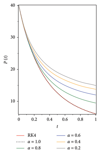
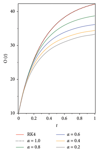
By finding the collocation points using equation (45) and using the given initial conditions in (48), we calculate all the cj,i with the help of Maple Software. Then, we find approximate solutions of P(t), O(t), S(t), Q(t) and L(t). The efficiency and accuracy of the presented method are verified when comparing it with the well-known Runge–Kutta fourth-order method (RK4).
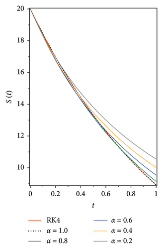
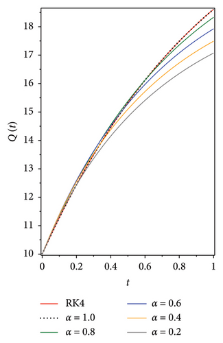
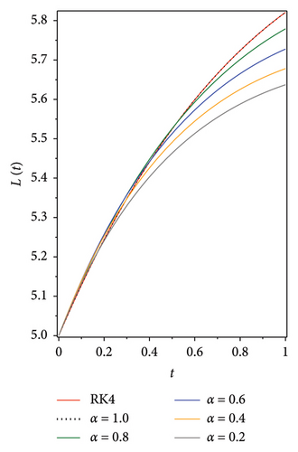
The following graphs show the approximate solutions of P(t), O(t), S(t), Q(t) and L(t) with different values of α, as shown in Figure 2. The accuracy and efficiency of the presented method are clearly seen in all the graphs. Moreover, Tables 2, 3, 4, 5 and 6 show the comparisons of the approximated solutions of the Bernstein operational matrices method with RK4, FDTM, and q-HATM for the given smoking epidemic model 8 at α = 1 and α = 0.9. The results show strong evidence for the validity of the presented method.
| P(t) | |||||||
|---|---|---|---|---|---|---|---|
| t | RK4 | α = 1 | α = 0.9 | ||||
| Present method | FDTM | q-HATM | Present method | FDTM | q-HATM | ||
| 0 | 40 | 40 | 40 | 40 | 40 | 40 | 40 |
| 0.1 | 30.5072 | 30.5063 | 30.9766 | 30.7667 | 30.3581 | 26.2807 | 29.1162 |
| 0.2 | 23.7850 | 23.7853 | 24.174 | 25.6668 | 23.8256 | 17.8878 | 26.0052 |
| 0.3 | 18.9262 | 18.9271 | 19.2495 | 24.7002 | 19.2628 | 12.8287 | 28.4733 |
| 0.4 | 15.3484 | 15.3480 | 15.6184 | 27.867 | 15.9889 | 9.6387 | 35.8752 |
| 0.5 | 12.6687 | 12.6675 | 12.8957 | 35.1672 | 13.5890 | 7.5495 | 47.8402 |
| 0.6 | 10.6306 | 10.6304 | 10.8229 | 46.6008 | 11.7965 | 6.1373 | 64.1152 |
| 0.7 | 9.0588 | 9.0596 | 9.223 | 62.1678 | 10.4314 | 5.158 | 84.5111 |
| 0.8 | 7.8313 | 7.8315 | 7.9727 | 81.8682 | 9.3728 | 4.4654 | 108.878 |
| 0.9 | 6.8620 | 6.8614 | 6.9847 | 105.702 | 8.5440 | 3.9687 | 137.095 |
| 1 | 6.0889 | 6.0890 | 6.1962 | 133.669 | 7.8904 | 3.6099 | 169.057 |
| O(t) | |||||||
|---|---|---|---|---|---|---|---|
| t | RK4 | α = 1 | α = 0.9 | ||||
| Present method | FDTM | q-HATM | Present method | FDTM | q-HATM | ||
| 0 | 10 | 10 | 10 | 10 | 10 | 10 | 10 |
| 0.05 | 15.0909 | 15.0913 | 14.5834 | 15.0559 | 15.2268 | 17.3313 | 16.6946 |
| 0.1 | 19.3402 | 19.3411 | 18.8789 | 19.0756 | 19.4832 | 23.474 | 20.6741 |
| 0.15 | 22.9048 | 22.9053 | 22.4858 | 22.059 | 22.9735 | 28.0928 | 22.8892 |
| 0.2 | 25.9090 | 25.9087 | 25.5286 | 24.0063 | 25.8561 | 31.6072 | 23.5858 |
| 0.25 | 28.4522 | 28.4513 | 28.1067 | 24.9173 | 28.2532 | 34.3096 | 22.8977 |
| 0.3 | 30.6140 | 30.6131 | 30.2999 | 24.7922 | 30.2590 | 36.4067 | 20.9135 |
| 0.35 | 32.4585 | 32.4582 | 32.1728 | 23.6308 | 31.9467 | 38.047 | 17.6978 |
| 0.4 | 34.0380 | 34.0385 | 33.7777 | 21.4332 | 33.3732 | 39.3381 | 13.3004 |
| 0.45 | 35.3950 | 35.3959 | 35.1575 | 18.1994 | 34.5835 | 40.3594 | 7.76208 |
| 0.5 | 36.5641 | 36.5653 | 36.3473 | 13.9294 | 35.6138 | 41.1701 | 1.11636 |
| S(t) | |||||||
|---|---|---|---|---|---|---|---|
| t | RK4 | α = 1 | α = 0.9 | ||||
| Present method | FDTM | q-HATM | Present method | FDTM | q-HATM | ||
| 0 | 20 | 20 | 20 | 20 | 20 | 20 | 20 |
| 0.1 | 18.4221 | 18.4221 | 18.5009 | 18.4244 | 18.3696 | 17.5281 | 17.9798 |
| 0.2 | 16.9756 | 16.9756 | 17.0509 | 16.9938 | 16.8930 | 15.2715 | 16.4515 |
| 0.3 | 15.6484 | 15.6484 | 15.7202 | 15.708 | 15.5537 | 13.3178 | 15.1913 |
| 0.4 | 14.4298 | 14.4298 | 14.4982 | 14.5671 | 14.3372 | 11.6235 | 14.1491 |
| 0.5 | 13.3102 | 13.3102 | 13.3753 | 13.5711 | 13.2309 | 10.1521 | 13.2994 |
| 0.6 | 12.2810 | 12.2810 | 12.3429 | 12.7201 | 12.2235 | 8.8727 | 12.626 |
| 0.7 | 11.3344 | 11.3344 | 11.3932 | 12.0138 | 11.3053 | 7.7594 | 12.1178 |
| 0.8 | 10.4633 | 10.4633 | 10.5192 | 11.4525 | 10.4675 | 6.7897 | 11.7662 |
| 0.9 | 9.6615 | 9.6615 | 9.7144 | 11.036 | 9.7023 | 5.9444 | 11.5645 |
| 1 | 8.9231 | 8.9231 | 8.9733 | 10.7645 | 9.0028 | 5.2073 | 11.5073 |
| Q(t) | |||||||
|---|---|---|---|---|---|---|---|
| t | RK4 | α = 1 | α = 0.9 | ||||
| Present method | FDTM | q-HATM | Present method | FDTM | q-HATM | ||
| 0 | 10 | 10 | 10 | 10 | 10 | 10 | 10 |
| 0.1 | 11.2780 | 11.2780 | 11.2142 | 11.276 | 11.3198 | 11.9966 | 11.6331 |
| 0.2 | 12.4398 | 12.4398 | 12.3791 | 12.4241 | 12.5034 | 13.7923 | 12.852 |
| 0.3 | 13.4959 | 13.4959 | 13.4382 | 13.4443 | 13.5654 | 15.3195 | 13.8408 |
| 0.4 | 14.4556 | 14.4556 | 14.401 | 14.3365 | 14.5184 | 16.6167 | 14.6413 |
| 0.5 | 15.3276 | 15.3276 | 15.2759 | 15.1008 | 15.3737 | 17.7164 | 15.2749 |
| 0.6 | 16.1194 | 16.1194 | 16.0705 | 15.7372 | 15.3737 | 18.6462 | 15.755 |
| 0.7 | 16.8381 | 16.8381 | 16.7919 | 16.2456 | 16.8297 | 19.4293 | 16.0913 |
| 0.8 | 17.4898 | 17.4898 | 17.4462 | 16.626 | 17.4471 | 20.0859 | 16.2908 |
| 0.9 | 18.0802 | 18.0802 | 18.0392 | 16.8786 | 18.0003 | 20.6329 | 16.3594 |
| 1 | 18.6145 | 18.6145 | 18.5759 | 17.0032 | 18.4954 | 21.0851 | 16.3015 |
| L(t) | |||||||
|---|---|---|---|---|---|---|---|
| t | RK4 | α = 1 | α = 0.9 | ||||
| Present method | FDTM | q-HATM | Present method | FDTM | q-HATM | ||
| 0 | 5 | 5 | 5 | 5 | 5 | 5 | 5 |
| 0.1 | 5.1283 | 5.1283 | 5.1218 | 5.128 | 5.1324 | 5.1998 | 5.1636 |
| 0.2 | 5.2438 | 5.2438 | 5.2377 | 5.2422 | 5.2499 | 5.3765 | 5.2841 |
| 0.3 | 5.3478 | 5.3478 | 5.342 | 5.3426 | 5.3540 | 5.5235 | 5.3803 |
| 0.4 | 5.4410 | 5.4410 | 5.4356 | 5.4291 | 5.4460 | 5.6446 | 5.4564 |
| 0.5 | 5.5245 | 5.5245 | 5.5194 | 5.5017 | 5.5271 | 5.7434 | 5.5148 |
| 0.6 | 5.5990 | 5.5990 | 5.5942 | 5.5605 | 5.5983 | 5.8229 | 5.5567 |
| 0.7 | 5.6653 | 5.6653 | 5.6608 | 5.6054 | 5.6606 | 5.8856 | 5.5832 |
| 0.8 | 5.7239 | 5.7239 | 5.7197 | 5.6365 | 5.7149 | 5.9338 | 5.595 |
| 0.9 | 5.7756 | 5.7756 | 5.7717 | 5.6537 | 5.7618 | 5.9693 | 5.5928 |
| 1 | 5.8209 | 5.8209 | 5.8173 | 5.657 | 5.8021 | 5.9939 | 5.577 |
Tables 7, 8, and 9 compare the absolute error of P(t), O(t), S(t), Q(t) and L(t) when α = 1 and n = 7 for Bernstein operational method, FDTM, q-HATM and RK4. The calculations show that the absolute error for all the functions in our presented method is less than the other two methods (FDTM and q-HATM).
| t | Absolute error of P(t) | Absolute error of S(t) | ||||
|---|---|---|---|---|---|---|
| Present method | FDTM | q-HATM | Present method | FDTM | q-HATM | |
| 0 | 0 | 0 | 0 | 0 | 0 | 0 |
| 0.1 | 9.0 × 10⁻⁴ | 4.7 × 10⁻¹ | 2.6 × 10⁻¹ | 3.3 × 10⁻⁷ | 7.9 × 10⁻² | 2.3 × 10⁻³ |
| 0.2 | 2.5 × 10⁻⁴ | 3.9 × 10⁻¹ | 1.9 × 100 | 2.4 × 10⁻⁷ | 7.5 × 10⁻² | 1.8 × 10⁻² |
| 0.3 | 8.9 × 10⁻⁴ | 3.2 × 10⁻¹ | 5.8 × 100 | 4.0 × 10⁻⁷ | 7.2 × 10⁻² | 6.0 × 10⁻² |
| 0.4 | 4.1 × 10⁻⁴ | 2.7 × 10⁻¹ | 1.2 × 101 | 2.4 × 10⁻⁷ | 6.8 × 10⁻² | 1.4 × 10⁻¹ |
| 0.5 | 1.1 × 10⁻³ | 2.3 × 10⁻¹ | 2.3 × 101 | 4.4 × 10⁻⁷ | 6.5 × 10⁻² | 2.6 × 10⁻¹ |
| 0.6 | 1.4 × 10⁻⁴ | 1.9 × 10⁻¹ | 3.6 × 101 | 2.0 × 10⁻⁷ | 6.2 × 10⁻² | 4.4 × 10⁻¹ |
| 0.7 | 8.4 × 10⁻⁴ | 1.6 × 10⁻¹ | 5.3 × 101 | 7.1 × 10⁻⁷ | 5.9 × 10⁻² | 6.8 × 10⁻² |
| 0.8 | 1.6 × 10⁻⁴ | 1.4 × 10⁻¹ | 7.4 × 10⁻¹ | 3.2 × 10⁻⁷ | 5.6 × 10⁻² | 9.9 × 10⁻¹ |
| 0.9 | 5.8 × 10⁻⁴ | 1.2 × 10⁻¹ | 9.9 × 101 | 1.2 × 10⁻⁷ | 5.3 × 10⁻² | 1.4 × 100 |
| 1 | 9.8 × 10⁻⁵ | 1.1 × 10⁻¹ | 1.3 × 10² | 8.4 × 10⁻⁷ | 5.0 × 10⁻² | 1.8 × 100 |
| t | Absolute error of Q(t) | Absolute error of L(t) | ||||
|---|---|---|---|---|---|---|
| Present method | FDTM | q-HATM | Present method | FDTM | q-HATM | |
| 0 | 0 | 0 | 0 | 0 | 0 | 0 |
| 0.1 | 1.1 × 10⁻⁷ | 6.4 × 10⁻² | 2.0 × 10⁻³ | 6.9 × 10⁻⁹ | 6.5 × 10⁻³ | 3 × 10⁻⁴ |
| 0.2 | 4.4 × 10⁻⁸ | 6.0 × 10⁻² | 1.6 × 10⁻² | 3.8 × 10⁻⁹ | 6.1 × 10⁻³ | 1.6 × 10⁻³ |
| 0.3 | 7.8 × 10⁻⁷ | 5.8 × 10⁻² | 5.2 × 10⁻² | 5.0 × 10⁻⁹ | 5.8 × 10⁻³ | 5.2 × 10⁻³ |
| 0.4 | 8.6 × 10⁻⁸ | 5.5 × 10⁻² | 1.2 × 10⁻¹ | 1.1 × 10⁻⁸ | 5.4 × 10⁻³ | 1.2 × 10⁻² |
| 0.5 | 1.8 × 10⁻⁷ | 5.2 × 10⁻² | 2.3 × 10⁻¹ | 2.5 × 10⁻⁸ | 5.1 × 10⁻³ | 2.3 × 10⁻² |
| 0.6 | 4.5 × 10⁻⁸ | 4.9 × 10⁻² | 3.8 × 10⁻² | 2.9 × 10⁻⁹ | 4.8 × 10⁻³ | 3.9 × 10⁻² |
| 0.7 | 1.2 × 10⁻⁷ | 4.6 × 10⁻² | 5.9 × 10⁻¹ | 6.9 × 10⁻⁸ | 4.5 × 10⁻³ | 6.0 × 10⁻² |
| 0.8 | 1.3 × 10⁻⁷ | 4.4 × 10⁻² | 8.6 × 10⁻¹ | 8.0 × 10⁻⁸ | 4.2 × 10⁻³ | 8.7 × 10⁻² |
| 0.9 | 2.7 × 10⁻⁷ | 4.1 × 10⁻² | 1.2 × 100 | 1.3 × 10⁻⁷ | 3.9 × 10⁻³ | 1.2 × 10⁻¹ |
| 1 | 8.5 × 10⁻⁷ | 3.9 × 10⁻² | 1.6 × 100 | 1.6 × 10⁻⁷ | 3.6 × 10⁻³ | 1.6 × 10⁻¹ |
| Absolute error of O(t) | |||
|---|---|---|---|
| t | Present method | FDTM | q-HATM |
| 0 | 0 | 0 | 0 |
| 0.05 | 4.0 × 10⁻⁴ | 5.1 × 10⁻¹ | 3.5 × 10⁻² |
| 0.1 | 9.2 × 10⁻⁴ | 4.6 × 10⁻¹ | 2.6 × 10⁻¹ |
| 0.15 | 5.4 × 10⁻⁴ | 4.2 × 10⁻¹ | 8.5 × 10⁻¹ |
| 0.2 | 8.9 × 10⁻⁴ | 3.8 × 10⁻¹ | 1.9 × 100 |
| 0.25 | 8.9 × 10⁻⁴ | 3.5 × 10⁻¹ | 3.5 × 100 |
| 0.3 | 4.0 × 10⁻⁴ | 3.1 × 10⁻¹ | 5.8 × 100 |
| 0.35 | 3.5 × 10⁻⁴ | 2.9 × 10⁻¹ | 8.8 × 100 |
| 0.4 | 4.1 × 10⁻⁴ | 2.6 × 10⁻¹ | 1.3 × 101 |
| 0.45 | 9.9 × 10⁻⁴ | 2.4 × 10⁻¹ | 1.7 × 101 |
| 0.5 | 1.1 × 10⁻³ | 2.2 × 10⁻¹ | 2.3 × 101 |
6. Residual Correction Technique
In this section, we introduce a residual correction technique to approximate the solutions for the system of differential equations by minimising the absolute error to the greatest extent possible.
Let gj(t) and be the exact and the approximate solutions, respectively, of equation (26). In the following technique, a residual correction can be applied to improve the estimations of the absolute error.
We solve equation (51) using the presented method in Section 4 with degree m such that m > n, where having the following initial condition .
Corollary 1. Let and be the approximate solutions of equations (26) and (51), respectively. Then, is considered the corrected approximate solution of equation (26) having the following error function . Taking into consideration that if , then is the estimation of the absolute error. Furthermore, if , we can conclude that is more precise solution compared with in any given norm. The optimal n in the presented method that finds the minimal absolute error might be found by at any given norm.
Corollary 2. To find the approximate solutions for different values on n, we start first by using the triangle inequality that implies the following.
If K > 1, then both absolute errors can be considered very good approximations.
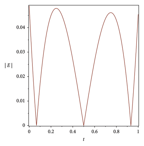
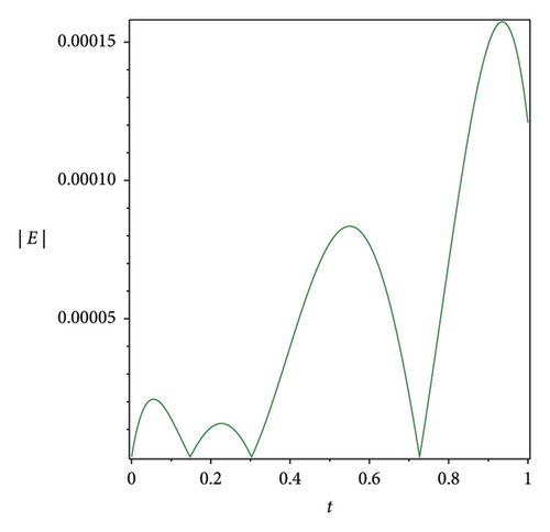
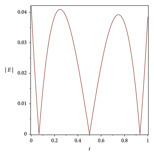
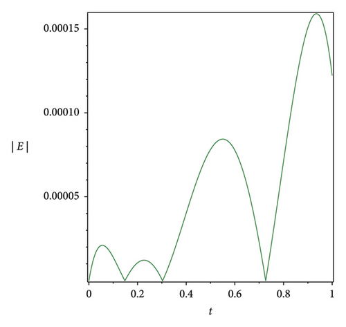
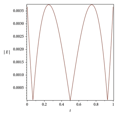
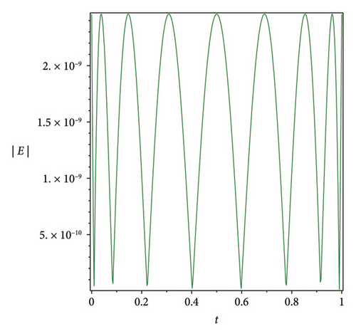
The efficiency residual correction technique is shown in Figure 3 where the absolute error function at n = 3 is much higher compared with the corrected absolute error function at n = 3 and m = 8 of the Bernstein operational matrices method at α = 1 for S(t), Q(t) and L(t), which shows the applicability, efficiency and accuracy of the corrected absolute error technique.
7. Discussion
The numerical results reveal distinct behaviours among the subgroups P(t), O(t), S(t), Q(t) and L(t) as the fractional order α varies, providing meaningful insights into smoking behaviour modelling. For α = 1, where memory effects are minimal, the decline in potential smokers P(t) and smokers S(t) is rapid, while permanent quitters L(t) increase quickly, indicating that interventions yield faster results. In this case, occasional smokers O(t) and temporary quitters Q(t) stabilise quickly, reflecting faster relapse and cessation dynamics. As α decreases (i.e., α < 1), the model incorporates stronger memory effects, leading to slower declines in P(t) and S(t) with more gradual transitions between states. This suggests that smoking behaviour becomes more persistent and deeply rooted, making cessation efforts more challenging. Prolonged fluctuations in O(t) and Q(t) further highlight the potential for relapse over time, underscoring the importance of sustained public health interventions. The reproduction number R0 plays a crucial role in determining the system’s stability, with R0 < 1 predicting a decline in smoking prevalence and R0 > 1 indicating sustained or growing smoking behaviour. This implies that policies must aim to maintain R0 < 1 by promoting smoking cessation and reducing initiation rates. In addition, the comparison between the Bernstein operational matrices method and other approaches—such as Runge–Kutta, FDTM and q-HATM—demonstrates the Bernstein method’s superior accuracy, efficiency and reduced computational error. These results validate the utility of Bernstein polynomials in solving complex nonlinear fractional models, reinforcing their value for studying public health dynamics.
8. Conclusions
This paper utilised the Bernstein operational matrices method to numerically solve a nonlinear system of fractional differential equations. By applying this method to the smoking epidemic model, we demonstrated its effectiveness and significance in this context. Our results underscored the method’s efficiency when compared with traditional approaches such as Runge–Kutta, emphasising the importance of integrating advanced techniques such as the Bernstein operational matrices method in modelling real-world problems. Furthermore, our findings revealed superior approximation outcomes compared with FDTM and q-HATM. In addition, the residual corrected error technique introduced in this research efficaciously minimised absolute error functions by refining previous approximation solutions for the given smoking model. The reliability of the model’s long-term predictions, derived from almost a decade of numerical analysis, is generally strong, particularly in capturing key trends in smoking behaviour over time. However, several factors could significantly alter these predictions, such as changes in public health policies, technological advances in cessation methods, the introduction of new tobacco products like e-cigarettes or shifts in societal attitudes towards smoking. These potential influences highlight the importance of continuously updating the model to maintain its accuracy and relevance. The presented method effectively captures the memory effect in smoking dynamics; however, future research could address constraints such as external influences affecting smoking behaviour and use sensitivity analysis to understand how parameter changes impact results. The application of machine learning for parameter estimation could further enhance model accuracy by adapting to real-time data. In addition, studying the social and economic aspects that influence smoking would improve the mathematical model and its use in public health planning. Finally, the successful implementation of the presented method in addressing epidemic models generates new research opportunities for precise simulation and analysis of complex systems across many disciplines of study.
Conflicts of Interest
The authors declare no conflicts of interest.
Funding
The research was supported entirely by personal funds.
Open Research
Data Availability Statement
The datasets generated and analysed during the current study are available from the corresponding authors upon reasonable request.


