Incorporating distributed generation (DG) technology into modern power systems heralds a multitude of technological, economic, and environmental advantages. These encompass enhanced reliability, reduction in power losses, heightened efficiency, low initial investment requirements, abundant availability, and a minimized environmental footprint. However, the rapid detection and disconnection of DG units during islanding events are paramount to circumvent safety hazards and potential equipment damage. Although passive techniques are predominantly utilized for islanding protection due to their minimal systemic interference, their susceptibility to substantial nondetection zones (NDZ) instigates a transition toward more innovative techniques. Addressing this crucial need, the study employs a novel amalgamation of signal processing methodologies and a suite of intelligent classifiers to augment the detection of islanding events in power systems. Concealed features from a variety of signals are extracted by the methodology and utilized as robust inputs to the intelligent classifiers. This empowers these classifiers to make a reliable distinction between islanding events and other types of disturbances. The breadth of the study is expanded to evaluate a range of sophisticated models including gradient boosting, decision tree–based models, and multilayer perceptrons (MLPs). These models are thoroughly tested on a radial distribution system integrated with two DG units and subjected to rigorous simulations and comparative analysis using the DIgSILENT Power Factory software. The findings underscore the efficacy of the proposed method, showcasing a significant improvement over conventional techniques in terms of efficiency and resilience. Above all, the methodology exhibits an exceptional ability to discriminate between islanding events and other system disturbances. Specifically, the islanding detection method demonstrated a detection time of less than one cycle (20 ms), ensuring rapid response. Moreover, the proposed algorithm demonstrated the capability to detect all ranges of power mismatch, including zero-power mismatch, thereby eliminating the NDZ. These results illuminate the benefits of integrating signal processing methodologies with intelligent classifiers, marking a significant stride forward in the realm of islanding event detection.

1. Introduction

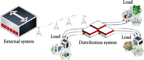
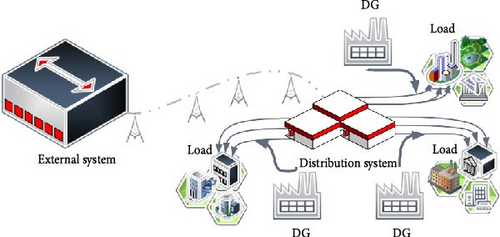
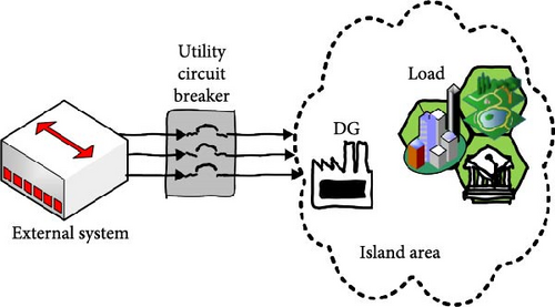
To fulfill the requirements of electrical load demands, distributed energy resources assume a significant role in the distribution systems. In contemporary times, there has been a surge in the utilization of renewable energy resources in the distribution system. This trend is attributed to the need to meet the escalating demand for electricity and address the global predicament associated with conventional energy sources such as coal, oil, and natural gas. Within the power system, the integration of distributed generation (DG) units into the utility infrastructure brings about several beneficial alterations, such as reducing air pollution, improving reliability and better power quality, and decreasing of the power losses. Figures 1 and 2 in this study demonstrate a notable contrast between conventional distribution systems and those with multiple embedded configurations, wherein supplementary DG units are often installed in close proximity to the local load. The conventional techniques employed in energy generation and dissemination are undergoing a transformation, thereby presenting novel challenges in the preservation of grid stability. In addition to these favorable effects, various technical challenges emerge, including concerns related to islanding detection, false tripping, system safety, and system stability and reliability. The depiction in Figure 3 highlights a crucial challenge associated with the integrations, namely, the islanding event that can be intentionally or unintentionally. The problematic scenario arises in the form of unintentional islanding, which occurs due to external factors and actions beyond the control of the DG plant controller [1]. If the system operates in island mode, it is imperative for the active segment of the distribution system to promptly detect the disconnection from the primary grid. Swiftly removing fast DG is considered a vital necessity in accordance with globally enforced DG connection codes. This precautionary measure is implemented to prevent equipment malfunctions, address grid safety concerns, and mitigate potential hazards to personnel safety [2]. Consequently, in the event of an islanding occurrence, it becomes imperative to swiftly disconnect all DGs sources that find themselves in an islanded state. Therefore, the islanding detection methods are studied by researchers and typically categorized into two primary groups as illustrated in Figure 4, each serving as a fundamental strategy for effectively detecting such events within power systems. The first approach involves the remote technique, wherein measurements and monitoring are executed on the utility side of the system. In contrast, the second method employs the local technique, entailing measurements and monitoring on the DG side of the power system. These techniques collectively play a pivotal role in ensuring the rapid and accurate identification of islanding events, contributing to the overall stability and safety of power systems. Several essential aspects can be used to assess how well islanding detection approaches work. The nondetection zone (NDZ) is the most prevalent feature, while the Q factor determines the sensitivity of the detection algorithm. Due to the disparity in power supply and load, NDZ is regarded as the region where islanding cannot be identified. The islanding detection approach fails to detect the islanding during the required time interval if the mismatch of active and reactive power between the DG generating power and load consuming power is too small [3]. Mathematically, the NDZ is expressed as NDZ = k·Q, where k is a constant that depends on the specific characteristics of the algorithm and the system under consideration [3]. The present study endeavors to develop a straightforward methodology that can effectively evaluate the state of islanding by discriminating between systemic islanding and nonislanding conditions.

Details are in the caption following the image — **Figure 1**
Open in figure viewer PowerPoint

Conventional distribution systems.

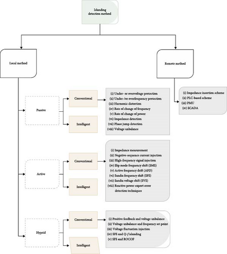
The proposed techniques encompass a diverse range of approaches; remote approaches rely on communication between DGs and utility circuit breakers via a central control unit and monitoring system. The central control unit obtains status signals from the circuit breakers through a communication channel that encompasses different channels such as fiber optic, private or leased digital networks, analog phone lines, digital phone lines, power line carriers, wireless radio, and two-wire transmission lines. Subsequently, the primary controller assesses the condition of the isolated power system and transmits the alert to the requisite distributed generators that constitute the island. These systems are considered resilient for islanding detection due to the absence of NDZ concerns. In [4], some remote approaches which briefly discussed the implementation of these strategies necessitate substantial financial investment, particularly at the infrastructural level. The main drawbacks of these remote techniques stem from their costly implementation, which is further compounded when employed in networks of limited scale. The local islanding detection approach pertains to the microgrid (MG) side. These methods are categorized into active, passive, or hybrid techniques which used to determine whether the grid voltage and frequency exceed the limits set by the applicable standard. Consequently, certain researchers are directing their focus toward the creation and execution of an islanding detection algorithm that employs a local approach. This approach necessitates the acquisition of measurements at the DG site, without the need for any communication infrastructure. The local method collects signal information, including voltage, frequency, harmonic distortion, and current, at the point of common coupling (PCC) between the DG site and the utility grid. In the island mode, the previous parameters exhibit significant variation contingent upon the power mismatch that exists between the system and the DG. According to recent research works, the passive islanding detection method is preferable even in cases in which the negative contribution of the active techniques can be considered negligible. The threshold values assigned to each of these variables distinguish islanding and grid-connected modes. The authors proposed an islanding detection method in reference [5], which utilizes voltage unbalance and total harmonic distortion of the current as two conventional variables. This approach enables the detection of islanding events without altering the DG loading variation. The study conducted by Zeineldin, El-Saadany, and Salama [6] delves into the impact of DG interface control on islanding detection and the assessment of the NDZ concerning overvoltage and undervoltage protection and overfrequency and underfrequency protection. This investigation employs a range of interface control techniques, such as constant current, constant active power–voltage (P-V), and constant active power–reactive power (P-Q) controls, to comprehensively evaluate their effects and outcomes. Conversely, in [7], the researchers conducted an investigation that involved a comparative and analytical examination of three passive anti-islanding techniques: undervoltage, under-/overfrequency, and the positive sequence impedance method. Among these approaches, the positive sequence impedance method demonstrated the swiftest response in detecting islanding events, as established by their findings.

In the context of islanding detection, the theories of instantaneous power and advanced power found application. As illustrated in [8], the technique under examination relied on the computation of instantaneous power at the PCC. This particular method exhibited notable success in the identification of islanding events within a constrained set of sampling intervals, as detailed in the referenced study. A technique was proposed in [9] that utilizes the instantaneous active and reactive power at the PCC of a MG. The MG in question comprises a natural gas–fired generator, a doubly-fed induction generator-type wind generator, a solar generator, and associated local loads. The power systems computer aided design (PSCAD)/electromagnetic transients including DC (EMTDC) simulator was utilized to evaluate the efficacy of the proposed technique in diverse scenarios, such as islanding conditions for multiple outputs of the MG and fault conditions that altered the fault’s position, type, inception angle, and resistance. The authors of [10] proposed a methodology that integrates the synchronous reference frame technique with conservative power theory. This approach has been employed to extract pertinent characteristics from three-phase electrical voltage signals under faulty conditions. The ultimate goal of this methodology is to detect and recognize islanding events. However, the major drawback of passive methods is the difficulty in distinguishing when load and generation are almost equal in an islanded distribution system. This situation may result in extensive NDZ. There have been numerous studies suggesting that traditional methods of islanding detection are being replaced by machine learning combined with signal processing methods. The integration of intelligent classifiers and signal processing techniques suggests the feasibility of achieving the objective of islanding detection. The prevalent intelligent classifiers utilized in islanding detection techniques based on signal processing include various decision trees (DT), adaptive neuro-fuzzy inference systems (ANFIS), random forests (RF), support vector machines (SVM), and fuzzy logic control. As a result, these methods are a sensible choice for islanding detection because of their ability to pick appropriate thresholds for detection as well as their ability to deal with complex conditions. Off-grid functioning may be estimated as fast as possible without any communication with utility components or concessions on power quality, which is the primary goal of these techniques. In addition to providing rapid estimation, the method offers excellent computational efficiency and good dependability and precision. For instance, in [11], the authors suggested an artificial neural network (ANN)-based technique for distributed synchronous generator islanding detection. In the study conducted by Kumar et al. [12], the investigation centered on the detection of islanding events in photovoltaic-based distributed power generation (PV-DPG). This approach hinged on the utilization of a variable Q-factor wavelet transform in combination with an ANN. Impressively, this methodology achieved an accuracy rate of 98% in categorizing PV-DPG states as either in an islanded condition or not, facilitated by the ANN classifier. Furthermore, the results underscored the robustness of this approach, demonstrating its effectiveness in environments characterized by varying levels of noise. Simultaneously, numerous other techniques, such as the Gray Wolf optimized artificial neural network (GWO-ANN), the probabilistic neural network (PNN), the extended neural network (ENN), the backpropagation neural network (BPNN), the self-organizing map (SOM), and the modular probabilistic neural network (MPNN), have been explored for islanding detection. In a parallel endeavor, authors in [13] introduced an intelligent islanding algorithm founded on multivariate analysis and data mining techniques. This innovative method generates DT that specify the thresholds, protection strategies, and tripping logic for each DG islanding relay deployed within the distribution network. The intelligent islanding relay (IIR) crafted using this approach consistently outperforms currently deployed islanding devices, offering higher levels of reliability and security while exhibiting a notably reduced NDZ. Additionally, a scholarly article cited as [14] proposed a method for detecting islanding events in hybrid systems, adding to the repertoire of islanding detection strategies.

The primary innovation of this approach was the utilization of a DT and Sandia Frequency Shift (SFS) for DG systems that are connected to the grid via inverters. The efficacy of the proposed approach was validated through a comprehensive analysis of case studies involving power imbalances, power quality incidents, and the presence of one or more inverter-based DG units connected to the grid. This research developed a strategy that consists of two primary stages to overcome the limitations of existing islanding detection methods. The first phase is to extract features from the target DG location using GT, a more general form of the short-time Fourier transforms (STFT) which explicitly defines direct (analysis) and inverse (synthesis) equations [15]. GT is a mathematical method used for signal analysis such as photos, audio, and voices. It is a sort of time–frequency analysis in which a signal is decomposed into its constituent frequencies across time. Many more features than with other tools can be extracted using this processing method. In the refined methodology, a classification task is executed under islanding conditions employing a diverse set of machine learning algorithms, which consist of gradient boosting models (CatBoost, eXtreme Gradient Boosting [XGBoost], and LightGBM), DT-based models (DT, RF, and extremely randomized trees [ExtraTrees]), and several architectures of multilayer perceptron (MLP) ANN. These algorithms are designed to learn from the complex patterns within the data and provide an insightful understanding of the occurrence of islanding events in contrast to other system disturbances. Each of these models undergoes an extensive performance evaluation, and their outcomes are juxtaposed to determine their respective efficacies. The exploration of error measurement indices guides in identifying the optimal features and classification techniques to detect islanding with precision. Considering the prevailing challenges with the existing algorithms for islanding detection, this manuscript is suggested, and it relies on the research conducted by the authors in their master research, “An Intelligent Passive Islanding Detection and Classification Scheme for A Radial Distribution System” [16]. The newly devised technique employs Gabor feature extraction in conjunction with the CatBoost algorithm, a novel application in the field of islanding detection. Validation of this methodology is conducted through simulations, followed by a comparative analysis with existing techniques. Additionally, the thesis delivers a comprehensive examination of various islanding detection approaches, offering insights into their respective strengths and limitations. In this manuscript, the utilization of intelligent classifiers is extended, and a comparative analysis of their performance is discussed. Therefore, this work is showcasing notable advancements like the following:

•
An innovative islanding detection method leveraging the Gabor transform (GT) in combination with an assortment of classifiers to differentiate between islanding and nonislanding events in power systems is proposed.
•
The GT serves as a feature extraction tool, unraveling concealed characteristics from the instantaneous power for each phase and voltage signals at the target DG, which are then fed into the classifiers.
•
The suite of classifiers, including the CatBoost intelligent classifier and others, is proposed to enhance the accuracy of the classification of islanding events.

The structure of the paper is as follows: Section 2 describes the tools and methods used for the proposed islanding detection method. Section 3 provides the procedure for the islanding detection employing the proposed algorithm, while Section 4 provides a description of the studied system. Finally, Section 5 provides the simulation results used to assess the algorithm’s performance.

2. Proposed Islanding Detection Algorithm

The challenge of detecting islanding is addressed as a multiclass classification problem in this study. Thus, this section elucidates the tools and methodologies employed for the proposed islanding detection algorithm. The suggested algorithm encompasses the computation of instantaneous power for each phase, the implementation of the GT technique, and the deployment of a selection of classifiers. Initially, the core principle of instantaneous power theory is explicated. Subsequently, the theory of the GT technique is detailed. Finally, a thorough discussion on the set of classifiers, including but not limited to the CatBoost classifier, is provided. These classifiers encompass gradient boosting models (CatBoost, XGBoost, and LightGBM), DT-based models (DT, RF, and ExtraTrees), and several architectures of MLP ANN, each contributing to the identification and classification of islanding events.

2.1. Instantaneous Power Theory

In power systems, the relationship between active power (P) and system frequency (f) and reactive power (Q) and system voltage (V) is crucial. Variations in active power directly affect system frequency; an increase in active power demand lowers frequency, while a decrease in demand raises it. On the other hand, reactive power significantly impacts voltage levels. An increase in reactive power demand causes a voltage drop, whereas an excess of reactive power results in a voltage rise. Thus, frequency regulation is vital for balancing active power, and voltage control is essential for managing reactive power, both contributing to overall system stability and efficiency. Within this framework, the theory of instantaneous power is pivotal for understanding and characterizing the dynamic behavior of power systems. Instantaneous power, denoted as p(t), is a fundamental concept that quantifies the rate at which electrical energy is transferred or consumed at any given moment in time. Instantaneous power can be mathematically expressed as the product of voltage (V(t)) and current (I(t)) at a specific instant in time; that is, p(t) = V(t) × I(t). This formulation reflects the instantaneous interaction between voltage and current, representing the real power component. In alternating current (AC) systems, where both voltage and current are time-varying sinusoidal waveforms, instantaneous power provides insights into how electrical energy is being transmitted and utilized over time. To further refine the analysis and control of power systems, two key methodologies, namely, p-q theory and d-q theory, were used. p-q theory is also known as instantaneous power theory. p-q theory is primarily used for analyzing and controlling three-phase power systems. It decomposes instantaneous power into active and reactive components, facilitating real-time power quality improvement, harmonic compensation, and active filtering. In contrast, d-q theory, or direct-quadrature theory, is mainly utilized in the control of rotating machines and AC motor drives. It transforms three-phase time domain signals into two orthogonal components in a rotating reference frame, simplifying the analysis and control of AC machines by converting AC quantities into direct current (DC) quantities. In this paper, the use of p-q is crucial; one prominent aspect of p-q theory is the abc to αβ0 transformation, which provides a means of quantifying and separating active (P_3ϕ) and reactive power (Q_3ϕ) components in electrical systems, enabling precise measurement and control. P_3ϕ provides comprehensive insights into the power demands and energy flow of all three phases (a, b, and c), ensuring an accurate representation of power utilization in complex industrial, commercial, and distribution settings. It is computed as the sum of the instantaneous product of phase voltages and currents for each phase. This instantaneous power calculation further enhances the capabilities of the p-q theory, providing valuable insights into the operation of three-phase systems [17]:

(1)

It is determined through the computation of the instantaneous product of phase voltages denoted as v_a, v_b, and v_c. Meanwhile, the respective phase currents are denoted as i_a, i_b, and i_c at any given moment in time. The terms (v_ai_a, v_bi_b, v_ci_c) describe the instantaneous active power for each phase separately which is defined as follows:

(2)

The expression pertains to the phase number denoted by k, the maximum voltage value represented by V_m, the maximum current value represented by I_m, and the angular frequency represented by ω in units of rad/second. As evidenced by Equation (2), the instantaneous power per phase can be expressed as the sum of two distinct components: a constant term, denoted as (V_mI_m)/2, and a fluctuating term, represented by, . The proposed method utilizes instantaneous active power per phase.

2.2. GT

The GT is a time–frequency analysis technique that extends the capabilities of the STFT. The STFT is a widely used method for analyzing nonstationary signals, and the GT is one of several approaches in this field that works by analyzing signals in both the time and frequency domains, making it suitable for capturing complex variations in data. It decomposes signals into time–frequency components using a set of Gaussian functions called Gabor kernels. These kernels are applied to the signal, producing a representation that highlights both local frequency content and temporal behavior. By extracting features from this transformed data, such as spectral energy distribution or dominant frequency components, the GT approach enables detailed analysis and characterization of various phenomena. Overall, GT provides a powerful tool for signal analysis, particularly in applications where both time and frequency information are critical. The study referenced in [18] employed the use of GT as a proficient methodology for the categorization and recognition of power quality anomalies. The fundamental divergence between the STFT and the conventional FT resides in their approach to the window function w(s). Through the systematic shifting of the window function along the temporal axis and its application to the spectrogram generated by the Fourier transform, the STFT method is adept at scrutinizing the intricate time–frequency attributes inherent to the signal. Formally, the STFT can be rigorously defined as follows:

(3)

The equation involves a sliding variable of time denoted as t, an angular frequency represented by ω, a signal function in the time domain denoted as τ, and a window function denoted as w (τ). The GT can be considered as a derivative of the STFT, wherein the customary window function is replaced with a Gaussian function, a distinction visually depicted in [19]:

(4)

The Gaussian function g(τ) of a particular length can be derived in the following manner:

(5)

The final description employed for GT is the subsequent:

(6)

The window length is determined by the coefficient α. Consequently, it exerts a direct impact on the resolution of time and frequency [20]. It is evident from the final definition that the GT constitutes a unique manifestation of the STFT framework, characterized by the adoption of the Gaussian function as its window function. As elucidated in [15], the incorporation of the Gaussian window in the GT configuration affords optimal time–frequency resolution by efficiently concentrating energy within the time–frequency domain. An analogous technique, the discrete GT (DGT), presents another variant of the STFT, employing the Gaussian window function. The expansion of a finite and periodic sequence x[i] can be expressed as a linear combination of the Gabor coefficients (GC) and basis functions h_m,n[i]:

(7)

The discrete GC, represented as C_m,n, are derived in the following manner:

(8)

The dual basis of h[i] is represented by γ[i], and together, they constitute a biorthogonal basis. Ultimately, the DGT is formally characterized in the following manner:

(9)

where

, and ∆M and ∆N represent time and frequency sampling intervals, respectively. M and N represent the quantities of sampling in the temporal and spectral domains, respectively. The variable L denotes the number of samples, specifically referring to a window of L points as described in [21]. A set of comprehensive disturbances is formed through the utilization of simulations that rely on detection algorithms. The present study employed the technique of GT to extract distinct characteristics from voltage and instantaneous power signals per phase, with the aim of detecting instances of islanding and nonislanding.

2.3. Implementation of Diverse Machine Learning Algorithms

2.3.1. Gradient Boosting Techniques

Gradient boosting, a potent machine learning technique, constructs an ensemble of weak learners, often in the form of DT, in a step-by-step, stage-wise manner. It utilizes the idea of boosting, where simple models, known as weak learners, are combined to create a single powerful model, known as a strong learner. The model for gradient boosting is defined as follows:

(10)

Here, f_i (x) represents the output of the ith DT for the data point x. The aim of gradient boosting is to reduce the difference between the actual target values (y) and the model predictions (F (x)), as defined by a certain loss function L (y, F (x)).

During each iteration, a new tree is fitted to the negative gradient of the loss function with respect to the predictions of the current ensemble. This has the effect of moving the model’s predictions along the gradient descent direction in the output space [22].

2.3.1.1. CatBoost Algorithm

The term “CatBoost” is a portmanteau of “categorical” and “boosting.” It is a machine learning technique that is based on the concept of gradient boosting, which has broad applications in various domains such as fraud detection, recommendation systems, and forecasting. CatBoost is a novel open-source machine learning algorithm that has been designed to effectively handle categorical features characterized by a discrete set of values, commonly referred to as categories, which are not necessarily comparable. As a result, these features cannot be directly utilized in binary DT [23].

The mathematical definition of a category involves the utilization of an input vector, while network classifiers are trained through the use of data that possesses a general classification. Several machine learning techniques employ rudimentary approaches like one-hot encoding. In a similar vein, CatBoost conducts one-hot encoding automatically to convert categorical data into numerical data. Another approach is target encoding (TE) by replacing the categorical value with the mean target value of the training data for that value of the categorical variable [24]. CatBoost also has the option to utilize ordinal encoding (OE) if the categorical feature has an ordinal nature [25]. This can be done by passing a list of the categorical feature names to the cat_features parameter when creating the model and then selecting one of the aforementioned methods according to the categorical feature type. In contrast to deep learning, CatBoost does not necessitate vast datasets for extensive training. CatBoost is a machine learning algorithm that involves various hyperparameters such as regularization, learning rate, number of trees, tree depth, and others. However, it is noteworthy that CatBoost does not necessitate exhaustive hyperparameter tuning. This characteristic of CatBoost proves advantageous by mitigating the risk of overfitting. CatBoost adopts a distinctive algorithm for managing categorical features, comprising a three-step procedure for converting such features, if they exceed a designated threshold for category count, into numerical features [26].

The input observations undergo multiple random permutations.

The categorical or floating point label values undergo a transformation process to be represented as integer values.

The conversion of categorical features into numerical features follows a specific formula, as articulated in the ensuing equation as follows:

(11)

The variable InClassCounter denotes the frequency of instances where the class label is equal to 1, across all records that possess the present feature value. The initial value for the numerator, known as the prior, is established during parameter initialization. The variable TotalCounter denotes the cumulative count of observations with identical categorical values as the present observation, encompassing all records up to the immediately preceding one [27]. Consider a dataset denoted by H = {({X_j, y_j)} j = 1,2,.,.,.m, where

represents a vector comprising n features and the response feature y_j ∈ R, which can be binary (i.e., yes or no) or encoded as a numerical feature (0 or 1). The set of samples denoted as (X_j, y_j) exhibits an independent and identical distribution by an unspecified distribution P (.,.). The objective of the learning task is to effectively train a function H, which maps from the n-dimensional Euclidean space to the real numbers, such that it optimally addresses the given problem of regression, classification, or multiclassification for any input object. Function H is expected to minimize the anticipated loss, as specified as follows:

(12)

The aforementioned equation involves a smooth loss function denoted by L (,) and a testing dataset (X, y) that has been sampled from the training data H. The gradient boosting methodology involves the iterative construction of a sequence of approximations denoted as

; t = 0, 1,… in a greedy manner. The values of H^t, H^t−1 are derived through an additive procedure, where H^t = H^t−1 + αg^t. Here, α represents the step size, and g^t is a base predictor function that maps from

to R. The function g^t is selected from a set of functions G, with the aim of minimizing the expected loss as defined as follows:

(13)

Frequently, the task of minimizing is tackled through the utilization of the Newton method, which involves employing a second-order approximation of

(H^t−1 + g) at H^t−1, or alternatively, by implementing a (negative) gradient step. Both of these functions correspond to the gradient descent algorithm as described in [28]. Ordered boosting is a technique in which the training data points are arranged in a predetermined order (σ). Instead of producing a single model, CatBoost generates multiple models by gradually increasing the number of training instances in each model in the specified order (σ). The following is the presentation of the ordered boosting procedure:

i.
The initial step involves gathering data from either simulations or measurements for both the input and target (D).
ii.
The second step involves the assembly and preprocessing of the training data, denoted as t.
iii.
The third step involves the identification of (σ) by utilizing random permutations of t.
iv.
Proceed to compute the residuals (r) as the difference between the observed values and the predicted values.
v.
In the fifth step, the models are updated by incorporating the corresponding calculated residuals.

2.3.1.2. LightGBM

LightGBM is a gradient boosting framework that uses a tree-based learning algorithm. It differs from other tree-based algorithms by using a leaf-wise tree growth strategy, where the tree grows by splitting the leaf that reduces the loss the most rather than growing level-wise. This strategy can result in better performance and less memory usage. LightGBM also handles categorical features by using exclusive feature bundling (EFB) to reduce the dimensionality of the feature space. Moreover, LightGBM introduces two novel techniques: gradient-based one-side sampling (GOSS) and EFB. GOSS keeps all the instances with large gradients and performs random sampling on the instances with small gradients. EFB bundles mutually exclusive features (categorical variables) together to reduce the number of features, hence making the algorithm more efficient [29].

2.3.1.3. XGBoost

XGBoost is another gradient boosting algorithm known for its execution speed and model performance. It also uses a novel split-finding algorithm to handle sparse data and missing values directly. XGBoost has a regularization term in the objective function, which controls the model’s complexity and prevents overfitting. This regularization makes XGBoost a regularized version of gradient boosting, hence improving its performance on many datasets [30].

In summary, LightGBM uses a histogram-based algorithm for fast and efficient training, handling high-dimensional and sparse datasets effectively. XGBoost is a versatile gradient boosting framework with flexible hyperparameter tuning, suitable for general purpose tasks. CatBoost excels in handling categorical data natively and provides fast training, particularly for datasets with categorical features. Table 1 shows the differences between comparison between gradient boosting-based models.

Table 1. Main feature comparison between gradient boosting-based models.

Feature	LightGBM	XGBoost	CatBoost
Main idea	Histogram-based algorithm	Gradient boosting framework	Handling categorical data
Categorical data handling	Converts to numeric/one-hot	One-hot/label encoding	Native support
Speed	Fast	Moderate	Fast with categorical data
Memory usage	Efficient	Higher	Efficient
Tree growth strategy	Leaf-wise	Depth-wise	Symmetric
Interpretability	Feature importance, SHAP	Feature importance, SHAP	Feature importance, SHAP
Hyperparameter tuning	Flexible, many parameters	Flexible, many parameters	More straightforward
Use cases	High-dimensional, sparse	General purpose	Categorical features

Note: All gradient boosting based models utilize shapley additive explanations (SHAP) for input-output interpretation.

2.3.2. DT

2.3.2.1. General DT Models

DT algorithms represent a significant tool in the machine learning domain. They function by splitting data into subsets based on attribute values, creating a DT with branches representing the possible outcomes. This process starts at the tree’s root and advances toward the leaf nodes, representing the decision or classification. Information gain or Gini impurity measures typically guide the splitting criterion in DT algorithms.

A DT’s split point optimization utilizes the Gini impurity or information gain as follows:

(14)

where p(j | t) is the relative frequency of class j at node t:

(15)

where S is the set of all examples, Sv is the subset of examples in S for which attribute A has value v, and Entropy(S) is as follows for all classes I:

(16)

2.3.2.2. RF

RF is an ensemble learning method that operates by constructing multiple DT and outputting the mode of their individual predictions. Its power lies in the integration of many DT, which effectively minimizes overfitting issues. It uses bagging and feature randomness when constructing each individual tree to try to create an uncorrelated ensemble of trees whose prediction is more accurate than that of any individual tree.

RF involves the creation of DT, as mentioned above, but the trees are built on a subset of the data and features. Specifically, given a training set X = x1, …, xn with responses Y = y1, …, yn, RF chooses a random subset of the data at each node and splits the node using the feature that provides the best split according to the objective function:

(17)

where impurity is a measure of the impurity of the labels (e.g., Gini impurity), X is the dataset, t is the threshold, p_right and p_left are proportions of the data points in the right and left subsets, and X_right and X_left are the subsets of data points in the right and left child nodes, respectively [31].

2.3.2.3. ExtraTrees

The ExtraTrees algorithm is an ensemble learning method fundamentally based on DT. It is similar to the RF algorithm but with two key distinctions. Firstly, each tree is trained using the entire learning sample instead of a bootstrap replica. Secondly, the top-down splits in the tree nodes are computed randomly. This randomization increases the bias but also the robustness of the model, making the ExtraTrees method more efficient and less prone to overfitting.

The primary algorithm of ExtraTrees is to construct a multitude of random trees and then aggregate their predictions to conclude the final output. Each DT is grown in a top-down recursive manner. The method uses the entire dataset, but at each node, a random subset of features is selected, and for each feature in this subset, a random split point is chosen. The feature and the split point that yield the smallest impurity, according to a certain criterion, are then used to make the binary split.

The impurity at a node, which can be calculated using either Gini impurity or entropy, as per the user’s preference, is given by the following:

(18)

where D is the dataset in the node, C is the number of classes, and p(i) is the proportion of samples that belong to class i. The impurity decrease resulting from a split is given by the following:

(19)

At the end of the learning phase, the ExtraTrees model makes predictions by aggregating the predictions of all the individual trees, which can be done by majority voting for classification or by averaging for regression. The aggregation of predictions helps to improve the generalization ability of the model by reducing its variance [32].

2.3.3. MLP

The MLP is a subset of ANNs, an advanced computational model grounded in neural computation principles. The MLP structure typically consists of one input layer, one or multiple hidden layers, and a final output layer. Each of these layers houses several interconnected nodes or “neurons.”

MLPs are characteristically distinguished by their backpropagation algorithm used in learning. The algorithm is based on the supervised learning technique where the MLP is trained by being presented with a dataset of known examples. In the learning phase, the network’s weights are modified to minimize the difference between the network output and the expected output. The backpropagation algorithm propels this adjustment through the system from the output layer to the input layer, hence the name “backpropagation.”

Mathematically, the MLP produces output in the following way:

(20)

During the learning phase, the weights are updated using the following formula:

(21)

where W_i denotes the weights, η is the learning rate, and L is the loss function, which quantifies the error between the network’s output and the expected output. The symbol

is the partial derivative of the loss function with respect to the weights, effectively representing the gradient of the loss. The weight update formula describes the process of gradient descent, a technique used to minimize the loss by adjusting the weights in the direction that reduces the loss the most. The learning process continues until the network achieves satisfactory performance [33].

3. Identifying the Islanding Detection Algorithm

This section provides an in-depth exploration of the proposed islanding detection process. The process comprises multiple stages, starting with the collection of data, followed by feature extraction, and concluding with the construction of the CatBoost classifier. Each stage plays a significant role in achieving accurate and efficient islanding detection, ensuring a robust and reliable system.

3.1. Data Gathering for Training and Testing

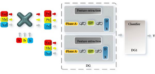
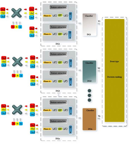
Prior to conducting feature extraction for islanding detection, it is crucial to perform multiple case studies to generate training data for the CatBoost classifier. These case studies involve simulating various scenarios using the DIgSILENT Power Factory software, including islanding and nonislanding events applied to a specific distributed system which will be discussed in the following sections. Table 2 outlines the specific types of disturbances and their corresponding output targets for the classifier. During the simulation of disturbances, measurements are recorded at the terminals of the DG units, encompassing measurements of three-phase voltage and instantaneous power for each phase. The GT methodology is employed to construct feature vectors from the signals originating from phase A. These feature vectors are employed as input parameters for the CatBoost classifier, a visual representation of which is provided in Figure 5. The classifiers leverage a dataset comprising 442 samples, which has been partitioned into separate training and testing sets. The allocation of these samples is shown in the development of the islanding detection algorithm. Seventy-five percent of the total samples, amounting to 338, are utilized for training and validation purposes. The remaining 25%, equivalent to 104 samples, are reserved for testing the performance of the algorithm. Through these rigorous case studies and data allocation, the proposed islanding detection algorithm is trained and evaluated, ensuring its effectiveness and reliability in detecting islanding events.

Table 2. Classifier outputs.

Event type	Target (Y)
Normal operation	1
Capacitor switching	2
Load switching	3
Disconnection events	4
Island event	5
Phase to phase fault	6
Three-phase fault at DG2	7
Line to ground fault at PCC	8

Abbreviation: PCC, point of common coupling.

3.2. Feature Extraction

The process of extracting features plays a crucial role in the development of islanding detection systems that rely on multiple parameters. The proposed Gabor feature is intended to discern the distinct characteristics of the voltage and instantaneous power signals for each phase. The utilization of GT for signal processing yields significant variables, namely, Gabor Matrix GM_{ij} and GC_{ij}, where i represents the time shift in samples and j denotes the number of channels [34]. These variables are instrumental in distinguishing islanding events from other events. Consequently, a total of five distinct characteristics are derived from both GM and GC. The calculation of GC can be achieved by utilizing Equation (8), followed by the generation of a time–frequency depiction of the DGT. The GC matrix consists of index values that correspond to individual frequency components at a specific moment in time. For instance, during standard operation, the index value representing the fundamental frequency is 17.6055. However, in an alternative scenario, this value may vary. Table 3 provides a depiction of certain variables, while Table 4 outlines the chosen features.

Table 3. Gabor variables.

Symbol	Description
D	Index value of Gabor coefficient

R = max (abs (GM))	Maximum values of the absolute value of Gabor matrix

Table 4. Gabor features.

Feature	Description
F1	The minimum value of D for the instantaneous power signal during the disturbance

F2	The maximum value of D for the instantaneous power signal during the disturbance

F3	The minimum value of D for the voltage signal during the disturbance

F4	The maximum value of D for the voltage signal during the disturbance

F5	The mean value of R for the voltage signal during the disturbance

Minimum and maximum features of D during the disturbance can be acquired within a specific time frame and a designated frequency range. Concurrently, the characteristics possessing an average value of R can be computed utilizing the following formula:

(22)

where n is the total number of samples. The proposed islanding detection process involves the application of the generalized transform GT technique for feature extraction from the instantaneous power per phase and voltage waveforms. To exemplify this concept, an illustration is provided for a single-phase fault occurring at a DG unit within a distribution system. In Figure 6a, the three-phase power is measured, then the instantaneous power signal for phase A is depicted as shown in Figure 6b, and this signal is subject to processing using the GT technique, resulting in the representation shown in Figure 6c. Similarly, in Figure 7a, the three-phase voltage is measured, and then the voltage signal for the phase is constructed as described in Figure 7b, which undergoes GT processing, leading to the representation shown in Figure 7c. By referring to Figures 6c and 7c, the minimum and maximum values of feature D can be obtained within a specific time frame and frequency range. Furthermore, the arithmetic average of feature R can be computed as provided in Figure 8. These derived features, such as minimum, maximum, and average values of D and R, capture the distinct characteristics of the disturbance event. They serve as essential inputs for the subsequent stages of the islanding detection algorithm, enabling accurate classification and differentiation of islanding events from other types of disturbances in power systems.

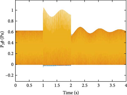
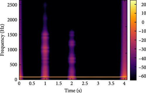
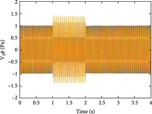
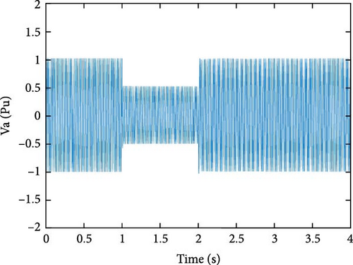
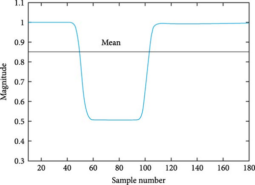
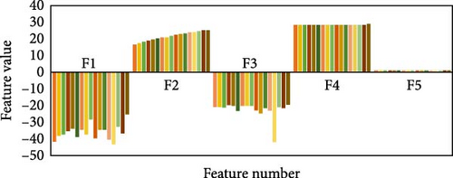
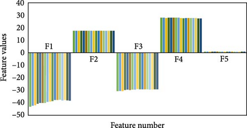
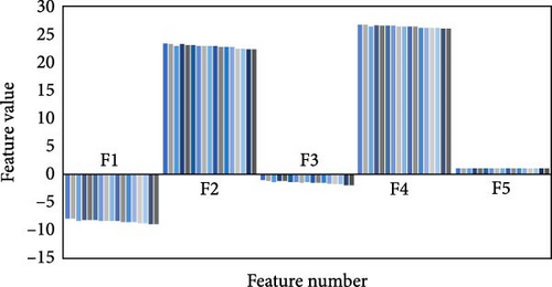
Through the implementation of diverse islanding and nonislanding events, a comprehensive spectrum of feature values can be acquired for each event category. In Figure 9, the input features and their associated values are presented, which are instrumental in event detection using the GT approach for the specific target DG. The feature values for islanding events (Figure 9a) exhibit distinct ranges, such as −41.7669 to −25.1491 for F1, 16.4839–25.2006 for F2, −41.7984 to −19.4178 for F3, 28.0043–28.4485 for F4, and 0.9999–1.0001 for F5. These ranges differ significantly from nonislanding occurrences, such as phase-to-phase fault events and capacitor bank switching events (depicted in Figure 9b,c). For example, the values of the features associated with capacitor bank switching events range from −43.5031 to −37.5772 for F1, 17.642–17.6945 for F2, −30.8625 to −29.208 for F3, 27.6016–28.3354 for F4, and 1.0014–1.0035 for F5. Similarly, the values of the features related to phase-to-phase fault events range from −8.8438 to −7.9587 for F1, 22.2778–23.359 for F2, −1.893 to −1.0344 for F3, 25.9814–26.7486 for F4, and 0.9652–0.9654 for F5. These distinct feature value combinations and ranges provide valuable insights for differentiating between islanding and nonislanding occurrences. By incorporating these distinctive case attributes, such as islanding and nonislanding events, the intelligent classification models can be effectively trained and utilized for accurate detection and classification.

3.3. Performance Evaluation Methods

In order to effectively gauge the potency and precision of the proposed islanding detection technique, performance evaluation is crucial. This process enables the evaluation of a machine learning model’s performance on an unseen dataset, often referred to as the testing dataset. For the purpose of measuring the efficiency of the islanding detection and classification, a host of metrics have been utilized, including the following.

3.3.1. Accuracy

This is one of the fundamental metrics used in machine learning. It quantifies the proportion of accurate predictions made by the model out of all predictions. Accuracy is most useful when the target classes are well balanced. The formula is as follows:

(23)

3.3.2. Precision

Precision is a measure that tells us what proportions of predicted positive instances are truly positive. Macroprecision calculates the score separately for each class and then takes the average, treating all classes equally. It is used when we need to treat each class equally:

(24)

where TP is true positive and FP is false positive.

3.3.3. Recall

Recall is a measure that tells us what proportions of actual positive instances were identified correctly. Macrorecall calculates the score separately for each class and then takes the average, treating all classes equally. It is used when we need to treat each class equally:

(25)

where FN is false negative.

3.3.4. F1 Score

The F1 score can be interpreted as a weighted average of the precision and recall, where an F1 score reaches its best value at 1 and worst score at 0:

(26)

3.3.5. Log Loss

Logarithmic loss (related to cross-entropy) measures the performance of a classification model where the prediction input is a probability value between 0 and 1. The goal of our machine learning models is to minimize this value:

(27)

where N is the number of samples, y_i is the actual value, and

is the estimated value.

3.3.6. Area Under the Curve (AUC) (One Versus Rest)

Receiver operating characteristic–AUC (ROC-AUC) is a performance measurement for classification problem at various threshold settings. It tells how much the model is capable of distinguishing between classes. As described in Table 5, the higher the AUC, the better the model is at predicting 0 s as 0 s and 1 s as 1 s.

Table 5. Scale of judgment of the AUC.

AUC	Judgment of prediction
1	Demonstrate accurate distinguishing among all the points within the class

0	Identify all the incorrectly assigned class points

0.5 < AUC < 1	High chance of accurately distinguishing between class points

Abbreviation: AUC, area under the curve.

Understanding the significance of each of these metrics in different contexts helps in optimizing and adjusting machine learning models for specific needs. Feature importance is an invaluable instrument that aids in understanding the model and optimizing the data preprocessing phase to enhance the accuracy of the model. The significance of features can be derived and understood through these metrics.

4. Design of the Artificial Intelligence Classifiers

The implementation of DT-based classifiers such as the RF necessitates the inclusion of appropriate hyperparameter sets, as well as the division of data into training and testing portions during the preprocessing stage. This is crucial for optimal performance. The previous sections have elucidated the characteristics of the GT that can be employed as input for the classifier, covering a range of disturbance events. The requirement for the number of classifiers is contingent upon the quantity of DG units interfaced with the network. Consequently, the proposed approach exhibits the potential for implementation in expansive distribution networks housing numerous DG units, with each DG unit equipped with an individual intelligent classifier. The development of each classifier can adhere to the process delineated in Figure 10. All models’ algorithms have been utilized as an islanding detection classifier within a Jupyter Notebook environment. The classifiers have been designed using default setting parameters to ensure a fair comparison. Concurrently, identical training and testing data sets are employed to construct all classifiers. Table 6 presents a visual representation of the function names and initialization parameters that are utilized for the classifiers in the designated DG.

Table 6. The parameter settings of the AI classifiers for the target DG.

Parameter setting	MLP1	MLP2	MLP3	RandomForest	DecisionTree	CatBoost	XGBoost	LightGBM
Main package	sklearn.neural_network			sklearn.ensemble	sklearn.tree	CatBoost.CatBoostClassifier	xgboost.XGBClassifier	lightgbm.LGBMClassifier

Training data (training intrinsic)	256 × 5

Validation data (training intrinsic)	82 × 5

Testing data	104 × 5

Iterations/estimators	max_iter = 300			n_estimators = 50	N/A	Iterations = 1000 n_estimators = 1000		n_estimators = 100

Accuracy metric	F1 score, accuracy, precision, recall, ROC-AUC, log loss

Tree/layer arch	Hidden layers = (100, 50)	Hidden layers = (100, 100, 50)	Hidden layers = (100, 100, 100, 50)	Tree depth = none		Tree depth = 6 Tree depth = 6		Tree depth = −1

Supports missing values?	No			Yes

Supports categorical features?	No					Yes	No	Yes

Needs feature scaling?	Yes			No

Model parallelism applied?	No			Yes	No	Yes

Handle imbalanced dataset?	No					Yes

Abbreviations: AI, artificial intelligence; DG, distributed generation; ROC-AUC, receiver operating characteristic–area under the curve.

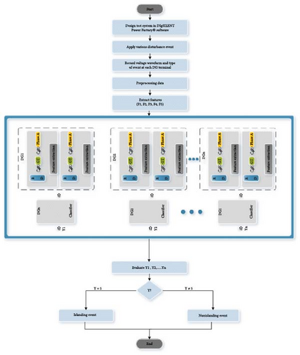
The proposed approach can be succinctly summarized in terms of its implementation phases, which are visually depicted in Figure 11:

Step 1:
Utilize the DIgSILENT Power Factory software to construct the testing system.
Step 2:
Execute a diverse array of power quality scenarios, encompassing islanding events and nonislanding events, by utilizing the simulation model.
Step 3:
Gather voltage and instantaneous power data for each phase signal at every DG terminal throughout the entirety of the simulated disturbance events. These events are distinctly categorized and identified by the predefined event class identifier as outlined in Table 2.
Step 4:
Extract the selected features using the GT technique as described previously.
Step 5:
Train the classifiers using the training data including the GT features. The present study employed nine distinct classifiers. The training component is executed through a process that occurs offline. These classifiers have the capacity to generate a collective of eight outputs. The specific quantity of classifiers utilized corresponds to the number of DG units integrated into the test system model.
Step 6:
For any new input, utilize the trained network to identify and classify the type of event.

5. Studied System

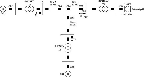
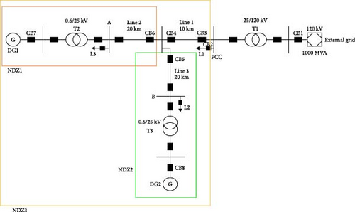
The proposed methodology for detecting islanding is validated using a radial distribution system comprising two DG units that are identical, as presented in reference [35]. The system configuration is depicted in Figure 12. The power system is energized by a 120 kV, 1000 MVA source operating at a frequency of 50 Hz. The simulation of DG units is carried out through the utilization of synchronous machines, which are situated within a 30 km radius of a distribution π-sections line model. The system under investigation is described in Table 7. The system under examination has been replicated and emulated through the framework illustrated in Figure 12, utilizing DIgSILENT Power Factory software. The voltage and current signals are obtained at the specified DG site for both islanding and nonislanding events, as well as other disturbances. The simulations encompass the subsequent scenarios:

Table 7. Parameters of the studied system.

Parameter	Description
External grid	120 kV, 1000 MVA
L1	15 MW and 3 MVar
L2 and L3	8 MW and 3 MVar
DG1 and DG2	1200 Vdc
T1	Transformer 120/25 kV
T2 and T3	Transformer 25/0.6 kV
Line 1	25 kV with 10 km
Line 2 and Line 3	25 kV with 20 km
PCC	Point of common coupling
A and B	The point nearby the respective DG (A is a point near DG1; B is a point near DG2)

Abbreviations: DG, distributed generation; PCC, point of common coupling.

1.
Load and capacitor switching at different locations
2.
Different faults at various locations
3.
Loss of main supply at the PCC bus
4.
Islanding condition
5.
Tripping of other DGs apart from the target one
6.
Breaker and recloser tripping events

The DIgSILENT Power Factory software is utilized to model the associated circumstances across a range of operational configurations, encompassing typical DG loading, minimum DG loading, maximum DG loading, and the diverse DG operating points that result in NDZ. The radial distribution system with two identical DGs can be subjected to testing using three distinct NDZ conditions, as illustrated in Figure 13. The testing involves the manipulation of loading setpoints by both the consumers and the DGs.

6. Results

This section presents the outcomes acquired through the implementation of the suggested islanding detection algorithm. It also compares these outcomes with those obtained through the application of traditional approaches. A variety of classifiers, including CatBoost, XGBoost, LightGBM, RandomForest, ExtraTrees, DecisionTree, and MLP (with three different configurations), have been employed in conjunction with proposed instantaneous power per phase and GT as input features. Table 2 displays the diverse categories of events that are produced by each classifier. Consequently, the assessment of whether an event satisfies the conditions for an islanding or nonislanding state is ascertained by applying supplementary if–then regulations to the outputs of each classifier, as illustrated as follows:

(28)

Yout denotes the output of the classifier. As per the equation, an event will be classified as a nonlanding event if the classifiers corresponding to both DG1 and DG2 do not match the specified event class (target) number 5. If the classifier records a class number of 5 for an event, it is classified as an islanding event. The evaluative process of the classifiers was conducted through an analysis of error metrics and decision accuracy.

6.1. Result of GT With the Best MLP Classifier

The examination in this study was focused on the performance of a specific MLP classifier named MLP3, alongside GT features, for the detection and classification of islanding. The evaluation was carried out on multiple datasets following offline training. The tests included a wide range of disturbance scenarios, both islanding and nonislanding events, under typical conditions and within the NDZ. Compared to the other two versions of MLP, MLP1 and MLP2, MLP3 has a more complex architecture with larger hidden layers, providing it with potentially more expressive power. However, its training time was not significantly different, thanks to the efficiency of the underlying optimization algorithms. The precision of the MLP3 classifier was evaluated by juxtaposing the output of the MLP3 classifier with the actual target values. Based on the data represented in Table 8, MLP3 classifier can identify a 59.3% of the nonislanding events, while for the nonislanding events, the accuracy stands at a specific value about 25% with a training time of 1.4 s.

Table 8. Results of the best MLP classification with Gabor transform features.

Classes	Number of scenarios	Number of sample data
Classes	Number of scenarios	Correct detection	Accuracy (%)
Nonislanding	96	57	59.3
Islanding	8	2	25

6.2. Result of GT With the Best DT-Based Model Classifier

By employing analogous methodologies that incorporate GT characteristics in conjunction with an MLP classifier, the MLP is substituted with the best DT-based model, namely, ExtraTrees classifier and subsequently trained and evaluated using GT features. The testing outcomes encompass identical disturbance scenarios, comprising islanding and nonislanding incidents while operating under both normal and NDZ configurations. The set of five distinct features, denoted as F1, F2, F3, F4, and F5, is each assigned a corresponding variable x (0), x (1), x (2), x (3), and x (4), respectively. The ExtraTrees classifier’s training duration is 1.31 s. Subsequently, the ExtraTrees classifier’s output outcomes are juxtaposed with the projected or factual target values. As described in Table 9, the classifier exhibits a 100% detection rate for the islanding classes. In the case of nonislanding events, the precision level is 97.9%.

Table 9. Results of ExtraTrees classification with Gabor transform features.

Classes	Number of cases	Number of sample data
Classes	Number of cases	Correct detection	Accuracy (%)
Nonislanding	96	94	97.9
Islanding	8	8	100

6.3. Result of GT With the Best Gradient Boosting Model

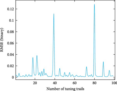
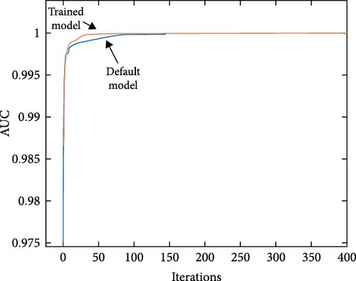
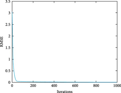
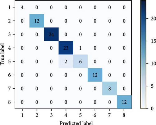
In an effort to bolster the performance of the islanding detection algorithm when integrated with the existing classifiers, the MLP and RF classifiers have been substituted with a CatBoost model. This transition maintains the utilization of the same training and testing data. The proposed method encompasses two models. The first model was established with default configurations, while the second model underwent an optimization process, which entailed the selection of optimal hyperparameters, specifically tree depth, learning rate, and the number of iterations. The previous result was attained by employing the randomized search algorithm available in scikit-learn, wherein each trial was executed with four cross-validation folds. Table 10 provides an overview of the accuracy achieved by the GT feature selection technique in conjunction with the CatBoost classifier. It also offers a comparative assessment of the resulting output against the target data, allowing for performance evaluation. The classifier exhibits a 100% detection rate for the cases on the island. The precision rate for nonislanding occurrences is 98.9%. The optimal hyperparameter configurations of the fine-tuned model are illustrated in Figure 14. The comparison between the two models involved the use of the AUC metric. In Figure 15, we can observe the CatBoost model with its default configuration, depicted by the blue line, and the meticulously tuned model, illustrated by the red line. It is noteworthy that the optimized model reached an AUC value of 1, a perfect score, after approximately 65 iterations. This finding demonstrates the effectiveness of the optimization process. However, it is necessary to perform additional iterations for the default model to achieve an AUC of 1. The duration required for training is estimated to be around 0.88 s, which is comparatively lower than the training times of other classifiers. The analysis of feature importance in CatBoost reveals that, in the training process of the fine-tuned model, key features include F1, F2, and F5, which contribute significantly at 23.27%, 22.28%, and 23.24%, respectively. In contrast, F3 and F4 make fewer substantial contributions at 19.6% and 11.59%, respectively. Figure 16 depicts the root mean square error (RMSE) binary metric for 1000 iterations of the optimized model. In Figure 17, the confusion matrix reveals strong predictive accuracy for classes 3, 4, and 6, with notable misclassifications for classes 5 and 7. The majority zeroes in nondiagonal cells indicate clear class distinctions, although some confusion between classes 5, 4, and 6 is evident. This suggests the model’s effectiveness with certain classes while highlighting potential areas for improvement.

Table 10. Results of CatBoost classification with Gabor transform features.

Classes	Number of scenarios	Sample data number
Classes	Number of scenarios	Correct detection	Accuracy (%)
Nonislanding	96	95	98.9
Islanding	8	8	100

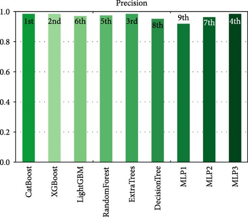
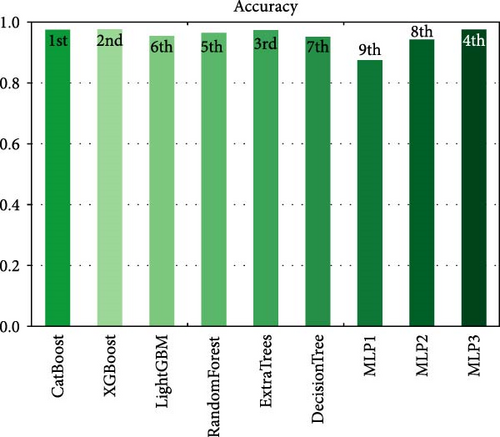
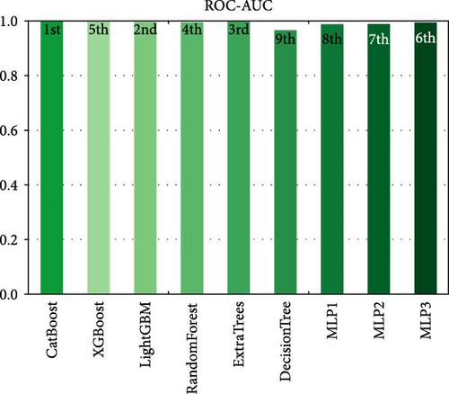
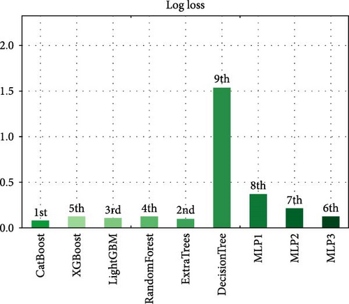
The results of the model evaluation are presented in Table 11. The table provides an overview of the performance metrics, including precision, accuracy, ROC-AUC, F1 score, log loss, and recall as shown in Figures 18–23, respectively, for each of the evaluated models. Among the models, CatBoost, ExtraTrees, and MLP3 achieved the highest accuracy scores, all exceeding 97%. These models demonstrated a strong ability to classify instances correctly. Similarly, they exhibited high precision, recall, and F1 score values, indicating their effectiveness in both positive and negative class predictions. In terms of the ROC-AUC metric, all models achieved impressive results, with values ranging from 0.998 to 1.000. This suggests that the models can effectively discriminate between different classes and have high predictive power. Notably, CatBoost achieved a perfect ROC-AUC score of 1.000, indicating its exceptional discriminative ability. The log loss metric measures the model’s calibration and uncertainty estimation. Lower log loss values indicate better model performance. In this regard, MLP3 achieved the lowest log loss among all models, followed by MLP2 and ExtraTrees. These models demonstrated superior calibration and accurate probability estimates. It is worth noting that DT and MLP1 obtained slightly lower scores in terms of accuracy, precision, recall, F1 score, and ROC-AUC compared to the other models. However, they still exhibited reasonably good performance, indicating their potential usefulness in certain scenarios. Overall, the evaluation results demonstrate that the models, particularly CatBoost, ExtraTrees, and MLP3, are highly capable of accurately detecting and classifying islanding events.

Table 11. Comparison between the classifiers’ performance.

Model	Accuracy	Precision	Recall	F1 score	ROC-AUC	Log loss
CatBoost	0.977528	0.986111	0.964286	0.971814	1	0.09272
XGBoost	0.977528	0.986111	0.964286	0.971814	0.998048	0.129105
LightGBM	0.955056	0.975	0.945055	0.954861	0.999136	0.115104
RandomForest	0.966292	0.977183	0.951786	0.960605	0.998369	0.121602
ExtraTrees	0.977528	0.986111	0.964286	0.971814	0.999129	0.107108
DecisionTree	0.955056	0.955532	0.943973	0.948582	0.96869	1.552305
MLP1	0.876404	0.921528	0.876717	0.88849	0.990203	0.374481
MLP2	0.94382	0.964461	0.930804	0.93984	0.991334	0.217469
MLP3	0.977528	0.986111	0.964286	0.971814	0.996206	0.135801

Abbreviation: ROC-AUC, receiver operating characteristic–area under the curve.

7. Conclusion

The present study introduced a novel algorithm that utilizes the GT method or feature extraction from both phase-specific instantaneous power and voltage waveforms. The primary objective of this approach is the precise classification of islanding and nonislanding events occurring at a designated DG site. The proposed methodology is assessed by employing multiple disturbance signals, including islanding operational states and different nonislanding network states, such as fluctuations in DG power, faults, load switching, capacitor switching, and NDZ conditions. The outcomes of the conducted tests conclusively demonstrate that the algorithm designed for islanding detection excels in its capacity to precisely identify and detect instances of islanding. To validate the effectiveness of the method, a comprehensive comparison is conducted, pitting it against a conventional approach involving eight distinct classifiers. The comparison reveals that the proposed detection method, featuring the combination of CatBoost and GT features, achieves an impressive accuracy rate of 98.9% in the detection of islanding regions. In contrast, the approach involving ExtraTrees and GT features attains a commendable accuracy of 97.7%. However, MLP3 in conjunction with GT features reaches a lower accuracy rate of 59.3%. Furthermore, the results unequivocally underscore the superior performance of the CatBoost classifier over the other classifiers employed in the evaluation. Moreover, the performance was evaluated using some metrics, and the GT with CatBoost classifiers was found to be more accurate than the GT technique with other classifiers. The CatBoost model is further improved by performing a hyperparameters tuning with more accurate results captured. The proposed methodology can be used for detection of islanding in which it can avoid and prevent dangerous situations and protect the stability of the system and the connected grid after restoration.

Conflicts of Interest

The authors declare no conflicts of interest.

Funding

This research was not funded by any organization or university.

Acknowledgments

The authors express their sincere gratitude for the support provided by the Department of Electrical and Communication Engineering, United Arab Emirates University, Al Ain, United Arab Emirates.

Open Research

Data Availability Statement

The data presented in this study are available on request from the corresponding author.

References

1 Cebollero J. A., Cañete D., Martín-Arroyo S., García-Gracia M., and Leite H., A Survey of Islanding Detection Methods for Microgrids and Assessment of Non-Detection Zones in Comparison With Grid Codes, Energies. (2022) 15, no. 2, https://doi.org/10.3390/en15020460, 460.
10.3390/en15020460
Web of Science® Google Scholar
2 Chanaa F., et al.Islanding Detection Method of a Photovoltaic Installation Destined to Power a RLC Load and Integrated to LV Network, International Journal of Intelligent Engineering and Systems. (2021) 14, no. 4, 299–311, https://doi.org/10.22266/ijies2021.0831.27.
10.22266/ijies2021.0831.27
Google Scholar
3 Abu Sarhan M., An Extensive Review and Analysis of Islanding Detection Techniques in DG Systems Connected to Power Grids, Energies. (2023) 16, no. 9, https://doi.org/10.3390/en16093678, 3678.
10.3390/en16093678
Google Scholar
4 Hussain A., Kim C. H., and Mehdi A., A Comprehensive Review of Intelligent Islanding Schemes and Feature Selection Techniques for Distributed Generation System, IEEE Access, 2021, 9, Institute of Electrical and Electronics Engineers Inc, 146603–146624.
10.1109/ACCESS.2021.3123382
Google Scholar
5 Jang S.-I. and Kim K.-H., An Islanding Detection Method for Distributed Generations Using Voltage Unbalance and Total Harmonic Distortion of Current, IEEE Transactions on Power Delivery. (2004) 19, no. 2, 745–752, https://doi.org/10.1109/TPWRD.2003.822964, 2-s2.0-1942439910.
10.1109/TPWRD.2003.822964
Web of Science® Google Scholar
6 Zeineldin H. H., El-Saadany E. F., and Salama M. M. A., Impact of DG Interface Control on Islanding Detection and Nondetection Zones, IEEE Transactions on Power Delivery. (2006) 21, no. 3, 1515–1523, https://doi.org/10.1109/TPWRD.2005.858773, 2-s2.0-33745602488.
10.1109/TPWRD.2005.858773
Web of Science® Google Scholar
7 Dube A. and Sindhu A., Comparative Analysis of Passive Islanding Detection Methods for Grid-Connected Distrubted Generators, 2015, Institute of Electrical and Electronics Engineers, https://doi.org/10.1109/INDICON.2015.7443138, 2-s2.0-84994310928.
10.1109/INDICON.2015.7443138
Google Scholar
8 Ozgonenel O., Karagol S., Ozgonenel O., and Karagol S., Islanding Detection in Photo-Voltaic Systems Based on Instantaneous Power Measurements, International Journal of Renewable Energy Research. (2017) 7, no. 4, 1723–1730.
Google Scholar
9 Zheng T., Yang H., Zhao R., Kang Y. C., and Terzija V., Design, Evaluation and Implementation of an Islanding Detection Method for a Micro-Grid, Energies. (2018) 11, no. 2, https://doi.org/10.3390/en11020323, 2-s2.0-85054924811, 323.
10.3390/en11020323
Web of Science® Google Scholar
10 Harirchi F., Hadidi R., Babakmehr M., and Simoes M. G., Advanced Three-Phase Instantaneous Power Theory Feature Extraction for Microgrid Islanding and Synchronized Measurements, 2019 International Conference on Smart Grid Synchronized Measurements and Analytics (SGSMA), 2019, College Station, TX, USA, IEEE, 1–8, https://doi.org/10.1109/SGSMA.2019.8784694, 2-s2.0-85071394297.
10.1109/SGSMA.2019.8784694
Google Scholar
11 Merlin V. L., Santos R. C., Grilo A. P., Vieira J. C. M., Coury D. V., and Oleskovicz M., A New Artificial Neural Network Based Method for Islanding Detection of Distributed Generators, International Journal of Electrical Power & Energy Systems. (2016) 75, 139–151, https://doi.org/10.1016/j.ijepes.2015.08.016, 2-s2.0-84941896271.
10.1016/j.ijepes.2015.08.016
Web of Science® Google Scholar
12 Kumar S. A., Subathra M. S. P., and Kumar N. M., et al.A Novel Islanding Detection Technique for a Resilient Photovoltaic-Based Distributed Power Generation System Using a Tunable-Q Wavelet Transform and an Artificial Neural Network, Energies. (2020) 13, no. 16, https://doi.org/10.3390/en13164238, 4238.
10.3390/en13164238
Web of Science® Google Scholar
13 Li S., Rodolakis A. J., El-Arroudi K., and Joós G., Islanding Protection of Multiple Distributed Resources Under Adverse Islanding Conditions, IET Generation, Transmission & Distribution. (2016) 10, no. 8, 1901–1912, https://doi.org/10.1049/iet-gtd.2015.1105, 2-s2.0-84969718632.
10.1049/iet-gtd.2015.1105
Web of Science® Google Scholar
14 Azim R., Li F., Xue Y., Starke M., and Wang H., An Islanding Detection Methodology Combining Decision Trees and Sandia Frequency Shift for Inverter-Based Distributed Generations, IET Generation, Transmission & Distribution. (2017) 11, no. 16, 4104–4113, https://doi.org/10.1049/iet-gtd.2016.1617, 2-s2.0-85035060409.
10.1049/iet-gtd.2016.1617
Web of Science® Google Scholar
15 Zielinski T. P., Joint Time-Frequency Resolution of Signal Analysis Using Gabor Transform, IEEE Transactions on Instrumentation and Measurement. (2001) 50, no. 5, 1436–1444, https://doi.org/10.1109/19.963221, 2-s2.0-0035483534.
10.1109/19.963221
Web of Science® Google Scholar
16 Subhi Suleiman M. K., An Intelligent Passive Islanding Detection and Classification Scheme for a Radial Distribution SysteM, 2022, United Arab Emirates University, MS thesis.
Google Scholar
17 Hirofumi A., Edson W., and Mauricio A., Instantaneous Power Theory and Applications to Power Conditioning, 2017.
Google Scholar
18 Cho S. H., Jang G., and Kwon S. H., Time-Frequency Analysis of Power-Quality Disturbances via the Gabor–Wigner Transform, IEEE Transactions on Power Delivery. (2010) 25, no. 1, 494–499, https://doi.org/10.1109/TPWRD.2009.2034832, 2-s2.0-73849103893.
10.1109/TPWRD.2009.2034832
Web of Science® Google Scholar
19 Cheng J.-Y., Huang S.-J., and Hsieh C.-T., Application of Gabor-Wigner Transform to Inspect High-Impedance Fault-Generated Signals, International Journal of Electrical Power & Energy Systems. (2015) 73, 192–199, https://doi.org/10.1016/j.ijepes.2015.05.010, 2-s2.0-84929610519.
10.1016/j.ijepes.2015.05.010
Web of Science® Google Scholar
20 Szmajda M., Górecki K., and Mroczka J., Gabor Transform, Gabor-Wigner Transform and SPWVD as a Time-Frequency Analysis of Power Quality, ICHQP. 2010—14th International Conference on Harmonics and Quality of Power. (2010) 56, 8, https://doi.org/10.1109/ICHQP.2010.5625371, 2-s2.0-78650563598, 25371.
10.1109/ICHQP.2010.5625371
Google Scholar
21 LTFAT Reference Manual, LTFAT: The Large Time-Frequency Analysis Toolbox [online].[cit], 2017.
Google Scholar
22 Friedman J. H., Stochastic Gradient Boosting, Computational Statistics & Data Analysis. (2002) 38, no. 4, 367–378, https://doi.org/10.1016/S0167-9473(01)00065-2, 2-s2.0-0037186544.
10.1016/S0167-9473(01)00065-2
Web of Science® Google Scholar
23 Dorogush A. V., Ershov V., and Gulin A., CatBoost: Gradient Boosting With Categorical Features Support, 2018.
Google Scholar
24 Pargent F., Pfisterer F., Thomas J., and Bischl B., Regularized Target Encoding Outperforms Traditional Methods in Supervised Machine Learning With High Cardinality Features, Computational Statistics. (2022) 37, no. 5, 2671–2692, https://doi.org/10.1007/s00180-022-01207-6.
10.1007/s00180-022-01207-6
Web of Science® Google Scholar
25 Potdar K., Taher S. P., and Chinmay D. P., Machine Learning With R: Learn How to use R to Apply Powerful Machine Learning Methods and Gain an Insight into Real-World Applications, International Journal of Computer Applications. (2017) 175, no. 4, 7–9, https://doi.org/10.5120/ijca2017915495.
10.5120/ijca2017915495
Google Scholar
26 Ghori K. M., Abbasi R. A., Awais M., Imran M., Ullah A., and Szathmary L., Performance Analysis of Different Types of Machine Learning Classifiers for Non-Technical Loss Detection, IEEE Access. (2020) 8, 16033–16048, https://doi.org/10.1109/ACCESS.2019.2962510.
10.1109/ACCESS.2019.2962510
Web of Science® Google Scholar
27 Muhammed M. M., Ibrahim A. A., Ridwan R. L., Abdulaziz R. O., and Saheed G. A., Comparison of the CatBoost Classifier With Other Machine Learning Methods, 2020, [Online]. Available: https://www.researchgate.net/publication/348277609.
Google Scholar
28 Ke G., Meng Q., and Finley T., et al.Lightgbm: A Highly Efficient Gradient Boosting Decision Tree, Advances in Neural Information Processing Systems, 2017, 30.
Google Scholar
29 Chen T. and Guestrin C., Xgboost: A Scalable Tree Boosting System, Proceedings of the 22nd Acm Sigkdd International Conference on Knowledge Discovery and Data Mining, 2016.
Google Scholar
30 Breiman Leo, Random Forests, Machine Learning, 2001, 45, 5–32.
Google Scholar
31 Geurts P., Ernst D., and Wehenkel L., Extremely Randomized Trees, Machine Learning, 2006, 63, 3–42.
Google Scholar
32 Popescu M.-C., Balas V. E., and Perescu-Popescu L., et al.Multilayer Perceptron and Neural Networks, WSEAS Transactions on Circuits and Systems. (2009) 579–588.
Google Scholar
33 Søndergaard P. L., Balazs P., and Dörfler M., et al. “LTFAT Reference Manual. LTFAT: The Large Time-Frequency Analysis Toolbox [online].[cit], 2017.
Google Scholar
34 Khamis A., Shareef H., Mohamed A., and Bizkevelci E., Islanding Detection in a Distributed Generation Integrated Power System Using Phase Space Technique and Probabilistic Neural Network, Neurocomputing. (2015) 148, 587–599, https://doi.org/10.1016/j.neucom.2014.07.004, 2-s2.0-84908069419.
10.1016/j.neucom.2014.07.004
Web of Science® Google Scholar
35 Khamis A., Shareef H., and Mohamed A., Islanding Detection and Load Shedding Scheme for Radial Distribution Systems Integrated With Dispersed Generations, IET Generation, Transmission & Distribution. (2015) 9, no. 15, 2261–2275, https://doi.org/10.1049/iet-gtd.2015.0263, 2-s2.0-84947435352.
10.1049/iet-gtd.2015.0263
Web of Science® Google Scholar

All articles

An Effective Islanding Detection Method for Distributed Generation Integrated Power Systems Using Gabor Transform Technique and Artificial Intelligence Techniques

Abstract

1. Introduction

2. Proposed Islanding Detection Algorithm

2.1. Instantaneous Power Theory

2.2. GT

2.3. Implementation of Diverse Machine Learning Algorithms

2.3.1. Gradient Boosting Techniques

2.3.1.1. CatBoost Algorithm

2.3.1.2. LightGBM

2.3.1.3. XGBoost

2.3.2. DT

2.3.2.1. General DT Models

2.3.2.2. RF

2.3.2.3. ExtraTrees

2.3.3. MLP

3. Identifying the Islanding Detection Algorithm

3.1. Data Gathering for Training and Testing

3.2. Feature Extraction

3.3. Performance Evaluation Methods

3.3.1. Accuracy

3.3.2. Precision

3.3.3. Recall

3.3.4. F1 Score

3.3.5. Log Loss

3.3.6. Area Under the Curve (AUC) (One Versus Rest)

4. Design of the Artificial Intelligence Classifiers

5. Studied System

6. Results

6.1. Result of GT With the Best MLP Classifier

6.2. Result of GT With the Best DT-Based Model Classifier

6.3. Result of GT With the Best Gradient Boosting Model

7. Conclusion

Conflicts of Interest

Funding

Acknowledgments

Open Research

Data Availability Statement

References

Figures

References

Related

Information