In this paper, we applied an efficient integrative method called the fractional Picard method to find the approximate solution to a system of fractional algebraic differential equations (SFADEs). By comparing the results with the exact solution, it was found that this method is highly efficient for finding solutions. Also, a genetic algorithm (GA) was used to speed up the approximate solutions when choosing the best values for the fractional derivative, which increased the efficiency of Picard’s fractional integral method in finding the best solutions. The MATLAB program was used to find approximate solutions.

1. Introduction

The French mathematician Charles Emile Picard (1856–1941), whose name is often linked with the technique, made early and substantial contributions to the method’s systematic development of iterations for boundary and initial value issues in both ordinary and partial differential equations. Theory and application of the technique of iterations to differential equations have attracted a great deal of attention throughout the 20th century and beyond, and both have grown significantly [1]. Many researchers have dealt with the Picard method, either alone or with other methods, and we mention among them. The study [2] gives a comparison between Picard’s iteration method and the Adomian decomposition method (ADM) in solving nonlinear differential equations. In [3], homotopic perturbation and Picard techniques were employed to solve the fractional-time Schrödinger equations. In [4], the approximate solution of the fractional differential equations was discovered through the application of Picard′s iterative technique. In [5], they generalized Picard’s iterated approximation to solve the fractional differential equations with an initial condition. The article’s objective [6] is to expand the Boundary Value Problems Picard Method (BVPP) applications for ODES with nonlinear and Robin boundary conditions. While [7] studied a class of new Picard–Mann iteration processes. Also, the successive approximations method (Picard–Lindelof method) is applied to solve multipantograph delay equations and neutral functional-differential equations [8]. An inexact Picard iteration method (PIM), named Picard-SHSS, was suggested to solve the absolute value equation [9]. The predator–prey model with the numerical methods applied is the ADM and the PIM [10]. The paper [11] proposed an iterative scheme for the solution of second order fuzzy differential equations with fuzzy initial conditions using the fuzzy Picard method, and the convergence is also discussed under generalized H-differentiability. Picard iterative approach for the ψ−Hilfer fractional differential problem was solved in [12]. Picard’s iteration method has been submitted as a technique for solving initial value problems of the first and second order linear differential equations [13]. The Picard method for solving nonlinear quadratic Volterra integral equations using self-canceling noise terms was utilized in [14]. The differential equations arising in fractal heat transfer with a local fractional derivative were solved using the Picard Successive Approximation Method [15]. The PIM was applied to fractional quadratic Riccati differential equations [16].

Genetic algorithms (GAs) are types of optimization algorithms inspired by natural selection. A population of potential solutions is used for a problem, which iteratively evolves to find better solutions. The algorithm selects the fittest individuals in the population and uses them to create new individuals through recombination and mutation. Over time, the population evolves towards better solutions through a process of selection [17]. Many sciences and their branches have benefited from GAs to find and improve solutions to scientific problems that require optimal solutions [18–20].

The multiplicity and diversity of specializations in the field of fractional algebraic equations, such as quantum mechanics, as well as biomathematics, in addition to circuit systems, control systems, electric motors, and other fields that serve the rest of the sciences, put researchers in front of a great challenge to search for guaranteed methods to find solutions to these systems used in real applications, such as [21–24]. From this standpoint, the quest to find a simplified and available method was one of the most important challenges facing this manuscript that the technique relies essentially on a traditional process that was developed to obtain solutions close to the exact solution while preserving the properties of the algebraic equation, especially the values of the fractional derivative, which have an effective role when studying the behavior of these systems. There was another challenge lying in how to reach the optimal values for the fractional derivatives that make the approximate solutions close to the exact solution. For this reason, the idea of using the Picard fractional method to solve fractional algebraic systems and using the GA to find the optimal values was born, thus achieving the goal of the paper.

The vocabulary of our research consists of several sections. The next section contains an overview of Picard’s method with a definition and some properties of fractional integration. We continue with the third section, where the most important concepts and steps for applying the GA are presented to obtain the optimal values for the approximate solution, followed by an explanation of the basic steps for solving problems, and finally the application and results.

2. Picard Method and Fractional Integration Definition

Picard’s iterative approach assists in solving the differential equation as (y₁(x), y₂(x), y₃(x), ⋯, y_k(x)) to a solution where the nth approximate relies on the earlier approximations through a sequence of approximations. The precision of the solution will rise with repeated solving of the differential equation.

(1)

with initial condition y = y₀ at x = x₀.

Integrating both sides of Equation (1) produces

(2)

(3)

By starting iterations and replacing y = y₀, we get

(4)

(5)

For the iterative formula, Equation (3) will be written as

(6)

Now reviewing the proposed solution method, we combine Picard’s method with fractional integration to solve systems containing the fractional derivative, which requires not ignoring the values of the fractional derivative and preserving the properties of these systems.

Suppose that we have the initial value problem:

(7)

(8)

Let x(t) be a solution of Equations (7) and (8), and by integrating Equation (1), we get

(9)

To construct the solution, the Picard method is applied to Equation (9) to get the sequence:

(10)

(11)

for the unique solution of x and uniform convergence, in [25].

Definition 1. The Riemann–Liouville fractional integration of order α is defined as

(12)

With the properties of the Riemann–Liouville integral:

(13)

where α₁, α₂, λ₁, and λ₂ are constants [26].

3. GA

A GA, introduced by John Holland in 1970, has at least the following elements: chromosome combinations, selection for fitness, crossover to produce new offspring, and random mutation for new offspring. GA factor, so to speak, selection, is a factor that selects chromosomes in the population for reproduction. The greater the fitness of the chromosome, the more it will be selected. Crossover is an operator that selects a location to exchange sequences between two chromosomes to create offspring. The mutation is the operator that randomly turns some of the bits in a chromosome. The procedure for GAs contains the following steps [27, 28].

1.
Starting with a population of expected solutions.
2.
Assess the fitness of each chromosome by a fitness function.
3.
A neoteric population is produced from a sequence of concepts:
- a.
  Selection mechanism: selecting two chromosomes from the solution consequently to their fitness.
- b.
  Two chromosomes crossing over join their genetic material to produce new offspring.
- c.
  Mutation to maintain genetic diversity and extract new potential solutions.

This process is repeated, until following the generation of new offspring, a new population is created and assessed. Then, the previous population is replaced by this new one, and the process continues until the condition is fulfilled.

4.
Finally, after the best option for the present population is identified, the entire procedure can be restarted at step one to achieve even further optimization.

One of the most important features of the GA, which encourages researchers to use it, is that the method proposes solutions to the problem by improving the solutions across stages or generations. The algorithm uses the concept of individuals in the primary community as a potential solution. Then, it begins the process of enhancing solutions across more than one generation to find the best solution. As for the various swarm algorithms, for example, they depend mainly on the behavior of the individuals, the nature of their interaction, and the behaviors issued by each individual towards the other, which often lead to improving the performance of the swarm, that is, improving the solutions to achieve the goal of the problem. In short, the GA depends on successive stages (generations) to improve the solution, while swarm algorithms depend on the behaviors of individuals in the swarm.

4. The Basic Steps for the Solution

To solve any SFADEs using the Picard integral with a GA, we can summarize the proposed method with the following main steps:

(14)

(15)

Subject to initial conditions:

( )

First step: by fractional Picard iterative method, we get

(16)

Second step: the definition and properties of the rational derivative detailed in Section 2 are applied.

Third step: to produce the sequence of functions x₀(t), x₁(t), x₂(t), ⋯, we repeat the process n times until we obtain an approximate solution close to the exact solution. In this research, the MATLAB software was used to achieve the purpose.

Fourth step: to improve the solution and obtain the best values for (α_i), we use the GA and begin with specific values for the fractional derivative, which range between 0.1 and 0.9, then convert these values to the binary form, i.e., zeros and ones, as shown in Table 1.

Table 1. The results of converting α values from decimal to binary.

Decimal number	Binary number
0.1	0.00011001
0.2	0.00110011
0.3	0.01001100
0.4	0.01100110
0.5	0.10000000
0.6	0.10011001
0.7	0.10110011
0.8	0.11001100
0.9	0.11100110

Through this operation, the initial population is generated so that the steps mentioned in Section 3 on the selection processes continue to be applied. The intersection between the chromosomes (α_i) and the mutation process led to the selection of the best values for the fractional derivatives so that they give results close to the exact solution.

5. The Application on Selected Issues

By considering the following SFADEs, the method’s effectiveness will be examined. The results were calculated using MATLAB software.

Example 1. Let us have SFADEs [29].

(17a)

(17b)

(17c)

where 0 < α₁, α₂ < 1, with initial conditions x(t) = 0, y(t) = 0 and z(t) = 1.

The exact solutions are

(18)

Equation (17a) can be written in the form

(19)

(20)

(21)

(22)

(23)

(24)

(25)

(26)

(27)

From Equation (17b), we get

then

(28)

(29)

(30)

(31)

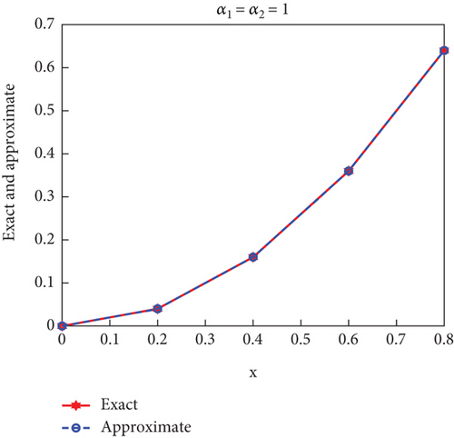
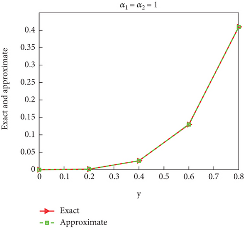
Case 1. Assume that α₁ = α₂ = 1.

(32)

(33)

(34)

(35)

Figure 1 expresses the results of the solution when α₁ = α₂ = 1, and it can be observed that the approximate and exact solutions coincide.

Case 2. In this case, the research sought to study the effect of the different value of α₁ and α₂ on the exact and approximate solution; suppose that α₁ = 0.6, α₂ = 0.4 and α₁ = 0.8, α₂ = 0.5, then the results appeared as in Figure 2.

Details are in the caption following the image — **Figure 1 (a)**
Open in figure viewer PowerPoint

The exact solution matches the approximate solution when α₁ = α₂ = 1 for (a) x values and (b) y values.

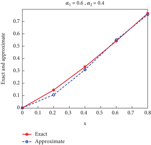
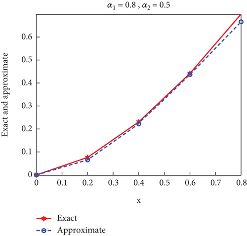
Let us focus on the effect of alpha values on each other and the results when the values are not optimal. Replacing the values of α₁ and α₂, an inverse relationship was found between their values, as shown in Figure 2 for the values x.

Seeking to make the approximate solutions close to the exact solution without eliminating the effect of the value of the fractional derivative, a GA was used to perform this task, the details of which are described in the fourth section, to arrive at the best alpha values that make the approximate solutions closer to the exact solutions, as shown in Figure 3.

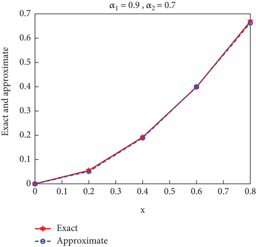
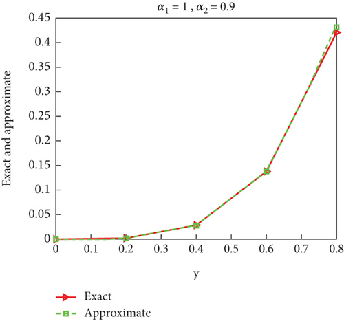
Tables 2 and 3 present the impact of the optimal values of α₁ and α₂ on the approximate solution for the values of x and y, respectively, and make it close to the exact solution, which preserves the fractional behavior of the system of algebraic equations. The results showed that the best value for x is when α₁ = 0.9, α₂ = 0.7 and the best value for y is when α₁ = 1, α₂ = 0.9.

Example 2. Another SFADEs [30]. By following the same steps implemented in the first example, the second is solved as follows:

(36a)

(36b)

(36c)

with initial conditions s(0) = q(0) = p(0) = 1.

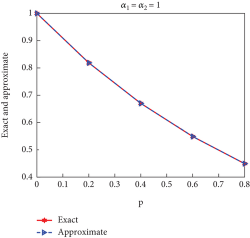
For α₁ = α₂ = 1, the exact solutions are s(t) = e^t, q(t) = e^2t, p(t) = e^−t.

Applying Picard’s definition, then

(37)

The expression for the first equation in the system (36a) is as follows:

(38)

(39)

By substituting the initial values and applying the fractional Riemann–Liouville derivative, we obtain

(40)

(41)

(42)

(43)

(44)

(45)

(46)

(47)

(48)

(49)

Case 3. If α₁ = α₂ = 1

(50)

(51)

Obviously, from Figure 4, the results for x and y are identical when α₁ = α₂ = 1.

Table 2. The results of both the exact and approximate solutions for x relative to the optimal values of the fractional derivative.

x	α₁	α₂	x_exact	x_approximate	\|x_exact − x_approximate\|
0	0.9	0.7	0	0	0
0.2			0.046984757723521	0.045317124246040	0.001667633477481
0.4			0.175353316221635	0.173969894157095	0.001383422064540
0.6			0.378867520493613	0.378203909305038	0.000663611188575
0.8			0.654441716840687	0.646620796327241	0.007820920513446

Table 3. The results of both the exact and approximate solutions y of relative to the optimal values of the fractional derivative.

y	α₁	α₂	y_exact	y_approximate	\|y_exact − y_approximate\|
0	1	0.9	0	0	0
0.2			0.001940869713876	0.001756583063930	0.000184286649946
0.4			0.028575429474892	0.027526929715363	0.001048499759528
0.6			0.137792903508991	0.137670240922619	0.000122662586373
0.8			0.420716117025556	0.431366939095611	0.010650822070055

As in the previous example, the GA was applied to obtain the best α values, and the results appeared as shown in Figure 5.

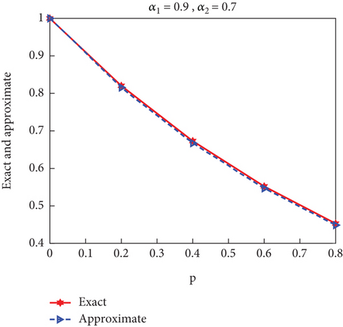
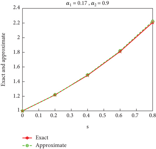
Tables 4 and 5 involve the details of the results for the values of p and s, respectively, when substituting the optimal values for the fractional derivatives α₁ and α₂.

Table 4. The results of p values with the optimal values of α₁ and α₂.

p	α₁	α₂	p_exact	p_approximate	\|p_exact − p_approximate\|
0	0.9	0.7	1.000000000000000	1.000000000000000	0
0.2			0.820369853137831	0.815557500672764	0.004812352465067
0.4			0.673006695937386	0.667312040880429	0.005694655056958
0.6			0.552114404306931	10.546855264192774	0.005259140114157
0.8			0.452938012776558	0.448688378047819	0.004249634728738

Table 5. The influences of the optimal values of α₁ and α₂ on s values.

s	α₁	α₂	s_exact	s_approximate	\|s_exact − s_approximate\|
0	1	0.9	1.000000000000000	1.000000000000000	0
0.2			1.218962393821643	1.221402947361165	0.002440553539522
0.4			1.485869317551390	1.491826785628538	0.005957468077148
0.6			1.811218820228573	1.822119710254121	0.010900890025548
0.8			2.207807628840633	2.225541787371441	0.017734158530808

6. Conclusion

Through this research, we can conclude the following points:

•
Using fractional integration with Picard’s method gave the best results for solving such systems of equations.
•
The values of α₁ and α₂ had an impact on the solution through an inverse relationship linking their values when finding the approximate solution by the method proposed in this research. It also has an impact on the values of each other, according to the equation. In the first example, the value of α₁ affected the values of α₂, but in the second example, the effect was not clear.
•
The GA played a major role in accelerating the finding of approximate solutions that are close to the exact solution by finding the best values for α₁ and α₂, which saved effort and time and increased the efficiency of the method in finding the best approximate solution.

Finally, it can be said that the research achieved its goal, which was to solve a system of fractional equations by mixing fractional integration and its properties with the Picard method and improving the results with intelligent techniques.

Conflicts of Interest

The authors declare no conflicts of interest.

Funding

The research was funded by the researchers, and they did not receive financial support from any party when preparing the research.

Open Research

Data Availability Statement

The information that backs up the study’s conclusions is always available to readers, when they ask.

References

1 Tisdell C. C., On Picard’s iteration method to solve differential equations and a pedagogical space for otherness, International Journal of Mathematical Education in Science and Technology. (2019) 50, no. 5, 788–799, https://doi.org/10.1080/0020739X.2018.1507051, 2-s2.0-85052088888.
10.1080/0020739X.2018.1507051
Web of Science® Google Scholar
2 Oludoun O., Adebimpe O., Gbadamosi B., and Abiodun O. E., On the comparison between Picard iteration method and Adomian decomposition method in solving non linear differential equations, Seria Informatică. (2019) 17, no. 4, 327–339.
Google Scholar
3 Eladdad E. E. and Aljawazneh S. M., Picard and Homotopy perturbation methods for solving the time-fractional schrödinger equations, Delta Journal of Science. (2020) 42, no. 1, https://doi.org/10.21608/djs.2020.139824.
10.21608/djs.2020.139824
Google Scholar
4 Yu C., Picard Iterative Method for Solving Fractional Differential Equations, International Journal of Computer Science and Information Technology Research. (2022) 10, no. 4, 17–23.
CAS Google Scholar
5 Al Masalmeh M., Solving conformable fractional differential equations using Picard’s iteration method, Journal of Mathematics and Computer Science. (2020) 10, no. 5, 1571–1581, https://doi.org/10.28919/jmcs/4688.
10.28919/jmcs/4688
Google Scholar
6 Filobello-Nino U., Alvarez-Gasca O., Contreras-Hernandez A. D., Palma-Grayeb B. E., Cuellar-Hernandez L., Mendez-Perez J. M., Pretelin-Canela J. E., Vazquez-Aguirre J. L., Jimenez-Fernandez V. M., Sampieri-Gonzalez C. E., Pereyra-Diaz D., Vazquez-Leal H., and Bagatella-Flores Facultad N., Modified Picard method for solving boundary value problems with nonlinear and Robin boundary conditions, International Journal of Engineering Research & Technology. (2019) 8, no. 12, 762–767, http://www.ijert.org/.
Google Scholar
7 Li T. F. and Lan H. Y., On new Picard-Mann iterative approximations with mixed errors for implicit midpoint rule and applications, Journal of Function Spaces. (2019) 2019, 13, https://doi.org/10.1155/2019/4042965, 2-s2.0-85063292829, 4042965.
10.1155/2019/4042965
Web of Science® Google Scholar
8 Jafari M. A., Aminataei A., Nasir K., and Aminataei A., Method of successive approximations for solving the multi-pantograph delay equations, General Mathematics Notes. (2013) 8, no. 1, 23–28, http://www.i-csrs.orgavailablefreeonlineat, http://www.geman.in.
Google Scholar
9 Miao S. X., Xiong X. T., and Wen J., On Picard-SHSS iteration method for absolute value equation, AIMS Mathematics. (2021) 6, no. 2, 1743–1753, https://doi.org/10.3934/math.2021104.
10.3934/math.2021104
Web of Science® Google Scholar
10 Anake T. A., Adeleke O. J., Edeki S. O., and Ejiogu J. I., Iterative methods for the solutions of a predator-prey model, WSEAS Transactions on Mathematics. (2019) 18, 161–167.
Google Scholar
11 Sindu Devi S. and Ganesan K., Fuzzy Picard’s method for derivatives of second order, Journal of Physics: Conference Series. (2018) 1000, no. 1, article 012038, https://doi.org/10.1088/1742-6596/1000/1/012038, 2-s2.0-85046707795.
10.1088/1742-6596/1000/1/012038
Google Scholar
12 Pawar E. D. and Dhaigude R. M., Picard iterative approach for ψ−Hilfer fractional differential problem, Journal of Mathematical Modeling. (2023) 11, no. 3, 573–585, https://doi.org/10.22124/jmm.2023.24626.2201.
10.22124/jmm.2023.24626.2201
Google Scholar
13 Science A., Picard fixed point iteration combined with integrating factor approach, Egyptian Journal of Pure and Applied Science. (2011) 49, no. 1, 71–78, https://doi.org/10.21608/ejaps.2011.186255.
10.21608/ejaps.2011.186255
Google Scholar
14 Ababneh O. Y. and Al-sawalha M. M., Picard approximation method for solving nonlinear quadratic Volterra integral equations, Journal of Mathematics Research. (2016) 8, no. 1, https://doi.org/10.5539/jmr.v8n1p79.
10.5539/jmr.v8n1p79
Google Scholar
15 Yang A. M., Zhang C., Jafari H., Cattani C., and Jiao Y., Picard successive approximation method for solving differential equations arising in fractal heat transfer with local fractional derivative, Abstract and Applied Analysis. (2014) 2014, https://doi.org/10.1155/2014/395710, 2-s2.0-84897789210, 395710.
10.1155/2014/395710
Google Scholar
16 Sceince J. O. F., An application of Picard iteration method to fractional quadratic Ricccati differential equations, Ilorin Journal of Science. (2018) 5, no. 2, 125–132, https://doi.org/10.54908/iljs.2018.05.02.004.
10.54908/iljs.2018.05.02.004
Google Scholar
17 Borghi G. and Pareschi L., Kinetic description and convergence analysis of genetic algorithms for global optimization, 2023, https://arxiv.org/abs/2310.08562.
Google Scholar
18 Xiao Y., Construction of a mathematical model based on a genetic algorithm for an aptitude program in high school student optimization, Revista Brasileira de Medicina do Esporte. (2022) 28, no. 5, 446–450, https://doi.org/10.1590/1517-8692202228052021_0537.
10.1590/1517-8692202228052021_0537
Web of Science® Google Scholar
19 Hussain E. A. and Abdul-Abbass Y. M., Solving differential equation by modified genetic algorithms, Journal of University of Babylon for Pure and Applied Sciences. (2018) 26, no. 10, 233–241, https://doi.org/10.29196/jubpas.v26i10.1877.
10.29196/jubpas.v26i10.1877
Google Scholar
20 Hamid A., Klebanov E. I., and Albermany S. A., Quantum fuzzy genetic algorithm with Turing to solve DE, Periodicals of Engineering and Natural Sciences. (2023) 11, no. 1, 41–47, https://doi.org/10.21533/pen.v11i1.3417.
10.21533/pen.v11i1.3417
Google Scholar
21 Arqub O. A., The reproducing kernel algorithm for handling differential algebraic systems of ordinary differential equations, Mathematicsl Methods in the Applied Sciences. (2016) 39, no. 15, 4549–4562, https://doi.org/10.1002/mma.3884, 2-s2.0-84969921257.
10.1002/mma.3884
Web of Science® Google Scholar
22 Karabacak M. and Çelik E., The numerical solution of Fractional Differential-Algebraic Equations (FDAEs) by Haar Wavelet functions, International Journal of Engineering and Applied Sciences (IJEAS). (2015) 2, no. 10.
Google Scholar
23 Tai Y., Chen N., Wang L., Feng Z., and Xu J., A numerical method for a system of fractional differential-algebraic equations based on sliding mode control, Mathematics. (2020) 8, no. 7, https://doi.org/10.3390/math8071134.
10.3390/math8071134
Google Scholar
24 Ghomanjani F. and Noeiaghdam S., Application of said ball curve for solving fractional differential-algebraic equations, Mathematics. (2021) 9, no. 16, https://doi.org/10.3390/math9161926.
10.3390/math9161926
Web of Science® Google Scholar
25 Bellman R., Existence and uniqueness theorems, Dynamic Programming, 2021, Princeton University Press, 116–151.
10.2307/j.ctv1nxcw0f.8
Google Scholar
26 Jasim S. M. N. and Ibraheem G. H., Fractional pantograph delay equations solving by the meshless methods, Ibn AL-Haitham Journal For Pure and Applied Sciences. (2023) 36, no. 3, 382–397, https://doi.org/10.30526/36.3.3076.
10.30526/36.3.3076
Google Scholar
27 Jouilik B., Daoudi J., Tajani C., and Abouchabaka J., Numerical optimization algorithm based on genetic algorithm for a data completion problem, TWMS Journal of Applied & Engineering Mathematics. (2023) 13, no. 1, 86–97.
Web of Science® Google Scholar
28 Al-Rozbayani A. M. and Qasim A. F., Modified α -parameterized differential transform method for solving nonlinear generalized gardner equation, Journal of Applied Mathematics. (2023) 2023, https://doi.org/10.1155/2023/3339655, 3339655.
10.1155/2023/3339655
Google Scholar
29 Ahmed H. F., Numerical study on factional differential-algebraic systems by means of Chebyshev pseudo spectral method, Journal of Taibah University for Science. (2020) 14, no. 1, 1023–1032, https://doi.org/10.1080/16583655.2020.1798071.
10.1080/16583655.2020.1798071
Web of Science® Google Scholar
30 Ibiş B. and Bayram M., Numerical comparison of methods for solving fractional differential–algebraic equations (FDAEs), Computers & Mathematics With Applications. (2011) 62, no. 8, 3270–3278, https://doi.org/10.1016/j.camwa.2011.08.043, 2-s2.0-80053370817.
10.1016/j.camwa.2011.08.043
Web of Science® Google Scholar

Citing Literature

All articles

Fractional Integration via Picard Method for Solving Fractional Differential-Algebraic Systems

Abstract

1. Introduction

2. Picard Method and Fractional Integration Definition

3. GA

4. The Basic Steps for the Solution

5. The Application on Selected Issues

6. Conclusion

Conflicts of Interest

Funding

Open Research

Data Availability Statement

References

Citing Literature

Figures

References

Information

About Wiley Online Library

Help & Support

Opportunities

Connect with Wiley

Fractional Integration via Picard Method for Solving Fractional Differential-Algebraic Systems

Abstract

1. Introduction

2. Picard Method and Fractional Integration Definition

3. GA

4. The Basic Steps for the Solution

5. The Application on Selected Issues

6. Conclusion

Conflicts of Interest

Funding

Open Research

Data Availability Statement

References

Citing Literature

Figures

References

Related

Information