Volume 2024, Issue 1 7664816

Research Article

Open Access

Research on Health Monitoring of Flying-Swallow-Typed Tied Arch Bridge Based on PSO-GRNN Algorithm

Corresponding Author

Tianpeng Zhang

[email protected]

orcid.org/0000-0003-4984-2594

School of Electronic Information & Electrical Engineering Anyang Institute of Technology Anyang 455000 Henan China ayit.edu.cn

Search for more papers by this author

Long Liu,

Long Liu

orcid.org/0000-0003-3337-508X

School of Civil and Architectural Engineering Anyang Institute of Technology Anyang 455000 Henan China ayit.edu.cn

Search for more papers by this author

Pengfei Ji,

Pengfei Ji

School of Electronic Information & Electrical Engineering Anyang Institute of Technology Anyang 455000 Henan China ayit.edu.cn

Search for more papers by this author

Tianpeng Zhang,

Corresponding Author

Tianpeng Zhang

[email protected]

orcid.org/0000-0003-4984-2594

School of Electronic Information & Electrical Engineering Anyang Institute of Technology Anyang 455000 Henan China ayit.edu.cn

Search for more papers by this author

Long Liu,

Long Liu

orcid.org/0000-0003-3337-508X

School of Civil and Architectural Engineering Anyang Institute of Technology Anyang 455000 Henan China ayit.edu.cn

Search for more papers by this author

Pengfei Ji,

Pengfei Ji

School of Electronic Information & Electrical Engineering Anyang Institute of Technology Anyang 455000 Henan China ayit.edu.cn

Search for more papers by this author

First published: 05 June 2024

https://doi.org/10.1155/2024/7664816

Academic Editor: Giulia Pascoletti

Share a link

Email
Wechat
Bluesky

Abstract

In the health monitoring work of long-span concrete-filled steel tube tied arch bridges, finite element models have been commonly employed to indicate the practical stress state, and providing accurate data in real time and efficiently has been confirmed as the weakness of the finite element model. The prediction model is built in accordance with the general regression neural network (GRNN), and the parameters of the GRNN model are optimized using particle swarm optimization (PSO) to build the PSO-GRNN prediction model, with the aim of modifying the finite element model. A finite element analysis model is built using the Qiuhuli flying-swallow-typed tied arch bridge to verify the effect of the PSO-GRNN prediction model. The model test data are acquired using the horizontal thrust of arch foot, the bulk weight of main beam, and the tension of tied rod as the input variables and using the stress of main arch rib steel pipe, the stress of main arch concrete, and the displacement of mid span as the output variables. As revealed by the results, the average prediction accuracy of the PSO-GRNN model constructed in this article is 96.706%, 98.531%, and 99.634%, respectively, which are 1.980%, 1.706%, and 0.40% higher than the back propagation (BP) neural network model and 2.262%, 1.632%, and 0.387% higher than the GRNN model. The mean absolute percent error (MAPE), root mean square error (RMSE), coefficient of determination (R²), and Nash-Sutcliffe efficiency (NSE) coefficient were used to evaluate the prediction performance of the model. The PSO-GRNN model has the highest fitting accuracy, indicating that the established PSO-GRNN prediction model can more effectively predict the relevant parameters of concrete-filled steel tube tied arch bridges and has high accuracy.

1. Introduction

The finite element model modification technology has been extensively investigated and employed over the past two decades. Using the existing finite element model parameter modification method that has been widely applied for, the model structural response can be consistent with the practical structural response through the selection and modification of model parameters, such that a finite element model that can indicate and predict the practical structural behavior is built [1]. In the field of civil engineering, the finite element model is built for the structure based on certain assumptions, and the practical structure is affected by external load and environment in construction and operation. On that basis, errors are generated between the finite element model and the practical structure, and the model usually cannot indicate the practical working state of the structure [2]. Accordingly, parameters should be modified to ensure that the calculation results of the finite element model can express the practical structural conditions [3, 4].

In recent years, the health monitoring and safety status assessment of long-span bridge structures have become a hot research field worldwide [5–8], and finite element model modification technology is capable of developing a reliable and effective model for this purpose, which can be adopted to invert the working and health status of bridge structures and even identify the location and degree of structural damage. The general regression neural network (GRNN) model exhibits several advantages (e.g., nonlinear approximation ability, generalization ability, strong robustness, and fewer training parameters) [9–11].

Particle swarm optimization (PSO) is a population-based algorithm that uses the behavior of biological populations to solve optimization problems. The algorithm generates random candidate solutions and evaluates them using a fitness function. In each iteration, the particles are updated based on their known position and the known position of the population. The PSO algorithm has simple rules, requires relatively few parameters, and is easy to apply, making it a good choice for optimization problems [12]. Samanataray and Sahoo [13] used the PSO algorithm to optimize the ANFIS (adaptive-network-based fuzzy inference system) model, which improved the convergence speed, prediction accuracy, and reliability compared with the independent ANFIS model. Chaudhury et al. [14] used the PSO algorithm to optimize the simple rainfall prediction of ANFIS model, and the results indicate that the PSO algorithm has a significant improvement in model performance. Samantaray et al. [15] used the PSO algorithm to optimize the SVM model, and the results showed that coefficient of determination (R²), Nash-Sutcliffe efficiency (NSE) coefficient, and mean absolute error (MAE) were significantly improved. The above research shows that PSO algorithm can improve different models to varying degrees.

The flying-swallow-typed tied arch bridge has been reported as a special type of arch bridge [16, 17]. Its major characteristics are presented as follows. First, the arrangement of tie rods and arches on both sides is capable of effectively balancing the horizontal thrust generated by the main arch foot and increasing the arch span. Second, combined with the use of concrete-filled steel tube as arch rib, its construction difficulty will be significantly reduced, such that it exhibits more significant economic advantages than cable-stayed bridges of the same span. Third, using prefabricated concrete slabs in the bridge deck can significantly shorten the construction period. In the construction control of long-span concrete-filled steel tube tied arch bridge, a calculation model was built using finite element analysis software to analyze the influences of the changes in horizontal thrust of arch foot, the bulk weight of main beam, and the tension of tied rod on the stress of main arch rib steel pipe, the stress of main arch concrete, and the cumulative displacement.

In order to further reduce the error between the finite element model and the actual structure, this paper proposes to use particle swarm optimization generalized regression neural network (PSO-GRNN) [18] to establish a prediction model to predict the main parameters such as steel pipe stress in the main arch rib, concrete stress in the main arch, and cumulative displacement. The PSO-GRNN model used in this article has successfully overcome the disadvantage of slow convergence speed in traditional neural network training, greatly improving the uncertainty caused by the empirical determination of model parameters. Compared with the local linear estimation model and linear regression model, the prediction accuracy and convergence speed of the PSO-GRNN model are significantly improved, and the PSO-GRNN model has strong adaptive ability. For this algorithm, which is prone to getting stuck in local optimal solutions and has certain limitations, this article will use Z-score to solve this problem. Z-score is the standard score, which represents the standard deviation of the score above or below the average result score. Through normalization, it can be compared across different variables. This method solves the problem of model parameters getting stuck in local optima and improves the prediction accuracy of the PSO-GRNN model [19].

2. Prediction Model Based on PSO-GRNN Algorithm

2.1. General Regression Neural Network (GRNN)

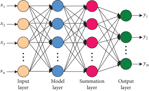
GRNN is a nonlinear regression model based on neural networks. The model maps input data to high-dimensional space through radial basis functions and then convert the output of the hidden layer into the final prediction result through linear combination. The GRNN model has good nonlinear approximation ability and generalization ability and is commonly used in fields such as regression analysis and time series prediction. Its structure is illustrated in Figure 1.

Details are in the caption following the image — **Figure 1**
Open in figure viewer PowerPoint

The model structure of GRNN.

2.1.1. Input Layer

The main function of the input layer refers to receiving input data, and the number of input neurons should be identical to the dimension of the input data.

2.1.2. Model Layer

The number of neurons in the model layer is identical to the number of input data n. The model layer maps input data to the high-dimensional space through the radial basis function to extract the nonlinear characteristics of the data. The function of the radial basis function is to map the input data to the high-dimensional space, making it easier to be separated by the linear classifier. Usually, Gaussian function serves as the radial basis function, as expressed in the following equation [20]:

(1)

where x_i denotes the learning sample of the i-th neuron and σ represents the smoothing parameter.

2.1.3. Summation Layer

A total of two summation methods exist in the summation layer. One is the arithmetic summation of the output of all neurons in the model layer, as expressed in Eq. (2). The other is to conduct the weighted summation of all the neurons in the model layer. The connection weight between the i-th neuron in the mode layer and the j-th neuron in the summation layer is expressed as ω_ij, as written in Eq. (3) [21].

(2)

(3)

2.1.4. Output Layer

The number of neurons in the output layer is identical to the dimension of the input data. The ratio of the summation methods between the two parts of the sum layer is the output of the output layer, as expressed in

(4)

2.2. PSO Algorithm

Particle swarm optimization (PSO) refers to an optimization algorithm based on swarm intelligence, which simulates the behavior of biological groups (e.g., birds or fish) and searches for the optimal solution through continuous iteration [22–24]. The basic idea of PSO algorithm refers to transforming the optimization problem into a search problem in multidimensional space and treating the respective solution as a particle. By continuously updating the position and velocity of particles, it moves towards the direction of the global optimal solution. PSO algorithm has the advantages of strong global search ability, fast convergence speed, and easy implementation, making it suitable for various optimization problems.

The key of PSO algorithm refers to how to update the velocity and position of particles. In general, the velocity and position update equations of particles are expressed as

(5)

(6)

where v_ij(t) represents the velocity of the i-th particle in the j-th dimension, x_ij(t) expresses the position of the i-th particle in the j-th dimension, c₁ and c₂ are acceleration coefficients, r₁(t) and r₂(t) are random numbers, p_ij(t) denotes the optimal position in the history of the i-th particle, and g_ij(t) represents the globally optimal position.

2.3. PSO-GRNN Model

In the conventional GRNN model, the center point and width parameters of the radial basis function are often randomly selected. Meanwhile, the smooth factor in the GRNN model may fall into the local optimal problem, which will lead to the prediction accuracy and generalization ability of the GRNN model cannot achieve the expected results. The PSO-GRNN prediction model is proposed in this study to solve the above-mentioned problems, which uses the PSO algorithm to optimize the GRNN model. The algorithm process is shown in Figure 2, and the specific steps are as follows:

(1)
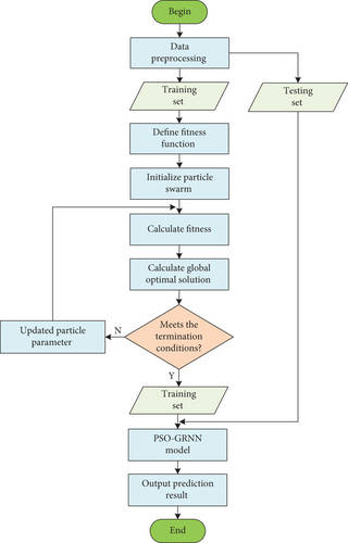
Define fitness function: the fitness function is used to evaluate the fitness of each particle, that is, the prediction accuracy of the model. In GRNN model, the fitness function can be defined as the reciprocal of training error ε (1/ε). The larger fitness function indicates the higher prediction accuracy of the model
(2)
Initialize particle swarm: initialize the position and velocity of the particle swarm, where position represents the center point and width parameters of the radial basis function and velocity denotes the movement direction and velocity of each particle in the search space
(3)
Calculate fitness: calculate the fitness of each particle according to the current position, i.e., the value of the objective function
(4)
Update the global optimal solution: update the global optimal solution in accordance with the current fitness to determine the optimal center point and width parameters of the radial basis function
(5)
Update particle velocity and position: update the particle velocity and position according to the current position and the global optimal solution, causing particles to move towards the direction of the global optimal solution
(6)
Train GRNN model: employ the searched optimal center point and width parameters, with the aim of training the GRNN model and building the final prediction model

2.4. Model Evaluation

In order to verify the predictive advantage of the PSO-GRNN model, four error metrics were used to evaluate the performance of the model which include mean absolute percent error (MAPE) [25], root mean square error (RMSE), R², and NSE. When the MAPE and RMSE values are smaller, it indicates that the predicted values of the model are closer to the true values, and the accuracy and stability of the model are better. However, the closer the values of R² and NSE are to 1, the better the regression effect. The calculation formulas of MAPE, RMSE, R², and NSE are

(7)

(8)

(9)

(10)

where x_i is the measured value of the model, y_i represents the predicted value of the model,

denotes the average value of the measured value,

is the average value of the predicted value, and n is the number of the test samples.

3. Case Analysis

3.1. Project Overview

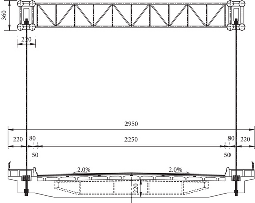
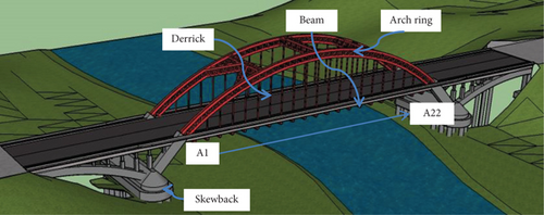
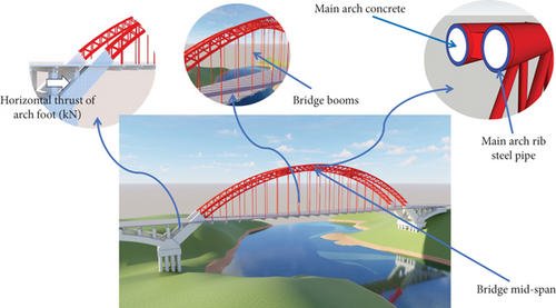
The Qiuhuli Bridge is located in Jiujiang City, Jiangxi Province, China. Its upper structure adopts flying-swallow-typed tied arch structure, with a span arrangement of 45 + 160 + 45 m. The overall layout is presented in Figure 3. A combination of rigid arch and flexible tie rods, with four arch rings Φ 800 mm steel pipes, forms a spatial truss structure, with each steel pipe connected with a transverse steel truss, and the steel pipes are filled with concrete. The height of the arch rib of the main span is 3.6 m, the width of the arch rib reaches 2.2 m, the rise span ratio is set to 1/4, the design alignment of the main arch axis is catenary, and the arch axis coefficient is 1.5. The rise span ratio of the eastern side arch is set to 1/10, the arch axis is catenary, and the arch axis coefficient reaches 1.5. The rise span ratio of the western side arch is 1/9.544, the arch axis is catenary, and the arch axis coefficient is 1.5. The total width of the main bridge reaches 29.5 m, and the bridge deck system adopts π-shaped reinforced concrete prefabricated beams with plate-type rubber bearings. Figure 4 presents the standard cross section of the main bridge.

There are a total of 22 pairs of suspenders in the whole bridge, numbered from left to right as A1 to A22. The suspenders are made of factory produced whole bundle extruded steel strands, with models 15-37. The steel strands are coated with anticorrosion grease, protected by a single HDPE sheath. Moreover, the whole bundle is wrapped with high-strength polyester and then wrapped with HDPE sheath to prevent corrosion of the suspenders. The tied rod pertains to the type of 15-55, which is fully corrosion-resistant, interchangeable, and adjustable. It is anchored at the two ends of the arch ribs on both sides at the arch foot. The respective arch foot comprises six groups of tie rods, each with 55 steel strands. The tie rods are arranged longitudinally in a curved shape. The bridge deck adopts prefabricated trough-shaped plates. The substructure adopts bored pile foundation and rectangular abutment.

Based on Midas/Civil 2020 finite element software, this study establishes a spatial finite element model for the structure analysis of Qiuhuli tied arch bridge. According to the stress characteristics of different components in tied arch bridge, two types of elements are mainly used to achieve, beam element and truss element, in which the suspenders and tie rods are simulated by truss element, and the main arch and its transverse connection, cross tie beam, and substructure are simulated by beam element. The spatial finite element model of the Qiuhuli tied arch bridge consists of 1558 nodes and 2114 elements, including 1400 beam elements and 714 truss elements, which is shown in Figure 5.

3.2. Predictive Analysis Using Horizontal Thrust of Arch Foot and Bulk Weight of Main Beam as Input Variables

During the construction process of filling core concrete to the arch ribs of concrete-filled steel tube arch bridge, there may be differences between the configured concrete and the design values. Secondly, there may be insufficient filling, gaps in the steel pipes, and other reasons. The above-mentioned factors can cause changes in the bulk weight of main arch ring, which can affect the arch rib line shape and stress, as well as the stress of tie beam and the horizontal thrust of arch foot. The design bulk weight of core concrete of the Qiuhuli Bridge is 25 kN/m³. To verify the feasibility and reliability of the improved PSO-GRNN model prediction, this study plans to use the horizontal thrust of arch foot and the bulk weight of main beam as the input variables, to predict the stress values of the upper and lower edges of core concrete and steel pipes at arch foot and mid span arch rib, as well as the displacement of mid span values, which is shown in Figure 6.

The change model of the horizontal thrust of arch foot and the bulk weight of main beam is built using Midas/Civil 2020 finite element software. The stress of main arch rib steel pipe, the stress of main arch concrete, and the displacement of mid span are determined, and the sample data corresponding to the parameter variations in the horizontal thrust of arch foot and the bulk weight of main beam are obtained (Table 1). To be specific, the sample data numbered 1 to 14 pertain to training data, and the sample data numbered 15 to 17 belong to testing data.

Table 1. The corresponding sample data table of horizontal thrust and bulk weight changes.

Sample number	Horizontal thrust of arch foot (kN)	Bulk weight of main beam (kN/m³)	Stress of main arch rib steel pipe (MPa)				Stress of main arch concrete (MPa)				Displacement of mid span (mm)
Sample number	F	γ	σ_1s	σ_1x	σ_2s	σ_2x	σ_1s	σ_1x	σ_2s	σ_2x	Δ
Training sample
1	5070	25	0.934	0.766	0.025	0.039	0.891	0.808	0.000	0.010	46.292
2	5016	25.25	0.938	0.769	0.027	0.041	0.895	0.810	0.001	0.012	46.441
3	4971	25.50	0.942	0.773	0.029	0.043	0.899	0.814	0.002	0.014	46.613
4	4917	25.75	0.946	0.777	0.029	0.043	0.903	0.818	0.002	0.014	46.688
5	4862	26.00	0.950	0.781	0.031	0.045	0.907	0.822	0.004	0.016	46.921
6	4808	26.25	0.953	0.785	0.033	0.047	0.911	0.826	0.006	0.017	47.082
7	4754	26.50	0.959	0.789	0.033	0.048	0.915	0.829	0.006	0.017	47.357
8	4700	26.75	0.963	0.793	0.035	0.048	0.919	0.833	0.008	0.019	47.594
9	4645	27.00	0.967	0.797	0.037	0.050	0.922	0.837	0.008	0.021	47.675
10	4592	27.25	0.971	0.798	0.027	0.056	0.926	0.841	0.010	0.021	47.912
11	4554	27.50	0.975	0.802	0.039	0.054	0.930	0.845	0.012	0.023	48.047
12	4501	27.75	0.979	0.806	0.041	0.054	0.934	0.849	0.012	0.025	48.206
13	4446	28.00	0.983	0.810	0.041	0.056	0.938	0.853	0.014	0.027	48.365
14	4393	28.25	0.986	0.814	0.043	0.058	0.942	0.857	0.014	0.027	48.524
Testing sample
15	4339	28.50	0.990	0.818	0.045	0.060	0.946	0.860	0.016	0.029	48.683
16	4285	28.75	0.994	0.822	0.045	0.060	0.950	0.864	0.017	0.031	48.842
17	4232	29.00	1.000	0.826	0.047	0.062	0.955	0.868	0.017	0.031	49.001

In Table 1, σ_1s expresses the stress at the upper edge of arch foot, σ_1x denotes the stress at the lower edge of arch foot, σ_2s is the stress at the upper edge of mid span arch rib, and σ_2x represents the stress at the lower edge of mid span arch rib.

3.2.1. Data Preprocessing

To improve the recognition accuracy of the PSO-GRNN prediction model, it is necessary to normalize the input data. In this study, Z-score normalization is used to scale the data. Z-score normalization is a data normalization method based on standard deviation, also known as standardization. This method converts data into data with standard normal distribution by converting values with different mean values and standard deviations to values with the same mean values and standard deviations, as shown in

(11)

where z denotes the normalized value, x is the original data value, μ is the average value of the original data, and σ is the standard deviation of the original data. Through Z-score normalization, the average value of the data becomes 0 and the standard deviation is 1.

3.2.2. Model Training and Prediction

As depicted in Table 1, when the horizontal thrust of arch foot and the bulk weight of main beam vary, the stress of main arch rib steel pipe, the stress of main arch concrete, and the displacement of mid span vary notably. After the training sample data are normalized and the sample data are tested, a prediction model is built using MATLAB. The normalized training sample data is adopted to complete the prediction model training, and then, the testing sample data is substituted into the prediction model. The output data of the testing sample serves as the prediction result and compared with the real value. The BP neural network, the GRNN neural network, and the PSO-GRNN method are employed, respectively, to further compare the prediction performance of the PSO-GRNN model. The horizontal thrust of arch foot and the bulk weight of main beam serve as the input variables, and the stress at the lower edge of main arch concrete span, the stress at the lower edge of main arch rib steel pipe span, and the displacement of mid span serve as the output variables to establish the model for prediction. The prediction results are presented in Figures 7, 8, and 9.

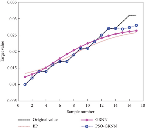
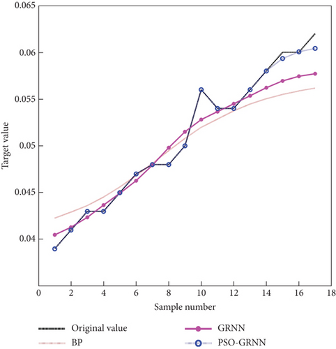
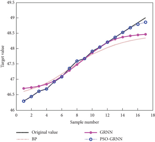
As depicted in Figures 7, 8, and 9, compared with the BP model and the GRNN model, the PSO-GRNN model is capable of well predicting all three variables, such that prediction errors can be significantly reduced. Table 2 lists the prediction errors and average accuracy of the stress at the lower edge of main arch concrete span, the stress at the lower edge of main arch rib steel pipe span, and the displacement of mid span obtained from three prediction models. As revealed by the above-mentioned result, the average prediction accuracy of the PSO-GRNN model reaches 94.949%, 97.274%, and 99.914%, respectively; 10.607%, 5.500%, and 0.976% higher than that of the BP model; and 6.410%, 2.200%, and 0.623% higher than that of the GRNN model. On that basis, the PSO-GRNN model exhibits higher prediction accuracy.

Table 2. Prediction error and average accuracy of three models under horizontal thrust of arch foot and bulk weight of main beam.

Category	Stress at the lower edge of main arch concrete span			Stress at the lower edge of main arch rib steel pipe span			Displacement of mid span
Category	BP	GRNN	PSO-GRNN	BP	GRNN	PSO-GRNN	BP	GRNN	PSO-GRNN
Error of 15	0.0038	0.0023	0.0014	0.0047	0.0026	0.0012	0.4033	0.2091	-0.0170
Error of 16	0.0054	0.0041	0.0020	0.0043	0.0023	0.0009	0.5154	0.3421	0.0068
Error of 17	0.0051	0.0041	0.0012	0.0060	0.0041	0.0029	0.6377	0.4886	0.1015
Average accuracy	84.342%	88.539%	94.949%	91.774%	95.074%	97.274%	98.938%	99.291%	99.914%

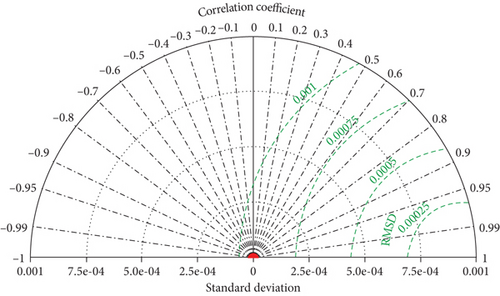
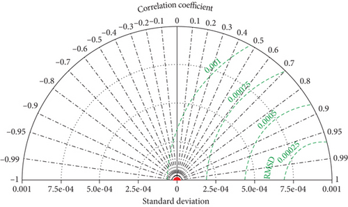
In order to further compare the prediction performance of the BP model, GRNN model, and PSO-GRNN model, four error indicators, MAPE, RMSE, R², and NSE, were used to evaluate the prediction performance of the model. The results are shown in Table 3, and the Taylor diagram of the PSO-GRNN model predicted results is shown in Figure 10 [26, 27]. From the results, it can be seen that the PSO-GRNN model has the highest fitting accuracy, with R² and NSE values close to 1, and MAPE and RMSE values are very small. Thus, the performance of the PSO-GRNN model is better than that of the BP model and GRNN model.

Table 3. Comparison of prediction performance under horizontal thrust of arch foot and bulk weight of main beam.

Category	Stress at the lower edge of main arch concrete span			Stress at the lower edge of main arch rib steel pipe span			Displacement of mid span
Category	BP	GRNN	PSO-GRNN	BP	GRNN	PSO-GRNN	BP	GRNN	PSO-GRNN
MAPE	0.264	0.183	0.125	0.168	0.138	0.113	0.154	0.068	0.035
RMSE	2.025	1.023	0.017	3.023	2.121	1.018	4.135	3.097	0.038
R²	0.505	0.627	0.915	0.495	0.541	0.843	0.454	0.716	0.938
NSE	0.871	0.889	0.989	0.871	0.889	0.918	0.823	0.908	0.985

3.3. Predictive Analysis Using Horizontal Thrust of Arch Foot and Tension of Tied Rod as Input Variables

The existing application of prestressed structures turns out to be progressively widespread, and the damage and destruction arising from the relaxation of prestressed steel bars are increasing. The tie rods of the Qiuhuli Bridge are anchored at the arch foot at both ends of the side arch ribs. The respective arch foot comprises six groups of tie rods, each with 55 steel strands. The tie rods are arranged longitudinally in a curved shape. The tension of the tie rod can be reduced due to the loss of prestress and anchor deformation. In this section, the horizontal thrust of arch foot and the tension of tie rod serve as the input variables, and the stress of main arch rib steel pipe, the stress of main arch concrete, and the displacement of mid span serve as the output variables. Analysis and calculation are conducted using Midas/Civil 2020 finite element software, and the sample data are acquired (Table 4). The sample data numbered 1 to 10 refer to training data, and the sample data numbered 11 to 13 pertain to testing data.

Table 4. The prediction sample data table of horizontal thrust of arch foot and tension of tied rod.

Sample number	Horizontal thrust of arch foot (kN)	Tension of tied rod (kN)	Stress of main arch rib steel pipe (MPa)				Stress of main arch concrete (MPa)				Displacement of mid span (mm)
Sample number	F	F	σ_1s	σ_1x	σ_2s	σ_2x	σ_1s	σ_1x	σ_2s	σ_2x	Δ
Training sample
1	5294.8	300	0.996	0.819	0.031	0.045	0.951	0.862	0.002	0.014	46.37
2	5575.6	297	0.998	0.819	0.033	0.047	0.951	0.862	0.004	0.016	46.30
3	5846.3	294	0.998	0.819	0.033	0.047	0.953	0.862	0.004	0.016	46.22
4	6127.14	292	0.998	0.819	0.033	0.047	0.953	0.862	0.004	0.016	46.15
5	6407.9	289	0.998	0.819	0.033	0.049	0.953	0.862	0.004	0.018	46.07
6	6678.6	286	0.998	0.819	0.035	0.049	0.953	0.864	0.006	0.018	45.99
7	6949.6	283	1.000	0.821	0.035	0.049	0.953	0.864	0.006	0.018	45.92
8	7230.1	281	1.000	0.821	0.035	0.051	0.955	0.864	0.006	0.021	45.84
9	7510.9	278	1.000	0.821	0.035	0.051	0.955	0.864	0.006	0.021	45.77
10	5294.8	275	0.996	0.819	0.031	0.045	0.951	0.862	0.002	0.014	46.37
Testing sample
11	5010.3	272	0.996	0.819	0.031	0.045	0.949	0.862	0.002	0.014	46.12
12	4963.3	269	0.994	0.799	0.029	0.043	0.949	0.862	0.002	0.014	46.00
13	4756.3	265	0.994	0.799	0.029	0.043	0.947	0.860	0.001	0.012	45.95

In Table 4, σ_1s expresses the stress at the upper edge of arch foot, σ_1x denotes the stress at the lower edge of arch foot, σ_2s is the stress at the upper edge of mid span arch rib, and σ_2x represents the stress at the lower edge of mid span arch rib.

3.3.1. Data Preprocessing

To facilitate neural network identification, it is necessary to normalize the input data. The processing of data normalization in this part is identical to that in Section 3.2.1, so it will not be repeated here.

3.3.2. Model Training and Prediction

According to Table 4, when the horizontal thrust of arch foot and the tension of tied rod change, the stress of main arch rib steel pipe, the stress of main arch concrete, and the displacement of mid span change significantly. After normalizing the training sample data and testing sample data, a prediction model is built using MATLAB. The normalized training sample data is used to complete the prediction model training, and then, the testing sample data is substituted into the prediction model. The output data of the testing sample serves as the prediction result and is compared with the real value. To further compare the prediction performance of the PSO-GRNN model, three methods are used: the BP model, the GRNN model, and the PSO-GRNN model. The horizontal thrust of arch foot and the tension of tied rod serve as the input variables, and the stress at the lower edge of main arch concrete span, the stress at the lower edge of main arch rib steel pipe span, and the displacement of mid span serve as the output variables to establish the model for prediction. The prediction results are shown in Figures 11, 12, and 13.

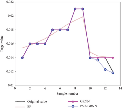
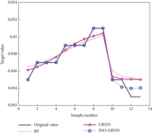
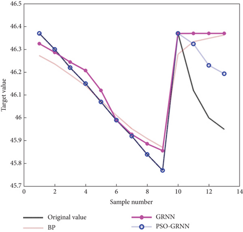
As depicted in Figures 10, 11, and 12, after using the horizontal thrust of arch foot and the tension of tie rod as input variables, compared with the BP model and GRNN model, the PSO-GRNN model can still make a good prediction of the three variables, greatly reducing the prediction error. Table 5 presents the prediction errors and average accuracy of the stress at the lower edge of main arch concrete span, the stress at the lower edge of main arch rib steel pipe span, and the displacement of mid span of the three prediction models. It can be seen that the average prediction accuracy of the PSO-GRNN model is 96.706%, 98.531%, and 99.634%, respectively, which is 1.980%, 1.706%, and 0.340% higher than that of the BP model. Compared with the average accuracy of the GRNN model, it is improved by 2.262%, 1.632%, and 0.387%, suggesting that PSO-GRNN model has higher prediction accuracy.

Table 5. Prediction error and average accuracy of three models under horizontal thrust of arch foot and tension of tied rod.

Category	Stress at the lower edge of main arch concrete span			Stress at the lower edge of main arch rib steel pipe span			Displacement of mid span
Category	BP	GRNN	PSO-GRNN	BP	GRNN	PSO-GRNN	BP	GRNN	PSO-GRNN
Error of 11	-0.0001	0.0000	0.0002	-0.0001	0.0000	0.0001	-0.2135	-0.2500	-0.1732
Error of 12	-0.0001	0.0000	0.0006	-0.0020	-0.0020	-0.0014	-0.3483	-0.3700	-0.1628
Error of 13	-0.0020	-0.0020	-0.0005	-0.0020	-0.0020	-0.0004	-0.4125	-0.4200	-0.1696
Average accuracy	94.726%	94.444%	96.706%	96.825%	96.899%	98.531%	99.294%	99.247%	99.634%

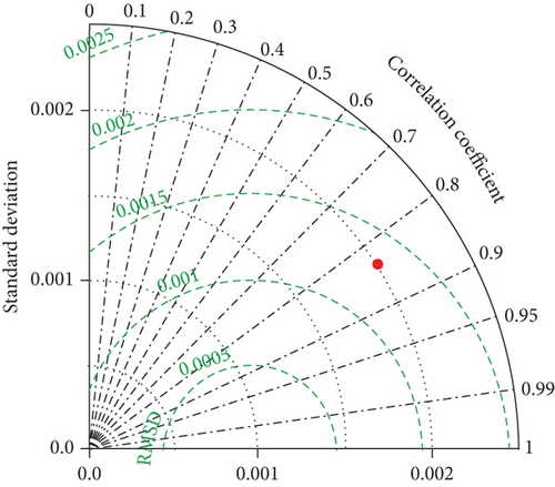
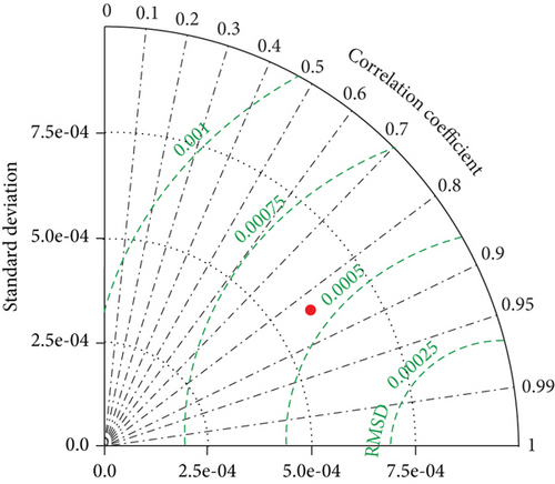
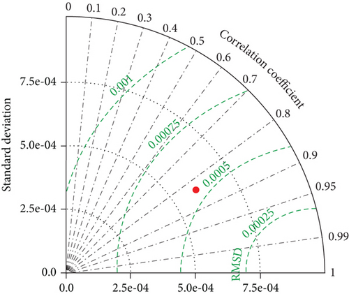
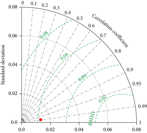
Similarly, the prediction performance of the three models was evaluated using four error indicators: MAPE, RMSE, R², and NSE. The results are shown in Table 6, and the Taylor diagram of the PSO-GRNN model predicted results is shown in Figure 14. From the results, it can be seen that the PSO-GRNN model has the highest fitting accuracy, with R² and NSE values close to 1, and MAPE and RMSE values are very small. Thus, the performance of the PSO-GRNN model is better than that of the BP model and GRNN model.

Table 6. Comparison of prediction performance under horizontal thrust of arch foot and tension of tied rod.

Category	Stress at the lower edge of main arch concrete span			Stress at the lower edge of main arch rib steel pipe span			Displacement of mid span
Category	BP	GRNN	PSO-GRNN	BP	GRNN	PSO-GRNN	BP	GRNN	PSO-GRNN
MAPE	0.236	0.167	0.128	0.184	0.152	0.118	0.216	0.173	0.077
RMSE	6.088	4.028	1.013	3.874	1.548	0.427	3.151	2.143	1.031
R²	0.519	0.674	0.924	0.581	0.657	0.927	0.528	0.712	0.882
NSE	0.848	0.886	0.977	0.871	0.912	0.975	0.659	0.731	0.901

4. Conclusion

Through the application of the PSO-GRNN model in the health monitoring technology of flying-swallow-typed tied arch bridge, the conclusions obtained are as follows:

(1)
In the construction control of large-span concrete-filled steel tube tied arch bridge, finite element analysis software is used to establish a calculation model, which can analyze the stress situation of the bridge. This article uses Midas/Civil 2020 software for finite element modeling of bridges and constructs a prediction model based on PSO-GRNN algorithm to predict the partial stress situation of bridges, simplifying the number of finite element analysis models and having high practical value
(2)
By using the PSO algorithm to optimize the GRNN model, a PSO-GRNN prediction model is proposed. Z-score normalization is used to standardize the data, solving the problem of parameters falling into local optima in conventional GRNN models and improving the prediction accuracy of the PSO-GRNN model
(3)
The average prediction accuracy of the PSO-GRNN model is higher than that of the BP model and GRNN model, and the prediction effect is better. By comparing MAPE, RMSE, R², and NSE, it is shown that the PSO-GRNN model has the highest fitting accuracy. This indicates that the PSO-GRNN model proposed in this study is effective. The result of this study is consistent with the accuracy of Wang et al. [28] in predicting the health status of lithium-ion batteries using the PSO-GRNN algorithm, which further indicates that PSO-GRNN algorithm has excellent prediction ability
(4)
The PSO-GRNN prediction model constructed in this article has a high fitting accuracy, but due to the small amount of training and testing samples, the number of training and testing samples will be further increased in the future to further improve the application of the PSO-GRNN prediction model. At the same time, we will continue to research and explore more optimization algorithms to improve the performance of prediction models

Conflicts of Interest

The authors declare no conflicts of interest regarding this article.

Authors’ Contributions

All the authors have accepted responsibility for the entire content of this submitted manuscript as an approved submission.

Acknowledgments

This research was funded by Key Problems in Science and Technology of Henan Provincial (222102320040).

Open Research

Data Availability

The data used to support the findings of this study are included within the article.

References

1 Li Z., Zhou Y., Lan T., Dong Z., and Xiong Meng M., Performance evaluation of prestressed concrete containment sturctuce based on finite element model updating, Industrial Construction. (2022) 52, no. 10, 84–88+77.
Google Scholar
2 Fu L., Ma W., Gao P., Zhou J., Zhang J., and Zhao Y., Modification of bridge structure finite element model based on RSM-WOA, China Sciencepaper. (2021) 16, no. 8, 875–882.
Google Scholar
3 Tian S., Xia F., and Wang L., Review of the research on correction methods of bridge finite element model, Engineering and Technological Research. (2022) 7, no. 7, 190–192.
Google Scholar
4 Gu J., Xiang C., Tao F., Huang M., Jia W., and Wang F., Ridge structure model updating method based on deep learning and IHPO, Journal of Guangxi University (Natural Science Edition). (2022) 47, no. 5, 1147–1159.
Google Scholar
5 Ardani S., Azam S. E., and Linzell D. G., Bridge health monitoring using proper orthogonal decomposition and transfer learning, Applied Sciences. (2023) 13, no. 3, https://doi.org/10.3390/app13031935.
10.3390/app13031935
Google Scholar
6 Singh P., Mittal S., and Sadhu A., Recent advancements and future trends in indirect bridge health monitoring, Practice Periodical on Structural Design and Construction. (2023) 28, no. 1.
10.1061/PPSCFX.SCENG-1259
Web of Science® Google Scholar
7 Ghahremani B., Enshaeian A., and Rizzo P., Bridge health monitoring using strain data and high-fidelity finite element analysis, Sensors. (2022) 22, no. 14, https://doi.org/10.3390/s22145172, 35890852.
10.3390/s22145172
PubMed Web of Science® Google Scholar
8 Xu Y. and Qiu J., Internet-based centralized remote real-time long-span bridge health monitoring system, Journal of Computational Methods in Sciences and Engineering. (2023) 23, no. 2, 781–797, https://doi.org/10.3233/JCM-226588.
10.3233/JCM-226588
Web of Science® Google Scholar
9 Zhang J., Zhao X., Gao Y., Guo W., and Zhai Y., Shear strength prediction and failure mode identification of beam–column joints using BPNN, RBFNN, and GRNN, Arabian Journal for Science and Engineering. (2022) 48, no. 4, 4421–4437.
10.1007/s13369-022-07001-2
Web of Science® Google Scholar
10 Zhao F., Chen C., Han B., and Qian F., BP-GRNN model for deformation prediction of diaphragm wall based on multi-source data, International Journal of Earth Sciences and Engineering. (2016) 9, no. 3, 888–893.
Google Scholar
11 Ning Y., Cui X., and Cui J., Deformation prediction of open-pit mine slope based on ABC-GRNN combined model, Coal Geology & Exploration. (2023) 51, no. 3, 65–72.
Google Scholar
12 Ekrani S. M., Ganjehzadeh S., and Esfahani J. A., Multi-objective optimization of a tubular heat exchanger enhanced with delta winglet vortex generator and nanofluid using a hybrid CFD-SVR method, International Journal of Thermal Sciences. (2023) 186, article 108141, https://doi.org/10.1016/j.ijthermalsci.2023.108141.
10.1016/j.ijthermalsci.2023.108141
Web of Science® Google Scholar
13 Samanataray S. and Sahoo A., A comparative study on prediction of monthly streamflow using hybrid ANFIS-PSO approaches, KSCE Journal of Civil Engineering. (2021) 25, no. 10, 4032–4043, https://doi.org/10.1007/s12205-021-2223-y.
10.1007/s12205-021-2223-y
Web of Science® Google Scholar
14 Chaudhury S., Samantaray S., Sahoo A., Bhagat B., Biswakalyani C., and Satapathy D. P., V. Bhateja, J. Tang, S. C. Satapathy, P. Peer, and R. Das, Hybrid ANFIS-PSO model for monthly precipitation forecasting, Evolution in Computational Intelligence. Smart Innovation, Systems and Technologies, vol. 267, 2022, Springer, Singapore, https://doi.org/10.1007/978-981-16-6616-2_33.
10.1007/978-981-16-6616-2_33
Google Scholar
15 Samantaray S., Sah M. K., Chalan M. M., Sahoo A., and Mohanta N. R., V. Bhateja, L. Khin Wee, J. C. W. Lin, S. C. Satapathy, and T. M. Rajesh, Data engineering and intelligent computing, Lecture Notes in Networks and Systems, vol 446, 2022, Springer, Singapore, https://doi.org/10.1007/978-981-19-1559-8_29.
Google Scholar
16 Li Q., Yang Y., Yan K., and Chen H., Study on factors affecting fatigue performance of suspender of flying swallow steel box tied arch bridge, Technology of Highway and Transport. (2019) 35, no. 2, 92–97+109.
Google Scholar
17 Liu L. and Wang N., Calculation and analysis for large span flying swallow type of tied arch bridge, Highways & Transportation in Inner Mongolia. (2016) 5, 25–28.
Google Scholar
18 Li H., Shen Z., and Zhang W., Inversion of permeability coefficient for concrete face rockfill dam based on PSO-GRNN and its application, Water Resources and Power. (2023) 41, no. 5, 67–70+80.
Google Scholar
19 Andrade C., Z scores, standard scores, and composite test scores explained, Indian Journal of Psychological Medicine. (2021) 43, no. 6, 555–557, https://doi.org/10.1177/02537176211046525, 35210687.
10.1177/02537176211046525
PubMed Google Scholar
20 Richards D. and Zheng Q., A reflection formula for the Gaussian hypergeometric function of matrix argument, Journal of Mathematical Analysis and Applications. (2024) 531, no. 2, article 127862 Part 2, https://doi.org/10.1016/j.jmaa.2023.127862.
10.1016/j.jmaa.2023.127862
Web of Science® Google Scholar
21 Zhou C., Wang C., Sun Y., and Yao W., Weighted sum synchronization of memristive coupled neural networks, Neurocomputing. (2020) 403, 211–223, https://doi.org/10.1016/j.neucom.2020.04.087.
10.1016/j.neucom.2020.04.087
Web of Science® Google Scholar
22 Weng Z., He F., and Hu Z., Study on correction method of tunnel kiln simulation model based on PSO-BP algorithm, Machine Building & Automation. (2023) 52, no. 1, 105–109.
Google Scholar
23 Tang Z. and Xu J., PSO optimizing bridge deformation prediction for LSTM time series, Beijing Surveying and Mapping. (2023) 37, no. 1, 115–119.
Google Scholar
24 Bao L., Yan J., Wang X., Bai Z., and Yu L., Research on optimal layout of continuous beam bridge health monitoring sensor based on improved PSO algorithm, Journal of Shenyang Jianzhu University Natural Science. (2022) 38, no. 6, 1072–1079.
Google Scholar
25 Bayram S. and Çıtakoğlu H., Modeling monthly reference evapotranspiration process in Turkey: application of machine learning methods, Environmental Monitoring and Assessment. (2023) 195, no. 1, https://doi.org/10.1007/s10661-022-10662-z, 36329360.
10.1007/s10661-022-10662-z
PubMed Web of Science® Google Scholar
26 Özbayrak A., Ali M. K., and Çıtakoğlu H., Buckling load estimation using multiple linear regression analysis and multigene genetic programming method in cantilever beams with transverse stiffeners, Arabian Journal for Science and Engineering. (2023) 48, no. 4, 5347–5370, https://doi.org/10.1007/s13369-022-07445-6.
10.1007/s13369-022-07445-6
Web of Science® Google Scholar
27 Zouzou Y. and Citakoglu H., General and regional cross-station assessment of machine learning models for estimating reference evapotranspiration, Acta Geophysica. (2023) 71, no. 2, 927–947, https://doi.org/10.1007/s11600-022-00939-9.
10.1007/s11600-022-00939-9
Web of Science® Google Scholar
28 Wang J. X., Zhu L. Q., and Dai H. D., An efficient state-of-health estimation method for lithium-ion batteries based on feature-importance ranking strategy and PSO-GRNN algorithm, Journal of Energy Storage. (2023) 72, article 108638, no. Part D, https://doi.org/10.1016/j.est.2023.108638.
10.1016/j.est.2023.108638
Web of Science® Google Scholar

All articles

Research on Health Monitoring of Flying-Swallow-Typed Tied Arch Bridge Based on PSO-GRNN Algorithm

Abstract

1. Introduction

2. Prediction Model Based on PSO-GRNN Algorithm