Modeling the Effects of Ehrlichia chaffeensis and Movement on Dogs
Abstract
Ehrlichia chaffeensis is a tick-borne infectious disease transmitted by Amblyomma americanum tick. This infectious disease was discovered in the 1970s when military dogs were returning from the Vietnam War. The disease was found to be extremely severe in German Shepherds, Doberman Pinschers, Belgium Malinois, and Siberian Huskies. In this study, we developed a mathematical model for dogs and ticks infected with Ehrlichia chaffeensis with the aim of understanding the impact of movement on dogs as they move from one location to another. This could be a dog taken on a walk in an urban area or on a hike in the mountains. We carried out a global sensitivity analysis with and without movement between three locations using as response functions the sum of acutely and chronically infected ticks and the sum of infected ticks in all life stages. The parameters with the most significant impact on the response functions are dogs disease progression rate, dogs chronic infection progression rate, dogs recovery rate, dogs natural death rate, acutely and chronically infected dogs disease-induced death rate, dogs birth rate, eggs maturation rates, tick biting rate, dogs and ticks transmission probabilities, ticks death rate, and the location carrying capacity. Our simulation results show that infection in dogs and ticks are localized in the absence of movement and spreads between locations with highest infection in locations with the highest rate movement. Also, the effect of the control measures which reduces infection trickles to other locations (trickling effect) when controls are implemented in a single location. The trickling effect is strongest when control is implemented in a location with the highest movement rate into it.
1. Introduction
Ehrlichia chaffeensis is a tick-borne infectious disease that lives within white blood cells. The disease was first recognized in Africa during the 1930s. This infectious disease originated in the United States in the 1970s, when military dogs were returning from the Vietnam War. It is estimated that 200–250 million dogs died from this disease in Vietnam. Due to the high infection rates of dogs a majority of the war dogs were left behind in Vietnam [1]. They found this disease to be extremely severe in German Shepherds, Doberman Pinschers, Belgium Malinois, and Siberian Huskies. This disease can also be referred to as tracker dog disease and tropical canine pancytopenia [2].
One primary vector of Ehrlichia chaffeensis is the Amblyomma americanum tick. It is mostly found in south-central and eastern United States [3]. It is also referred to as the Lone Star tick. The tick goes through four different life stages. These life stages are egg, larvae, nymph, and adult, which typically take two years to complete [4]. The adult ticks are typically the ones that feed on dogs. They are seen active March through August in the Midwest [5]. There is currently no vaccine for dogs in preventing Ehrlichia Chaffeensis. The way of prevention is by preventing ticks on pets and in yards.
There are two stages of infection with Ehrlichia chaffeensis in dogs. The first 2–4 weeks of infection are referred to as the acute stage. During this stage, symptoms include fever, swollen lymph nodes, respiratory distress, weight loss, bleeding disorders, and sometimes neurological disturbances. There is an antibody and PCR test for Ehrlichia chaffeensis in dogs. The antibody test could remain negative during the first week of illness and could remain positive for months to years. There is a rapid antibody test that gives results within minutes or there is an ELISA and IFA antibody test that takes days or weeks for results. The PCR test can provides species-specific results and can take days for results. Dogs are treated for Ehrlichia chaffeensis with a 28-day treatment of doxycycline. After 24–72 hours of initiating treatment the clinical signs should resolve [6]. After 2–4 weeks the dog will recover or progress into the clinical/chronic stage. During the clinical/chronic stage dogs may develop symptoms such as anemia, bleeding episodes, lameness, eye problems, neurological problems, and swollen limbs. The clinical/chronic stage typically leads to death [2]. There is no correlation between the age of dog and the severity of the infection stage [7]. Dogs are capable of being reinfected of Ehrlichia chaffeensis; however, dogs cannot pass the disease on to their offspring.
To prevent dogs from being infected with Ehrlichia chaffeensis, it is advised to use proper tick prevention techniques. This may include collars, monthly topical, or oral preventatives year round. It is not recommended to use human insect repellent on dogs. After dogs have spent time outside it is recommended to thoroughly evaluate them for ticks. Removing a tick right away reduces the risk of disease transmission. To remove a tick, it is recommended to use fine-tipped tweezers and grab the tick closely to the skin’s surface. Then proceed to pull with a steady pressure upwards [6].
The goal of this study is to produce a mathematical model to better understand the transmission of Ehrlichia chaffeensis between dogs and Amblyomma americanum. This model will also be used to better understand the impact of movement on dogs as they move from one location to another. This could be taking a dog on a walk in an urban area or taking a dog on a hike in the mountains. A preprint of this study is already available on bioRxiv [8].
The rest of the paper is organized as follows: in Section 2, we present the Ehrlichia chaffeensis mathematical model for a single location with no movement, the basic qualitative analysis of the model including results of the positivity and boundedness of solutions, the computation of the reproduction number, and global sensitivity analysis. In Section 3, we introduce the Ehrlichia chaffeensis model with movement between different locations. In this section, we also implement a global sensitivity analysis in the absence and presence of movement. Using results from the sensitivity analysis we simulate the model with movement to determine the effect of disease transmission and ticks natural death when the locations are isolated and when they are connected by movement. In Section 4, we discuss and give conclusions of the results obtained from this study, followed by some recommendations to dog owners.
2. Model Formulation
The conceptualized flow diagram of the Ehrlichia chaffeensis transmission in dogs model is shown in Figure 1. The corresponding parameters and variables are described in Table 1.
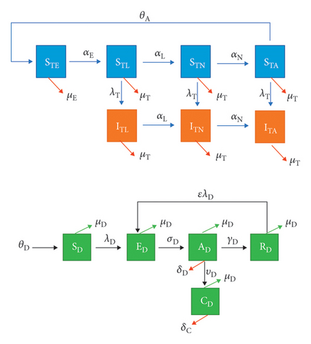
| Variable | Description |
|---|---|
| SD | Population of susceptible dogs |
| ED | Population of exposed dogs |
| AD | Population of acute stage of infection in dogs |
| CD | Population of chronic stage of infection in dogs |
| RD | Population of recovered dogs |
| STE | Susceptible tick eggs |
| STL, STN, STA | Population of susceptible larvae, nymphs, and adult ticks |
| ITE | Infected tick eggs |
| ITL, ITN, ITA | Population of infected larvae, nymphs, and adult ticks |
| Parameter | Description |
| θD | Birth rate of dogs |
| γD | Recovery rate in dogs |
| υD | Acute to chronic disease progression rate in dogs |
| σD | Disease progression rate in dogs |
| ε | Reinfection rate of in dogs |
| αE | Tick eggs to larvae maturation rate |
| αL | Larvae to nymphs maturation rate |
| αN | Nymphs to adult ticks maturation rate |
| θA | Ticks egg laying rate |
| μE | Tick eggs decay rate |
| μL, μN, μA | Larvae, nymphs, adult ticks death rate |
| μD | Natural death rate of dogs |
| δD | Acute infection death rate in dogs |
| δC | Chronic infection death rate in dogs |
| βD | Dog transmission probability |
| ϕT | Tick biting rate |
| βT | Tick transmission probability |
2.1. Analysis of the Model
2.1.1. Basic Qualitative Properties
(1) Positivity and Boundedness of Solutions. For the Ehrlichia chaffeensis model (6) to be epidemiologically meaningful, it is important to prove that all its state variables are non-negative for all time. In other words, solutions of the model system (6) with non-negative initial data will remain non-negative for all time t > 0.
Lemma 1. Let the initial data (0) ≥ 0, where F(t) = (SD(t), ED(t), AD(t), CD(t), RD(t), STE(t), STL(t), ITL(t), STN(t), ITN(t), STA(t), ITA(t)). Then, the solutions F(t) of the Ehrlichia chaffeensis model (6) are non-negative for all t > 0. Furthermore,
The proof of Lemma 1 is given in Appendix A.
Lemma 2. The region is positively-invariant for the model (6) with non-negative initial conditions in .
The prove of Lemma 2 is given in Appendix B.
In the next section, the conditions for the existence and stability of the equilibria of the model (6) are stated.
The expression is the number of secondary infections in dogs. The expressions is the number of secondary infections in ticks from a single infectious dog. Further, using Theorem 2 in [12], the following result is established.
Lemma 3. The disease-free equilibrium (DFE) of the Ehrlichia chaffeensis model (14) is locally asymptotically stable (LAS) if and unstable if .
The basic reproduction number is defined as the average number of new infections that result from one infectious individual (tick or dog) in a population that is fully susceptible [12–14]. The epidemiological significance of Lemma 3 is that Ehrlichia chaffeensis will be eliminated from within a herd if the reproduction number can be brought to (and maintained at) a value less than unity.
2.2. Sensitivity Analysis of Model (14)
In order to determine the contribution of each of the model parameters to key model outputs (such as the number of infected), one can use a sensitivity analysis procedure [22–24]. Results of the sensitivity analysis help to identify the system parameters that are the best to target during an intervention, and also for future surveillance data gathering. We carried out a global sensitivity analysis using Latin Hypercube Sampling (LHS) and partial rank correlation coefficients (PRCC) to assess the impact of parameter uncertainty and the sensitivity of these key model outputs. The LHS method is a stratified sampling technique without replacement this allows for an efficient analysis of parameter variations across simultaneous uncertainty ranges in each parameter [25–28]. On the other hand, PRCC measures the strength of the relationship between the model outcome and the parameters, stating the degree of the effect that each parameter has on the model outcome [25–28].
We start by generating the LHS matrices and assuming all the model parameters are uniformly distributed. We then carry out a total of 1,000 simulations (runs) of the model for the LHS matrix, using the parameter values given in Table 2 (with ranges varying from ±20% of the stated baseline values) and as response functions, the sum of carries and infected. The parameter ranking using PRCC is then implemented following these simulation runs.
| Parameter | Description | Value (1/day) | Reference(s) |
|---|---|---|---|
| θD | Birth rate of dogs | 70,000 | [15] |
| γD | Rate of infected to recovered dogs | 0.04761905 | [2] |
| υD | Rate of acute to chronic infection in dogs | 0.04761905 | [2] |
| σD | Rate of exposed to infected dogs | 0.07142857 | [10] |
| ε | Rate of reinfection in dogs | 0.00444444 | [16] |
| αE | Maturation rate from tick eggs to larvae | 0.02439024 | [17] |
| αL | Maturation rate from tick larvae to nymphs | 0.00273973 | [17] |
| αN | Maturation rate from nymphs to adult ticks | 0.0037037 | [17] |
| θA | Ticks egg laying rate | 6000 eggs | [18] |
| μE | Death rate of tick eggs | 0.008 | [18] |
| μT | Death rate of ticks | 0.003 | [18] |
| μD | Natural death rate of dogs | 0.00027397 | [19] |
| δD | Acute infection death rate in dogs | 0.1735 | Assumed |
| δC | Chronic infection death rate in dogs | 0.347 | [20] |
| βD | Dog transmission probability | 0.152 | [21] |
| ϕT | Tick biting rate | 0.044 | Assumed |
| βT | Tick transmission probability | 0.152 | [21] |
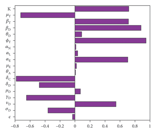
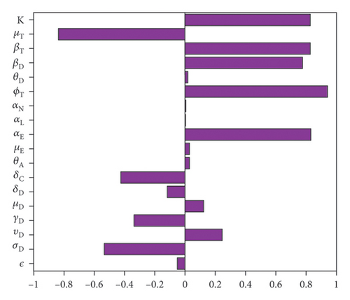
The outcome of the global sensitivity analysis is shown in Figure 2 and given in Table 3. The parameters with substantial effect on the sum of the acutely and chronically infected dogs are those parameters whose sensitivity index have significant p values less than or equal to 0.05. The parameters with the most impacts on (AD + CD), are disease progression rate in dogs (σD), the rate (υD) dogs progress to chronic infection from acute infection, dog recovery rate (γD), the natural death rate of dogs (μD), death rate (δD) of acutely infected dogs, death rate of the chronically infected dogs (δC), birth rate of dogs (θD), the maturation rates eggs to larvae (αE), the tick biting rate (ϕT), the dog transmission probability (βD), the tick transmission probability (βT) and death rate of ticks (μT), and the carrying capacity K. For the sum of infected larvae, nymphs, and adult ticks (ITL + ITN + ITA), the significant parameters are υD, σD, μD, δD, δC, μE, αE, ϕT, θD, βT, and μT.
| Parameters | AD + CD | ITL + ITN + ITA | ||
|---|---|---|---|---|
| PRCC | p value | PRCC | p value | |
| ε | −0.0335 | 0.2938 | −0.0491 | 0.1242 |
| σD | −0.3604 | ≤0.0001 | −0.5323 | ≤0.0001 |
| υD | 0.5466 | ≤0.0001 | 0.2460 | ≤0.0001 |
| γD | −0.6476 | ≤0.0001 | −0.3367 | ≤0.0001 |
| μD | 0.0711 | 0.0258 | 0.1217 | 0.0001 |
| δD | −0.4754 | ≤0.0001 | −0.1163 | 0.0003 |
| δC | −0.7851 | ≤0.0001 | −0.4235 | ≤0.0001 |
| θA | 0.0051 | 0.8728 | 0.0300 | 0.3478 |
| μE | 0.0184 | 0.5642 | 0.0296 | 0.3544 |
| αE | 0.7043 | ≤0.0001 | 0.8301 | ≤0.0001 |
| αL | 0.0364 | 0.2548 | 0.0040 | 0.8991 |
| αN | 0.0117 | 0.7142 | 0.0048 | 0.8815 |
| ϕT | 0.9484 | 0 | 0.9424 | 0 |
| θD | 0.0893 | 0.0051 | 0.0191 | 0.5488 |
| βD | 0.8800 | ≤0.0001 | 0.7770 | ≤0.0001 |
| βT | 0.7142 | ≤0.0001 | 0.8274 | ≤0.0001 |
| μT | −0.7243 | ≤0.0001 | −0.8346 | ≤0.0001 |
| K | 0.7164 | ≤0.0001 | 0.8271 | ≤0.0001 |
The PRCC index values of some of these parameters have positive signs while others have negative signs. The positive signs means that any increase in these parameters will lead to an increase in the response functions (AD + CD, and ITL + ITN + ITA). While the negative signs implies increase in the parameters will lead to a decrease in the response functions. Hence, these parameters would be useful targets during mitigation efforts.
Therefore, control strategies which target those parameters with significant PRCC values will give the greatest impact on the model response functions. For instance, a control that aims for a 10% decrease in the transmission probability in dogs (βD) will lead to 88% reduction in infected dogs (AD + CD) and about 78% reduction in infected ticks (ITL + ITN + ITA). Similarly a 10% decrease in the ticks transmission probability (βT) will lead to 71.4% reduced infection in dogs and about 83% reduced infection in ticks. Also, a 10% deduction in tick biting rate (ϕT) will lead to about 95% reduction in infected dogs, and about 94% reduction in infected ticks. Furthermore, a 10% increase in ticks death rate (μT) will result in about 72.4% reduction in infected dogs and about 83.4% decrease in ticks.
3. Movement Model
3.1. Sensitivity Analysis of Model (27) with Movement
To carry out global sensitivity analysis for the Ehrlichia chaffeensis model (27) with movement, we also use two response functions, the sum of infected dogs and the sum of infected ticks , i = 1, 2, 3. As with the case of model (14) above, we implemented the sensitivity analysis to determine the impact of the model parameters on these two response functions. We implemented the analysis using three different locations and considered two scenarios: (i) when the locations are isolated and (ii) when the locations are connected.
To carry out the sensitivity analysis, we fixed some parameters related to the natural history of the infection in dogs and ticks. We then assume the values of parameters like dog birth rate , the carrying capacity (Ki), dogs and ticks transmission probabilities (, and ), and ticks death rate are location dependent since the different locations might have different climatic conditions or microclimates.
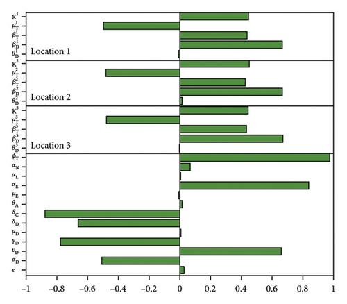
Figure 3 and Table 4 the results of the sensitivity analysis and the p values of the parameters for the case with no movement between the regions. The results show the parameters with the most impact on the sum of infected dogs and the sum of infected larvae, nymphs, and adult ticks . Observe that some parameters have positive PRCC values while others have negative values. Thus, the significant parameters are disease progression rate in dogs (σD), the rate (υD) dogs progress to chronic infection from acute infection, dog recovery rate (γD), the natural death rate of dogs (μD), death rate (δD) of acutely infected dogs, death rate of chronically infected dogs (δC), birth rate of dogs , the maturation rates of eggs to larvae (αE), the tick biting rate (ϕT), the dog transmission probability (βD), the tick transmission probability and death rate of ticks , and the carrying capacity Ki. The PRCC values of parameters , Ki, , , and are relatively the same since there are no movement between the region.
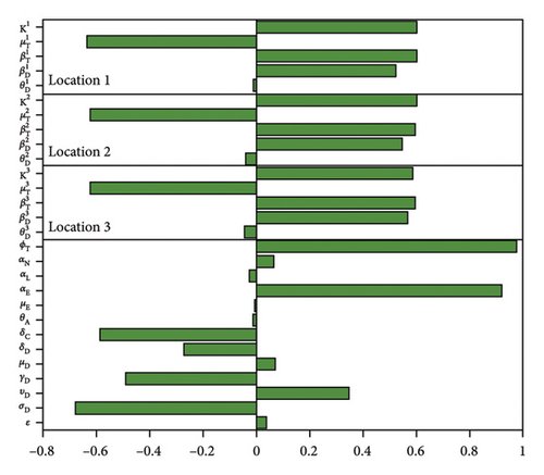
| Parameters | AD + CD | ITL + ITN + ITA | ||
|---|---|---|---|---|
| PRCC | p value | PRCC | p value | |
| ε | 0.0279 | 0.3853 | 0.0378 | 0.2388 |
| σD | −0.5088 | ≤0.0001 | −0.6808 | ≤0.0001 |
| υD | 0.6599 | ≤0.0001 | 0.3462 | ≤0.0001 |
| γD | −0.7750 | ≤0.0001 | −0.4917 | ≤0.0001 |
| μD | 0.0037 | 0.9094 | 0.0704 | 0.0281 |
| δD | −0.6603 | ≤0.0001 | −0.2715 | ≤0.0001 |
| δC | −0.8769 | ≤0.0001 | −0.5871 | ≤0.0001 |
| θA | 0.0156 | 0.6265 | −0.0128 | 0.6897 |
| μE | −0.0048 | 0.8816 | −0.0038 | 0.9058 |
| αE | 0.8402 | ≤0.0001 | 0.9183 | 0 |
| αL | 0.0032 | 0.9202 | −0.0270 | 0.4003 |
| αN | 0.0670 | 0.0365 | 0.0655 | 0.0410 |
| ϕT | 0.9747 | 0 | 0.9750 | 0 |
| −0.0008 | 0.9793 | −0.0441 | 0.1698 | |
| 0.6703 | ≤0.0001 | 0.5685 | ≤0.0001 | |
| 0.4351 | ≤0.0001 | 0.5932 | ≤0.0001 | |
| −0.4789 | ≤0.0001 | −0.6239 | ≤0.0001 | |
| K3 | 0.4471 | ≤0.0001 | 0.5875 | ≤0.0001 |
| 0.0169 | 0.5978 | −0.0382 | 0.2340 | |
| 0.6680 | ≤0.0001 | 0.5452 | ≤0.0001 | |
| 0.4263 | ≤0.0001 | 0.5951 | ≤0.0001 | |
| −0.4809 | ≤0.0001 | −0.6248 | ≤0.0001 | |
| K2 | 0.4538 | ≤0.0001 | 0.6034 | ≤0.0001 |
| −0.0074 | 0.8167 | −0.0102 | 0.7496 | |
| 0.6688 | ≤0.0001 | 0.5217 | ≤0.0001 | |
| 0.4372 | ≤0.0001 | 0.6020 | ≤0.0001 | |
| −0.4968 | ≤0.0001 | −0.6358 | ≤0.0001 | |
| K1 | 0.4457 | ≤0.0001 | 0.6019 | ≤0.0001 |
- With this movement scenario, the locations are isolated with no movement between them.
Therefore, control strategies which target these parameters with significant PRCC values will give the greatest impact on the model response functions. For instance, a control that aims for a 10% decrease in the transmission probability in dogs in the three locations will lead respectively to about 66.9%, 66.8%, and 67.0% reduction in infected dogs and to about 52.2%, 54.5%, and 56.9% reduction in infected ticks , respectively, in each of the locations. Similarly a 10% decrease in the ticks transmission probability (βT) in each of the locations will lead to 43.7%, 42.6%, 43.5% reduced infection in dogs and about 60.2%, 59.5%, 59.3% reduced infection in ticks. Also, a 10% deduction in tick biting rate (ϕT) will lead to about 97.5% reduction in infected dogs, and 97.5% reduction in infected ticks. Note that an event that leads to 10% increase in these parameters would increase the number of infected dogs and ticks by these percentages in each of the locations.
However, a 10% increase in tick’s death rate (μT) in each of the three locations would result in about 49.7%, 48.1%, 47.9% reduction in infected dogs and about 63.6%, 62.3%, 62.4% decrease in ticks. If on the other hand, tick’s death rate decrease by 10% the infected dog and tick populations will increase by these percentages in each of the locations.
Figure 4 and Table 5 show the results of the sensitivity analysis and the p values of the parameters for the case with movement. Some of these parameters as with the isolated case have positive PRCC values while others have negative values. The significant parameters σD, υD, γD, μD, δD, δC, and αE are relatively the same since we used the same parameters between the regions. On the other hand, the PRCC values of parameters , Ki, , , and are different, with those in location 1 having higher values than those in location 2 and 3 since there is more movement into location 1, than 2 and 3.
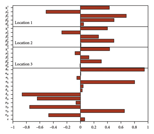
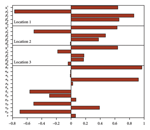
| Parameters | AD + CD | ITL + ITN + ITA | ||
|---|---|---|---|---|
| PRCC | p value | PRCC | p value | |
| ϵ | 0.0638 | 0.0468 | 0.0618 | 0.0539 |
| σD | −0.4702 | ≤0.0001 | −0.7006 | ≤0.0001 |
| υD | 0.6496 | ≤0.0001 | 0.3912 | ≤0.0001 |
| γD | −0.7530 | ≤0.0001 | −0.5108 | ≤0.0001 |
| μD | −0.0645 | 0.0444 | 0.0683 | 0.0331 |
| δD | −0.6403 | ≤0.0001 | −0.2912 | ≤0.0001 |
| δC | −0.8629 | ≤0.0001 | −0.5626 | ≤0.0001 |
| θA | 0.0283 | 0.3772 | 0.0023 | 0.9437 |
| μE | 0.0416 | 0.1947 | 0.0250 | 0.4360 |
| αE | 0.8030 | ≤0.0001 | 0.9235 | 0 |
| αL | −0.0527 | 0.1001 | −0.0071 | 0.8241 |
| αN | 0.0036 | 0.9112 | −0.0035 | 0.9125 |
| ϕT | 0.9466 | 0 | 0.9695 | 0 |
| −0.0070 | 0.8269 | −0.0396 | 0.2172 | |
| 0.3107 | ≤0.0001 | 0.1731 | ≤0.0001 | |
| 0.1252 | 0.0001 | 0.1774 | ≤0.0001 | |
| −0.0801 | 0.0125 | −0.1810 | ≤0.0001 | |
| K3 | 0.4308 | ≤0.0001 | 0.6394 | ≤0.0001 |
| 0.0066 | 0.8367 | −0.0083 | 0.7971 | |
| 0.4950 | ≤0.0001 | 0.3786 | ≤0.0001 | |
| 0.2678 | ≤0.0001 | 0.4716 | ≤0.0001 | |
| −0.2749 | ≤0.0001 | −0.5064 | ≤0.0001 | |
| K2 | 0.4011 | ≤0.0001 | 0.6311 | ≤0.0001 |
| 0.0476 | 0.1378 | 0.0014 | 0.9646 | |
| 0.4981 | ≤0.0001 | 0.6585 | ≤0.0001 | |
| 0.6794 | ≤0.0001 | 0.8616 | ≤0.0001 | |
| −0.5074 | ≤0.0001 | −0.7708 | ≤0.0001 | |
| K1 | 0.4292 | ≤0.0001 | 0.6408 | ≤0.0001 |
- With the movement scenario, the locations are connected.
Therefore, control strategies which target those parameters with significant PRCC values will give the greatest impact on the model response functions. For instance, a control that aims for a 10% decrease in the transmission probability in dogs in locations 1, 2, and 3 will lead to 49.8%, 49.5%, 31.1% reduction in infected dogs and about 65.8%, 37.9%, 17.3% reduction in infected ticks . Similarly a 10% decrease in the ticks transmission probability (βT) in locations 1, 2, and 3 will lead to 67.9%, 26.8%, 12.5% reduced infection in dogs and about 86.2%, 47.2%, 17.7% reduced infection in ticks. Also, a 10% deduction in tick biting rate (ϕT) will lead to about 94.7% reduction in infected dogs, and about 97% reduction in infected ticks. Lastly, a 10% increase in ticks death rate (μT) in locations 1, 2, and 3 will result in about 50.7%, 27.5%, 8% reduction in infected dogs and about 77.1%, 50.6%, 18.1% decrease in ticks.
4. Simulating the Ehrlichia chaffeensis Model (27)
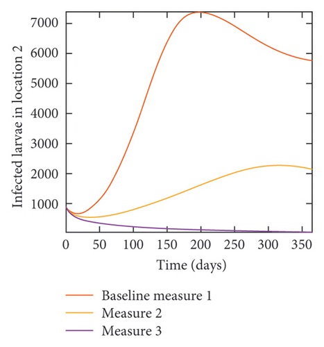
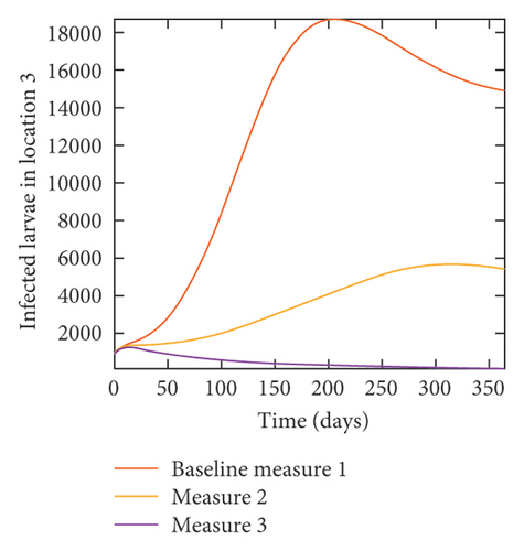
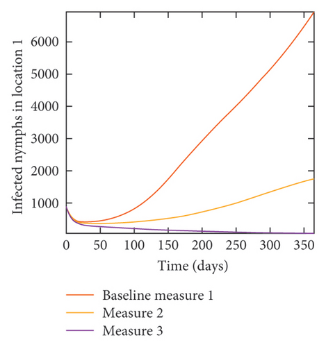
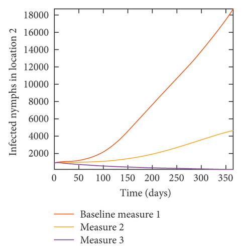
In this section, we would simulate the Ehrlichia chaffeensis model (27) when there are no movements between the three locations and when dogs and ticks move between the locations. Later on, we would use the results from the sensitivity analysis and simulate the Ehrlichia chaffeensis model (27) varying the transmission probabilities , and the ticks death rate . Then, we would analyze the effect of these parameters on the spread of Ehrlichia chaffeensis separately and jointly.
We start by simulating model (27) with no movement using parameters given in Table 2. We assume that infection is higher in location 1, followed by location 2, and location 3 has the least infection. As expected Figures 5(a) and 5(b) show higher number of acutely and chronically infected dogs in location 1, followed by locations 2 and 3; higher infected larvae, nymphs, and adult ticks were also observed in Figures 5(c), 5(d), and 5(e) in location 1, followed by locations 2 and 3.
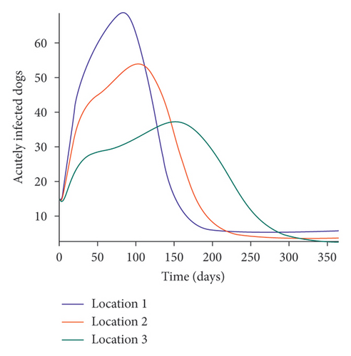
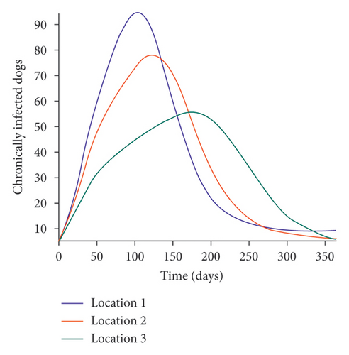
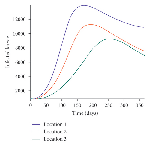
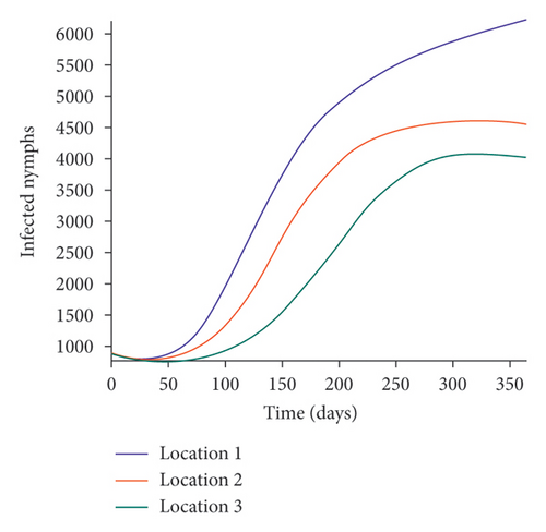
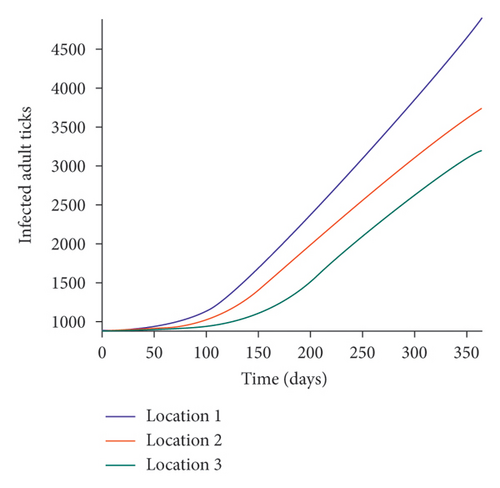
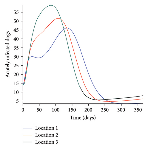
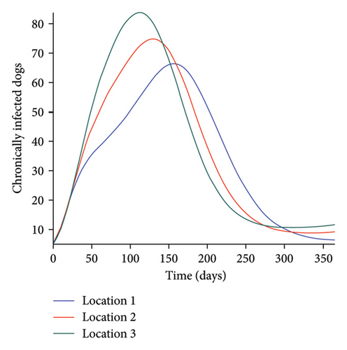
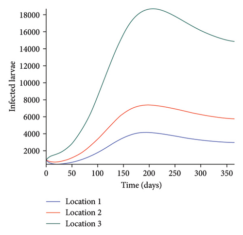
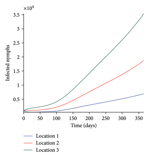
Next, we simulate model (27) with more movement into location 3 and least movement into locations 1 while infection remain higher in location 1 and smallest in location 3. With this scenario, Figures 6(a) and 6(b) show higher number of acutely and chronically infected dogs in location 3, followed by locations 2 then 1 even though infection is higher in location 1. Also, higher infected larvae, nymphs, and adult ticks were observed in location 3, followed by locations 2 and 1, see Figures 6(c), 6(d), and 6(e).
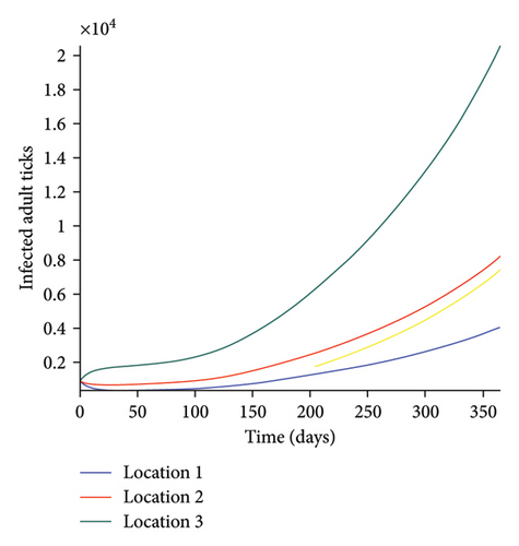
These results show the impact of movement on the transmission of the disease as dogs and ticks move across regions.
In the next section, we would use the results from the sensitivity analysis and simulate the Ehrlichia chaffeensis model (27) varying the transmission probabilities and the ticks’ death rate . We analyze jointly the effect of these parameters on the spread of Ehrlichia chaffeensis within the dogs and ticks populations. Note that it makes sense to explore the joint effect of these parameters since the outcome of the sensitivity analysis is only on the effect of one parameter at a time.
4.1. Effect of Disease Transmission and Ticks Natural Death
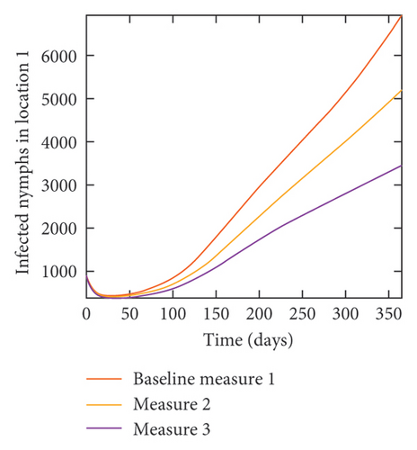
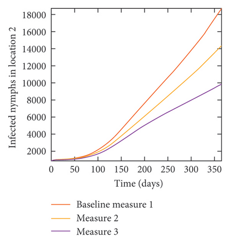
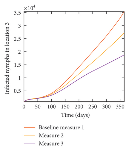
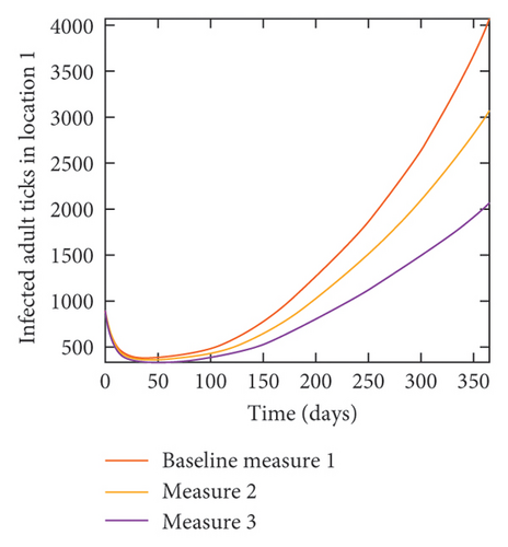
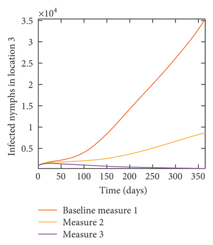
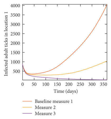
Here, we investigate the impact of disease transmission probabilities and the ticks death rate as control measures on infected dogs and ticks. We vary the values of the transmission probabilities and the number of ticks death rate and then examine the effect of these measures separately and jointly on the trajectories of infected dogs and ticks under several scenarios (i) when the three locations are isolated with no movement between them and control measures are implemented in each location and (ii) when the locations are connected with movement between and control measures are first implemented a location at a time and then implemented at once in all the locations.
4.2. Isolated Locations: Disease Transmission and Ticks Control
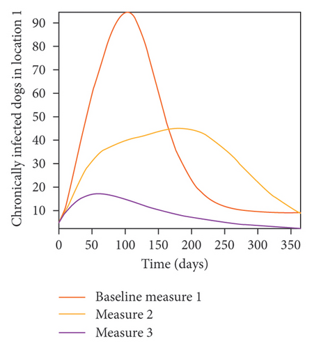
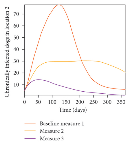
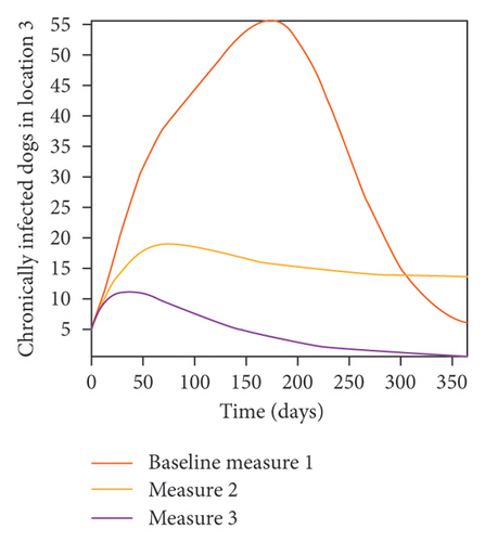
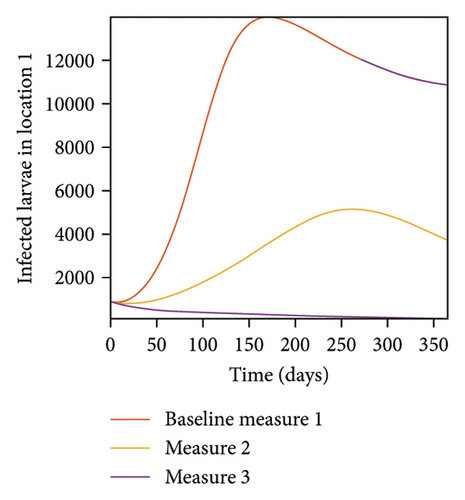
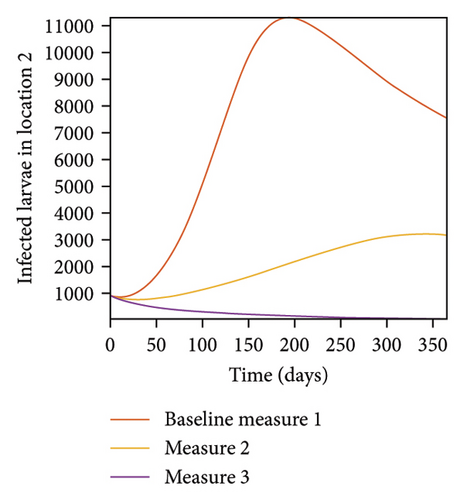
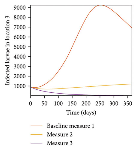
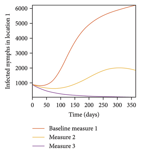
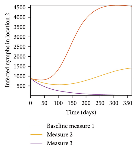
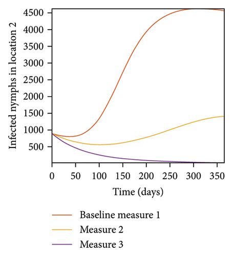
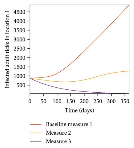
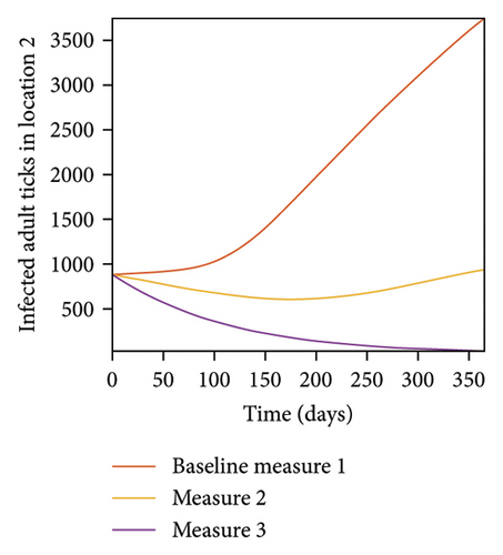
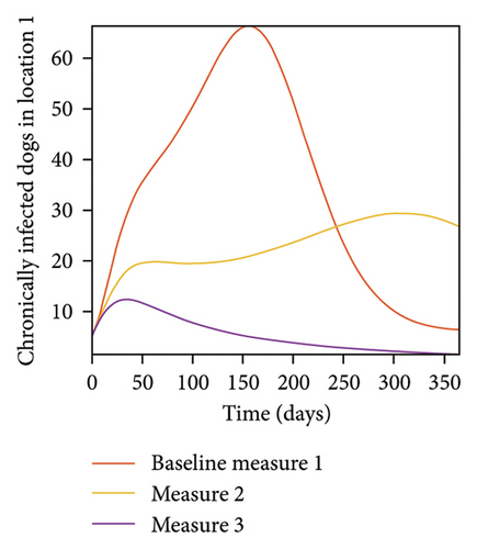
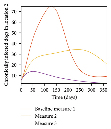
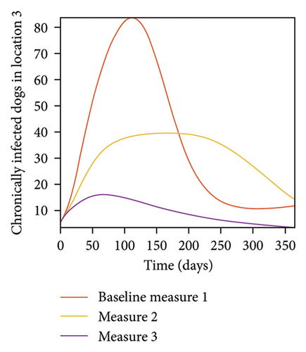
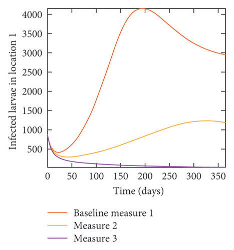
Here, we explore the combined effect of varying the transmission probabilities (, and ) and ticks natural death rate when there are no movements between the locations. However, infection is higher in location 1, followed by location 2, location 3 has the least infection. We considered three measures: (i) Measure 1 where the baseline parameters are used for , and , i = 1, 2, 3, as given in Table 2; (ii) Measure 2, the baseline parameter values for , are halved while the value for is doubled; and (iii) Measure 3, the baseline parameter values for are divided by four while the values for are multiplied by four.
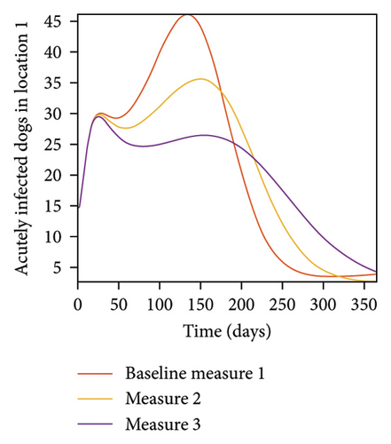
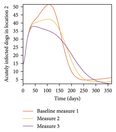
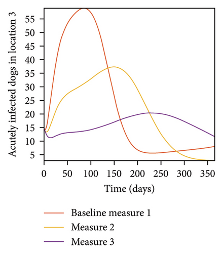
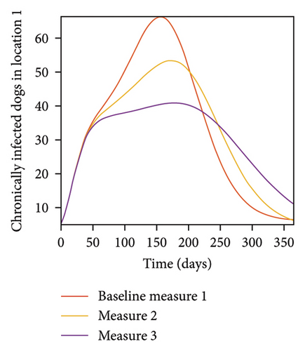
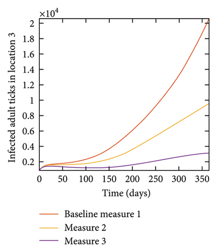
In Figure 7, we observed reduction in acutely and chronically infected dogs in each location as the control measures varies as described above; Figure 8 show the infected larvae, nymphs, and adult ticks in each locations. Table 6 show similar trends with the sum of the acutely and chronically infected dogs and ticks over the simulation period of 52 weeks representing a year.
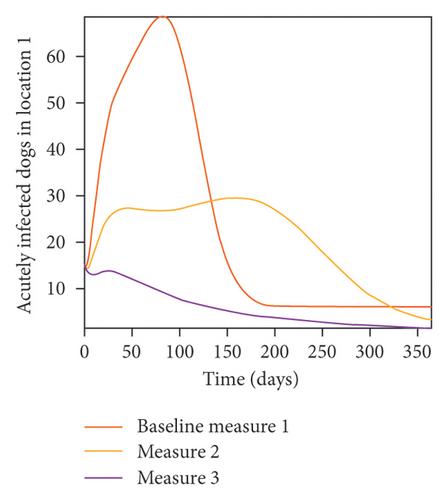
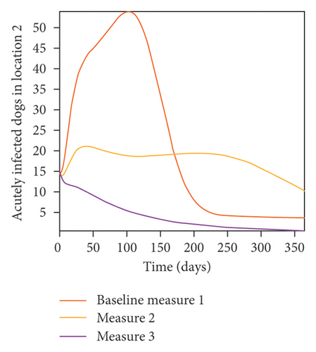
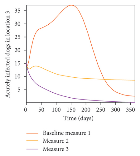

| Measures | Location 1 | Location 2 | Location 3 | |||
|---|---|---|---|---|---|---|
| 1 | 8.6860 × 10⁵ | 8.1537 × 10⁵ | 7.6898 × 10⁵ | |||
| 2 | 7.4407 × 10⁵ | 6.5097 × 10⁵ | 3.7349 × 10⁵ | |||
| 3 | 1.9840 × 10⁵ | 1.4660 × 10⁵ | 9.6643 × 10⁴ | |||
| 1 | 1.3523 × 10⁶ | 1.2787 × 10⁶ | 1.2063 × 10⁶ | |||
| 2 | 1.1570 × 10⁶ | 9.7318 × 10⁵ | 5.5894 × 10⁵ | |||
| 3 | 3.2066 × 10⁵ | 2.4321 × 10⁵ | 1.6682 × 10⁵ | |||
| 1 | 3.5822 × 10⁸ | 2.6880 × 10⁸ | 2.0342 × 10⁸ | |||
| 2 | 1.1852 × 10⁸ | 7.2714 × 10⁷ | 3.3064 × 10⁷ | |||
| 3 | 1.1374 × 10⁷ | 8.7850 × 10⁶ | 7.2365 × 10⁶ | |||
| 1 | 1.4126 × 10⁸ | 1.0978 × 10⁸ | 8.6427 × 10⁷ | |||
| 2 | 4.7045 × 10⁷ | 3.1790 × 10⁷ | 1.8848 × 10⁷ | |||
| 3 | 8.0034 × 10⁶ | 7.3395 × 10⁶ | 6.9439 × 10⁶ | |||
| 1 | 8.5854 × 10⁷ | 7.1381 × 10⁷ | 6.0548 × 10⁷ | |||
| 2 | 3.2641 × 10⁷ | 2.6498 × 10⁷ | 2.1308 × 10⁷ | |||
| 3 | 9.6459 × 10⁶ | 9.4308 × 10⁶ | 9.3019 × 10⁶ | |||
- Measure 1: used the baseline parameters for and , i = 1, 2, 3, as given in Table 2. Measure 2: the parameters for , are divided by two and are doubled. Measure 3: , values are divided by four and are multiplied by four.
This results show the importance of ensuring the infection rates are low in order to reduce the overall burden of the disease in each location.
4.3. Connected Locations: Control in One Location at a Time
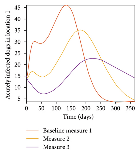
In this section, we explore the effect of varying the transmission probabilities (, and ) and ticks natural death rate when dogs and ticks can move freely between the locations. We assume the infection is higher in location 1, followed by locations 2, and 3; location 3 has the least infection. Here, we consider the scenario where the control measures are implemented a location at a time. We also considered three control measures 1,2, 3: with Measure 1, the baseline parameter values are used for , and , i = 1, 2, 3, as given in Table 2; with Measure 2, the baseline parameter values for , are halved while and is doubled; with Measure 3, the baseline parameter values for are divided by four while are multiplied by four.
4.4. Connected Locations: Control in Location 1 Only
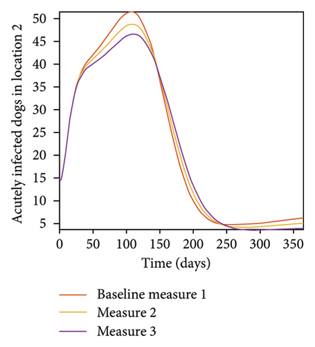
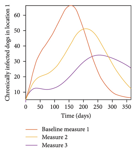
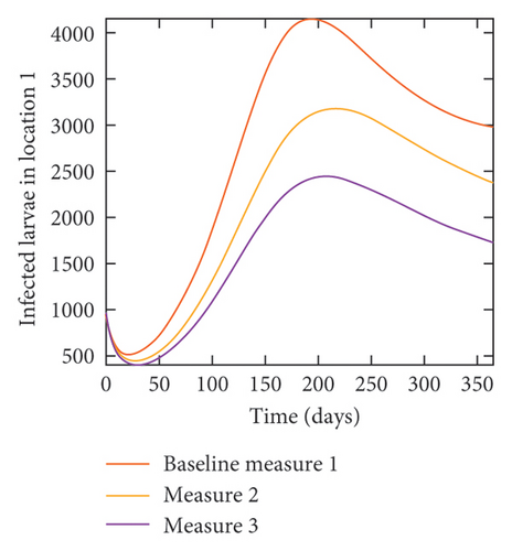
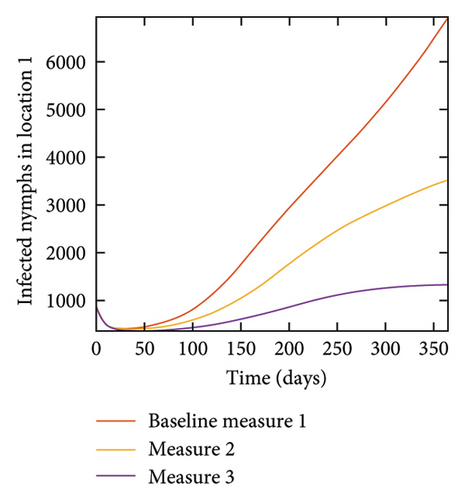
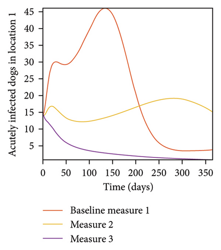
With this scenario the control measures described above are only implemented location 1. We observed in location 1, substantial reduction in population of acutely and chronically infected dogs as the control measures varies from Measures 1 through 3, see Figure 9. The effect of this measure trickles to locations 2 and 3 but the impact is minimal compare to the effect in location 1. Figure 10 shows the outcome for infected larvae, nymphs, and adult ticks in each location. Table 7 shows similar trends in the sum of the acutely and chronically infected dogs and ticks over the simulation period.
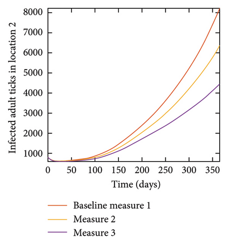

| Measures | Location 1 | Location 2 | Location 3 | |||
|---|---|---|---|---|---|---|
| 1 | 7.8998 × 10⁵ | 8.2910 × 10⁵ | 8.6320 × 10⁵ | |||
| 2 | 7.3806 × 10⁵ | 8.1344 × 10⁵ | 8.4190 × 10⁵ | |||
| 3 | 5.7417 × 10⁵ | 7.9930 × 10⁵ | 8.2301 × 10⁵ | |||
| 1 | 1.2379 × 10⁶ | 1.2905 × 10⁶ | 1.3359 × 10⁶ | |||
| 2 | 1.1365 × 10⁶ | 1.2705 × 10⁶ | 1.3089 × 10⁶ | |||
| 3 | 8.3462 × 10⁵ | 1.2531 × 10⁶ | 1.2859 × 10⁶ | |||
| 1 | 9.8522 × 10⁷ | 1.8229 × 10⁸ | 4.6149 × 10⁸ | |||
| 2 | 7.5886 × 10⁷ | 1.5423 × 10⁷ | 3.8438 × 10⁸ | |||
| 3 | 5.7685 × 10⁷ | 1.3168 × 10⁶ | 3.2258 × 10⁸ | |||
| 1 | 1.0240 × 10⁸ | 2.7218 × 10⁸ | 5.1081 × 10⁸ | |||
| 2 | 7.9835 × 10⁷ | 2.1841 × 10⁸ | 4.1087 × 10⁸ | |||
| 3 | 5.8344 × 10⁷ | 1.6843 × 10⁸ | 3.1871 × 10⁸ | |||
| 1 | 5.2300 × 10⁷ | 1.0372 × 10⁸ | 2.5791 × 10⁸ | |||
| 2 | 4.2156 × 10⁷ | 8.6180 × 10⁷ | 2.1335 × 10⁸ | |||
| 3 | 3.1419 × 10⁷ | 6.8570 × 10⁷ | 1.6840 × 10⁸ | |||
- Control measures are only implemented in location 1.
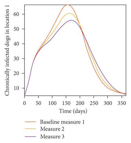
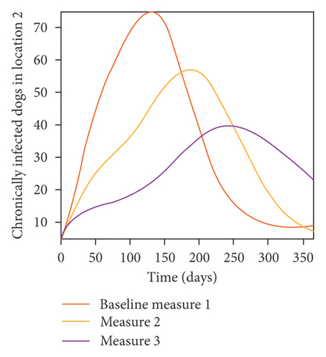
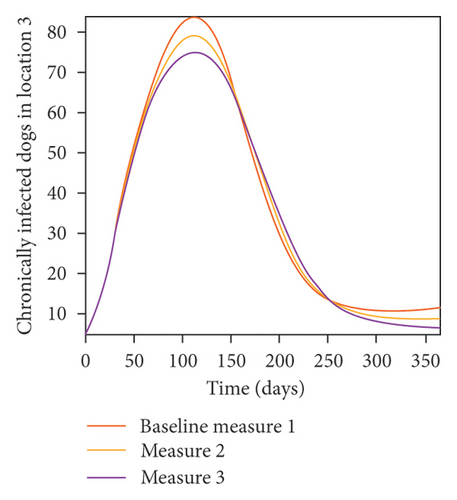
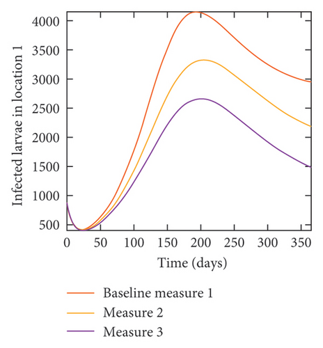
4.5. Connected Locations: Control in Location 2 Only
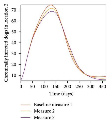
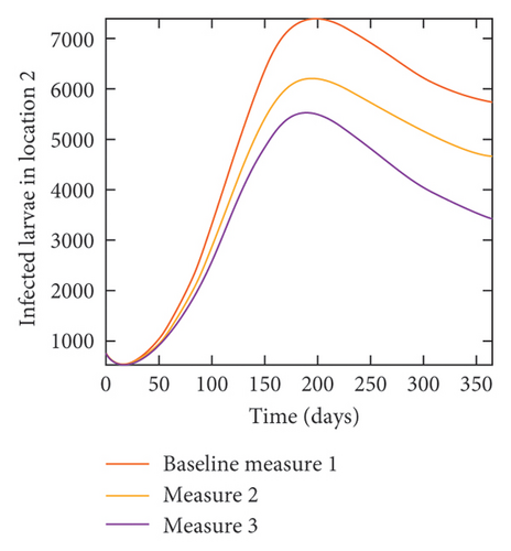
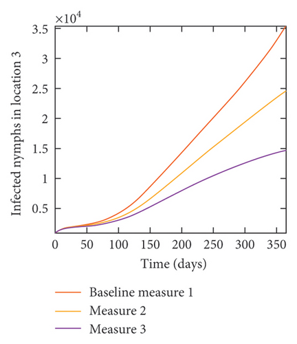
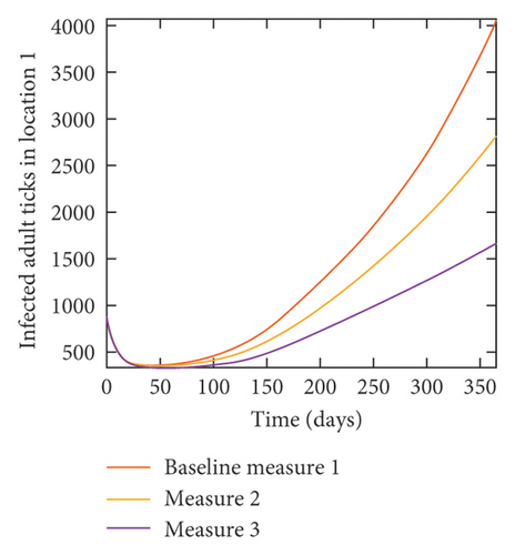
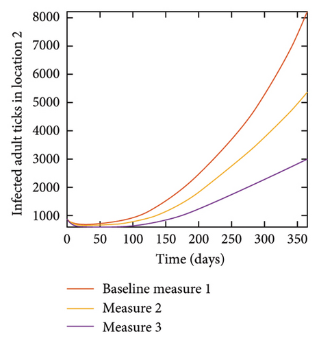
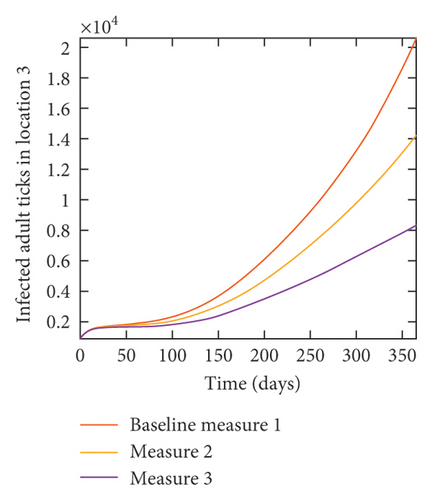
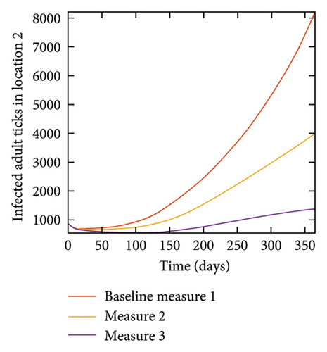
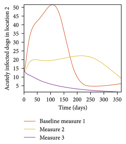
With this scenario the control measures described above are only implemented in location 2. Significant reduction in population of acutely and chronically infected dogs is observed in location 2 as the control measures varies from Measures 1 through 3, see Figure 11. The effect of this measure trickles to locations 1 and 3 but the impact is minimal compare to the effect in location 2. Figure 12 shows the outcome for infected larvae, nymphs, and adult ticks in each location. Similar trends can be seen in Table 8 in the values of the sum of the acutely and chronically infected dogs and ticks over the simulation period.
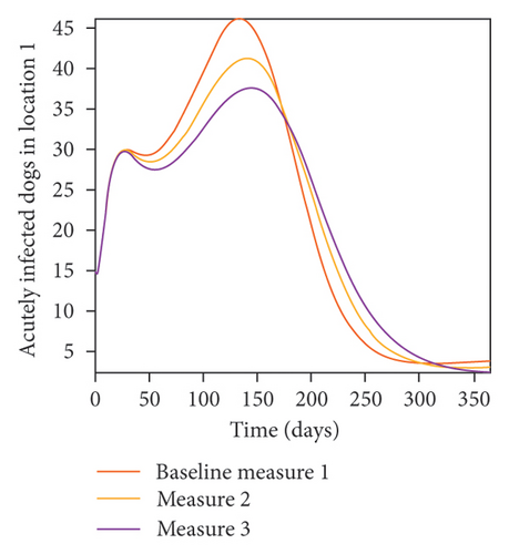
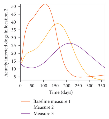
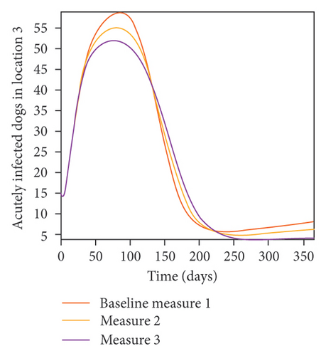
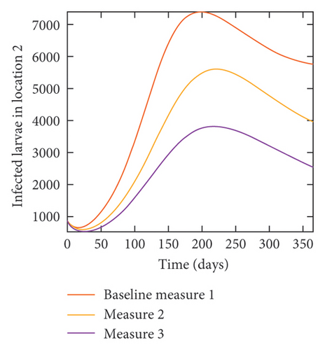
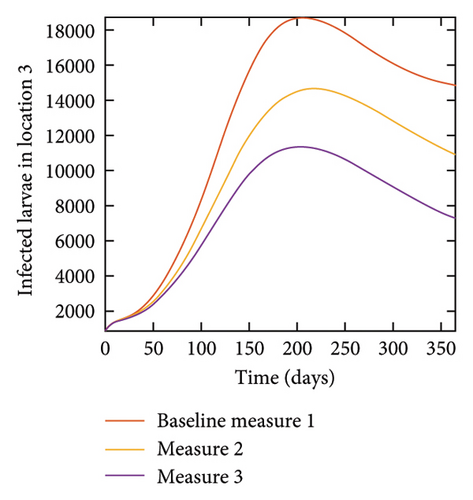
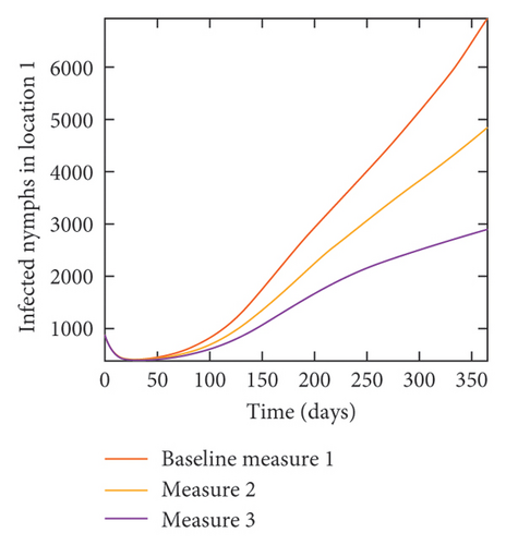
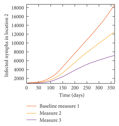
| Measures | Location 1 | Location 2 | Location 3 | |||
|---|---|---|---|---|---|---|
| 1 | 7.8998 × 10⁵ | 8.2910 × 10⁵ | 8.6320 × 10⁵ | |||
| 2 | 7.7723 × 10⁵ | 7.6326 × 10⁵ | 8.3576 × 10⁵ | |||
| 3 | 7.6435 × 10⁵ | 6.5388 × 10⁵ | 8.1033 × 10⁵ | |||
| 1 | 1.2379 × 10⁶ | 1.2905 × 10⁶ | 1.3359 × 10⁶ | |||
| 2 | 1.2197 × 10⁶ | 1.1930 × 10⁶ | 1.3011 × 10⁶ | |||
| 3 | 1.1996 × 10⁶ | 9.6952 × 10⁵ | 1.2695 × 10⁶ | |||
| 1 | 9.8522 × 10⁷ | 1.8229 × 10⁸ | 4.6149 × 10⁸ | |||
| 2 | 7.9056 × 10⁷ | 1.3233 × 10⁸ | 3.6249 × 10⁸ | |||
| 3 | 6.2368 × 10⁷ | 9.1858 × 10⁷ | 2.7911 × 10⁸ | |||
| 1 | 1.0240 × 10⁸ | 2.7218 × 10⁸ | 5.1081 × 10⁸ | |||
| 2 | 7.7780 × 10⁷ | 1.9816 × 10⁸ | 3.8444 × 10⁸ | |||
| 3 | 5.4568 × 10⁷ | 1.2939 × 10⁸ | 2.6622 × 10⁸ | |||
| 1 | 5.2300 × 10⁷ | 1.0372 × 10⁸ | 2.5791 × 10⁸ | |||
| 2 | 4.0332 × 10⁷ | 7.6112 × 10⁷ | 1.9685 × 10⁸ | |||
| 3 | 2.8382 × 10⁷ | 4.9422 × 10⁷ | 1.3647 × 10⁸ | |||
- Control measures are only implemented in location 2.
4.6. Connected Locations: Control in Location 3 Only
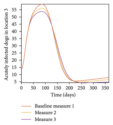
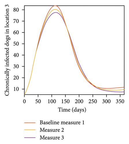
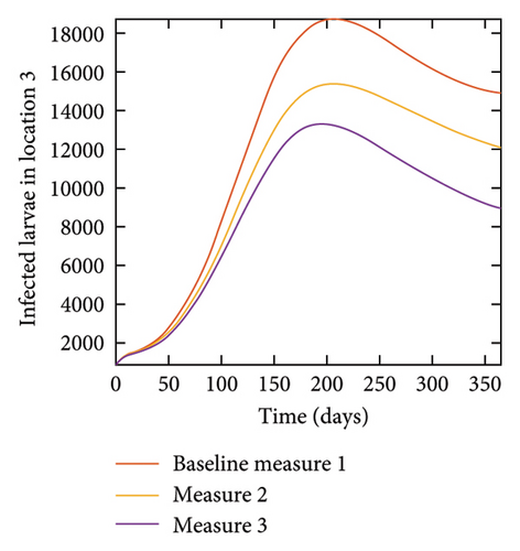
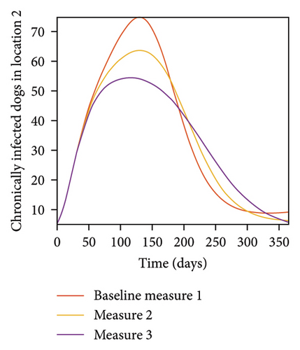
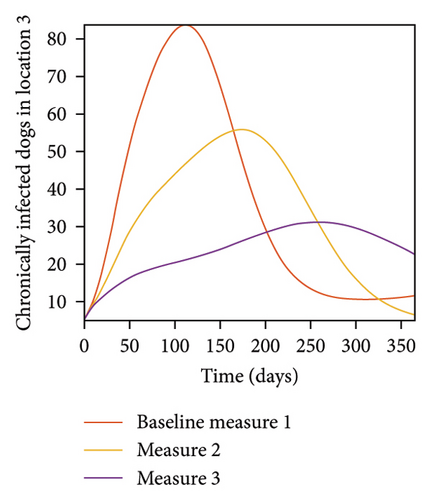
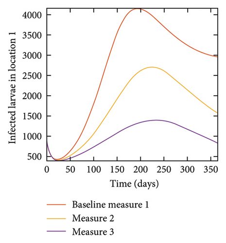
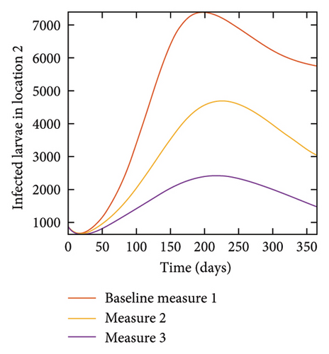
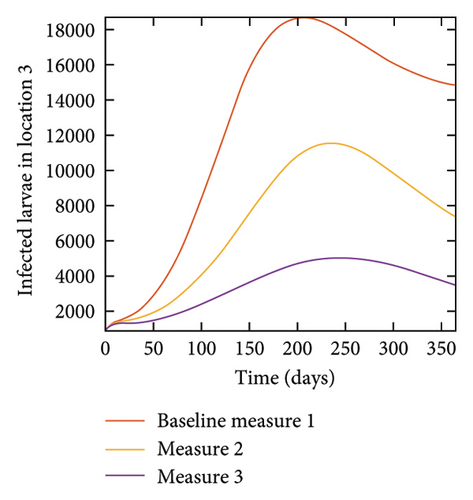
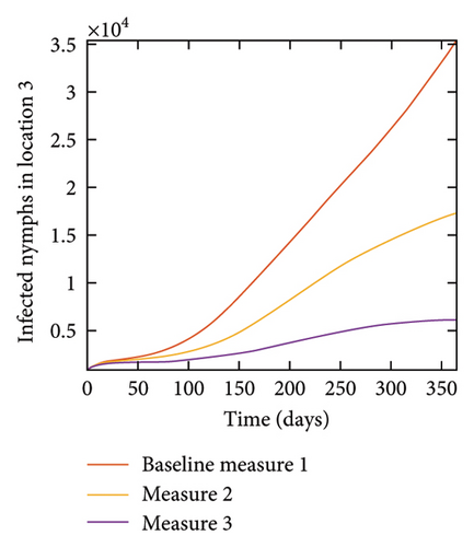
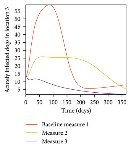
With this scenario the control measures are implemented in location 3 only. We observed in location 3, significant reduction in population of acutely and chronically infected dogs with changes in the control measures 1 through 3, see Figure 13. The effect of this measure trickles to locations 1 and 2 but the effect is minimal compare to the effect in location 3. Table 9 shows similar trends in the sum of the acutely and chronically infected dogs and ticks over the simulation period of 52 weeks. The outcome for infected larvae, nymphs, and adult ticks in each location are shown in Figure 14.
| Measures | Location 1 | Location 2 | Location 3 | |||
|---|---|---|---|---|---|---|
| 1 | 7.8998 × 10⁵ | 8.2910 × 10⁵ | 8.6320 × 10⁵ | |||
| 2 | 7.6634 × 10⁵ | 7.9359 × 10⁵ | 7.6814 × 10⁵ | |||
| 3 | 7.2907 × 10⁵ | 7.6287 × 10⁵ | 5.8953 × 10⁵ | |||
| 1 | 1.2379 × 10⁶ | 1.2905 × 10⁶ | 1.3359 × 10⁶ | |||
| 2 | 1.2013 × 10⁶ | 1.2441 × 10⁶ | 1.2033 × 10⁶ | |||
| 3 | 1.1267 × 10⁶ | 1.1978 × 10⁶ | 8.6925 × 10⁵ | |||
| 1 | 9.8522 × 10⁷ | 1.8229 × 10⁸ | 4.6149 × 10⁸ | |||
| 2 | 6.2381 × 10⁷ | 1.1297 × 10⁸ | 2.6367 × 10⁸ | |||
| 3 | 3.5622 × 10⁷ | 6.3083 × 10⁷ | 1.2774 × 10⁸ | |||
| 1 | 1.0240 × 10⁸ | 2.7218 × 10⁸ | 5.1081 × 10⁸ | |||
| 2 | 6.1195 × 10⁷ | 1.6251 × 10⁸ | 2.9118 × 10⁸ | |||
| 3 | 2.9903 × 10⁷ | 7.9561 × 10⁷ | 1.3070 × 10⁸ | |||
| 1 | 5.2300 × 10⁷ | 1.0372 × 10⁸ | 2.5791 × 10⁸ | |||
| 2 | 3.1708 × 10⁷ | 6.2339 × 10⁷ | 1.4865 × 10⁸ | |||
| 3 | 1.5584 × 10⁷ | 3.0333 × 10⁷ | 6.6731 × 10⁷ | |||
- Control measures are only implemented in location 3.


4.7. Connected Locations: Control at all Locations at the Same Time
With this scenario the three control measures described above are implemented in all three locations at the same time. We observed in all three locations significant reduction in population of acutely and chronically infected dogs using the three control measures, Measure 3 produced the most reduction see Figure 15. It is interesting to note that since similar levels of control are implemented in all three locations the effect of movement is cancelled out, as the sum of infected under this scenario is the same as the case with no movement. Similar trends are seen in Table 10 in the sum of acutely and chronically infected dogs and ticks over the simulation period. The outcome for infected larvae, nymphs, and adult ticks in each location are shown in Figure 16.
| Measures | Location 1 | Location 2 | Location 3 | |||
|---|---|---|---|---|---|---|
| 1 | 8.6860 × 10⁵ | 8.1537 × 10⁵ | 7.6898 × 10⁵ | |||
| 2 | 7.4407 × 10⁵ | 6.5097 × 10⁵ | 3.7349 × 10⁵ | |||
| 3 | 1.9840 × 10⁵ | 1.4660 × 10⁵ | 9.6643 × 10⁴ | |||
| 1 | 1.3523 × 10⁶ | 1.2787 × 10⁶ | 1.2063 × 10⁶ | |||
| 2 | 1.1570 × 10⁶ | 9.7318 × 10⁵ | 5.5894 × 10⁵ | |||
| 3 | 3.2066 × 10⁵ | 2.4321 × 10⁵ | 1.6682 × 10⁵ | |||
| 1 | 3.5822 × 10⁸ | 2.6880 × 10⁸ | 2.0342 × 10⁸ | |||
| 2 | 1.1852 × 10⁸ | 7.2714 × 10⁷ | 3.3064 × 10⁷ | |||
| 3 | 1.1374 × 10⁷ | 8.7850 × 10⁶ | 7.2365 × 10⁶ | |||
| 1 | 1.4126 × 10⁸ | 1.0978 × 10⁸ | 8.6427 × 10⁷ | |||
| 2 | 4.7045 × 10⁷ | 3.1790 × 10⁷ | 1.8848 × 10⁷ | |||
| 3 | 8.0034 × 10⁶ | 7.3395 × 10⁶ | 6.9439 × 10⁶ | |||
| 1 | 8.5854 × 10⁷ | 7.1381 × 10⁷ | 6.0548 × 10⁷ | |||
| 2 | 3.2641 × 10⁷ | 2.6498 × 10⁷ | 2.1308 × 10⁷ | |||
| 3 | 9.6459 × 10⁶ | 9.4308 × 10⁶ | 9.3019 × 10⁶ | |||
- Control measures are implemented in all three locations 1, 2, and 3.


5. Discussion, Conclusion, and Recommendations
5.1. Discussion
In this paper we developed and analyzed a mathematical model (14) for the disease transmission dynamics of Ehrlichia chaffeensis in dogs using the natural history of infection of the disease. Features of this model include the different life stages of ticks and the different infectious stages of both dogs and ticks. The life stages of the ticks included eggs, larvae, nymphs, and adults which typically take over a two year span to complete. The infectious stages of the dogs were divided into acute and clinical/chronic. The first 2–4 weeks of infection is referred to as the acute stage. After the initial 2–4 weeks if not treated the dog will progress into a clinical/chronic stage, this stage typically leads to death [2]. Ehrlichia chaffeensis is a serious tick-borne infectious disease that can cause life-threatening complications. It is important to know how to prevent dogs from being infected with Ehrlichia chaffeensis and to be aware of the symptoms if dog becomes infected. One primary vector of Ehrlichia chaffeensis is the Amblyomma americanum ticks.
We extend the Ehrlichia chaffeensis model (14) by incorporating visitation and long distance migratory movements for dogs and ticks. Owners typically take their dogs on hikes or to dog parks. It is estimated that people take their dogs on a walk about 9 times a week for around 34 minutes. This usually ends up being a two mile walk. This totals to about 370 miles a year [40]. The short dog movements were captured through the visitation parameters pij, which is the proportion of time a dog in location i spends visiting location j. Ticks long distance migratory movement may be due to ticks dropping off after feeding on either migratory birds moving north or from white-tail deer or other larger mammals [31].
Quantitative analysis of models (14) and (27) indicate that the disease-free equilibrium of these models is locally asymptotically stable when their reproduction number is less than one. Following [39], we can show that the global reproduction number of model (27) is bounded below and above by the local reproduction numbers from the patch with least and most transmission dynamics.
Next, we carried out a global sensitivity analysis using LHS/PRCC method to determine the parameter with the most influence on the response functions of sum of acutely and chronically infected (AD + CD) and the sum of infected ticks in all life stages (ITL + ITN + ITA). To implement the analysis, we used both models (14) and (27), and parameter values obtained from literature in most cases as well as assumed some where we could not find their values. The significant parameters for model (27) with movement between the locations are disease progression rate in dogs (σD), the rate (υD) dogs progress to chronic infection from acute infection, dog recovery rate (γD), the natural death rate of dogs (μD), death rate (δD) of acutely infected dogs, death rate of the chronically infected dogs (δC), birth rate of dogs , the maturation rates eggs to larvae (αE), the tick biting rate , the dog transmission probability (βD), the tick transmission probability and death rate of ticks , and the carrying capacity Ki. There parameters are also significant when we used model (14) that models transmission dynamics in a single location, see Figure 2.
Furthermore, we observed in Figures 3 that the PRCC values of parameters , Ki, , , and are relatively the same when there are no movement between the region. However, with movement the PRCC values for parameters , Ki, , , and are different, with those in location 1 having higher values than those in locations 2 and 3 since there is more movement into location 1, than 2 and 3, see Figure 4. Knowing these significant parameters is essential to the formulation of effective control strategies for combating the spread of disease. For instance, a control that aims for a 10% decrease in the transmission probability in dogs (βD) will lead to 88% reduction in sum of acutely and chronically infected dogs and about 78% reduction in infected ticks of all life stages. Similarly a 10% decrease in the ticks’ transmission probability (βT) will lead to 71.4% reduced infection in dogs and about 83% reduced infection in ticks. Also, a 10% deduction in tick biting rate (ϕT) will lead to about 95% reduction in infected dogs, and about 94% reduction in infected ticks. Furthermore, a 10% increase in ticks death rate (μT) will result in about 72.4% reduction in infected dogs and about 83.4% decrease in ticks.
The simulation results of model (27) in Figure 5 show that locations with high infection rates like location 1 have a high number of infected dogs and ticks. This is due to the fact that the infected dogs and ticks are not moving the disease to other locations but keeping it localized in their home location. On the other hand, locations with high movement and visitation rates see an increase in infected dogs and ticks. This is due to infected dogs and ticks traveling and infecting the dogs and ticks within the location that they are visiting (in the case of dogs) and moving to (in the case of ticks). In Figures 6(a) and 6(b), we see higher number of acutely and chronically infected dogs in location 3, followed by location 2 then location 1 even though infection is higher in location 1. Similar result is observed for infected larvae, nymphs, and adult ticks in Figures 6(c), 6(d), and 6(e). These results show the impact of movement on the transmission of the disease as dogs and ticks move across locations. This result align with results in [38, 39], where the patch with the highest host movement or migration have the most infection. For instance Nguyen et al. [38] showed that deer mobility from a Lyme disease endemic county into Lyme disease free county will lead to the emergence of the disease in this second county free of the disease. Similarly, Zhang et al. [39] showed that rodent migration between patches can promote the disease spreading within all patches.
Next, we use the results from the sensitivity analysis coupled with movement between the locations to determine which control measure reduces the spread of Ehrlichia chaffeensis the most among dogs and ticks. Identifying these measures is crucial to decreasing the spread of Ehrlichia chaffeensis amongst dogs. We note that during the single location control, the effect trickles to other locations due to the effect of movement between the locations. To see the impact of this single location control trickling effect, we compare in location 2 the effect of the control measures in location 1 only where the transmission is highest to the control measures in location 3 only where movement into it is highest, but transmission is lowest, we observed that controlling in location 3 only produces the most reduction in location 2. For instance, Measure 3 for acutely infected dogs in location 2 with location 1 only control is , while acutely infected dogs in location 2 with location 3 only control is . Similarly for the chronically infected dogs, we have in location 2 with location 1 only control, while with location 3 only control. See Tables 5 and 7 for the other dogs and ticks variables.
5.2. Conclusion
- (i)
The sensitivity analysis indicates that the response functions of sum of acutely and chronically infected (AD + CD) and the sum of infected ticks at all life stages (ITL + ITN + ITA) with and without movement between the locations are impacted by disease progression rate in dogs, progression rate to chronic infection in dogs, dog recovery rate, the natural death rate of dogs, disease induced death rate acutely and chronically infected dogs, birth rate of dogs, eggs maturation rates, tick biting rate, transmission probabilities in dogs and ticks, death rate of ticks, and the location carrying capacity.
- (ii)
In the absence of movement, locations with high infection rates have a high number of infected dogs and ticks; while locations with high movement rates see an increase in infected dogs and ticks
- (iii)
In the single location control, the effect of the control measures which reduces infection trickles to other locations due to the effect of movement between the locations. Furthermore, most infection reduction trickling effect is observed in location with the most movement.
5.3. Recommendations
- (a)
Dog movement: Dog owners should limit unnecessary travel with their dogs between locations, particularly if one area has a high prevalence of Ehrlichia chaffeensis infection, as restricting movement can lower the risk of exposure to infected ticks. They should also be mindful of areas with high infection rates and strive to avoid them when possible. Instead, opting for safer locations with lower tick populations, such as parks, for outdoor activities with their dogs. Additionally, practicing responsible pet management by keeping dogs on a leash during walks can prevent them from wandering into tick-abundant areas with dense vegetation.
- (b)
Tick prevention measures: Dog owners should use tick prevention products recommended by veterinarians, such as topical treatments, collars, or oral medications, to protect their dogs from tick bites. They should regularly check their dogs for ticks after outdoor activities and promptly remove any ticks found. If dog owners must travel with their dogs to areas with different infection rates, they should closely monitor their health for any signs of illness, such as lethargy, fever, loss of appetite, or lameness. And promptly seek veterinary attention if they suspect tick-borne disease.
- (c)
Regular veterinary check-ups: Dog owners should schedule routine veterinary check-ups for their dogs to monitor their health status and screen for tick-borne diseases. Early detection and treatment of infections can improve outcomes and prevent the spread of disease.
These recommendations aim to help dog owners mitigate the risk of Ehrlichia chaffeensis and other tick-borne diseases on their pets by implementing proactive measures and promoting responsible pet care practices [41].
Conflicts of Interest
The authors declare that there are no conflicts of interest regarding the publication of this paper.
Acknowledgments
This project was supported by the National Science Foundation under the EPSCOR Track 2 Grant no. 1920946.
Appendix
A. Proof of Lemma 1
Proof. Let t1 = sup{t > 0 : F(t) > 0 ∈ [0, t]}. Thus, t1 > 0. It follows from the first equation of the system (14), that
Hence,
Similarly, it can be shown that F > 0 for all t > 0.
For the second part of the proof, note that 0 < SD(0) ≤ ND(t), 0 ≤ ED(0) ≤ ND(t), 0 ≤ AD(0) ≤ ND(t), 0 < CD(0) ≤ ND(t), 0 ≤ RD(0) ≤ ND(t), 0 < STE(0) ≤ K, 0 < STL(0) ≤ NT(t), 0 ≤ ITL(0) ≤ NT(t), 0 < STN(0) ≤ NT(t), 0 ≤ ITN(0) ≤ NT(t), 0 < STA(0) ≤ NT(t), 0 ≤ ITA(0) ≤ NT(t).
Adding the dog and tick component of the Ehrlichia chaffeensis model (14) gives
We suppose that SE < K, where K is the carrying capacity.
Hence,
B. Proof of Lemma 2
Lemma 2. The region is positively-invariant for the model (14) with non-negative initial conditions in .
Proof. It follows from the sum of the first five equations of model (14) that
Hence, dND(t)/dt ≤ 0, if ND(0) ≥ θD/μD. Thus,
In particular, if ND(0) ≤ θD/μD, then ND(t) ≤ θD/μD.
Next, the last seven equations of model (14) give the following after summing the equations representing the larvae, nymphs, and adult stages
Thus,
Furthermore, if NT(0) ≤ σEK/μT, then NT(t) ≤ σEK/μT.
Equations (B.2) and (B.5) imply that ND(t) and NT(t) are bounded and all solutions starting in the region Ω remain in Ω. Thus, the region is positively-invariant and hence, the region Ω attracts all solutions in .
C. Basic Qualitative Properties of Model (27)
C.1. Positivity and Boundedness of Solutions
For the Ehrlichia chaffeensis transmission model (27) to be epidemiologically meaningful, it is important to prove that all its state variables are non-negative for all time. In other words, solutions of the model system (27) with non-negative initial data will remain non-negative for all time t > 0.
Lemma C.1. Let the initial data (0) ≥ 0, where . Then, the solutions F(t) of the Ehrlichia chaffeensis model (27) are non-negative for all t > 0. Furthermore,
Proof. Let t1 = sup{t > 0 : F(t) > 0 ∈ [0, t]}. Thus, t1 > 0. It follows from the seventh equation of system (27), that
Similarly, it can be shown that F > 0 for all t > 0.
For the second part of the proof, note that .
Considering the dog and tick components of model (14), we have
Now, summing separately the dog and tick components, gives
Thus, equation (C.8) leads to the following
C.2. Invariant Regions
The Ehrlichia chaffeensis model (27) will be analyzed in a biologically-feasible region as follows. Consider the feasible region
Lemma C.2. The region is positively-invariant for the Ehrlichia chaffeensis model (27) with non-negative initial conditions in .
Proof. The following steps are followed to establish the positive invariance of Ωi (i.e., solutions in Ωi remain in Ωi for all t > 0). The rate of change of the total dog and tick populations is obtained by adding separately the dog and tick component of model (27) for a particular region
From (C.15), and using a standard comparison theorem [42], we can show that
Furthermore, if , then and , if .
Thus, the region Ω is positively-invariant. Hence, it is sufficient to consider the dynamics of the flow generated by (27) in Ωi. In this region, the model is epidemiological and mathematically well-posed [14]. Thus, every solution of the basic model (27) with initial conditions in Ω remains in Ω for all t > 0. Therefore, the ω-limit sets of system (27) are contained in Ωi. This result is summarized below.
D. Stability of Disease-Free Equilibrium (DFE)
In the next section, the conditions for the existence and stability of the disease-free equilibrium of the model Ehrlichia chaffeensis (27) are stated.
The stability of can be established using the next generation matrix method on system (27). Taking ED, AD, CD, ITL, ITN, and ITA as the infected compartments and then using the aforementioned notation, the Jacobian and matrices for new infectious terms and the remaining transfer terms, respectively, are defined as.
The following result is established using Theorem 2 in [12].
Lemma D.1. The DFE of the Ehrlichia chaffeensis model (27) with movement, given by , is locally asymptotically stable (LAS) if , and unstable if .
The basic reproduction number measures the average number of new infections generated by a single infected individual (tick or dog) in a completely susceptible population [6, 16, 20, 39]. Thus, Lemma D.1 implies that malaria can be eliminated from the human population (when ) if the initial sizes of the subpopulations are in the basin of attraction of the DFE, .
Open Research
Data Availability
No dataset was used in this study.


