Adept Domestic Energy Load Profile Development Using Computational Intelligence-Based Modelling
Abstract
Most studies undertaken on energy usage in buildings have shown that energy utilization is widely influenced by occupancy presence and occupants’ activities relative to the indoor environment, which may be widely dependent on weather conditions and user behaviors. However, the core drawback that has negated the proficient estimation of energy is the modelling of occupant behavior relative to energy use. Occupants’ behavior is a complex phenomenon and has a dynamic nature influenced by numerous internal, individual, and circumstantial factors. This research proposes a computational intelligence-based model for household electricity usage profile development as impacted by core input variables—household activities, household financial status, and occupancy presence. The incorporation of these variables and their adaptiveness is expected to address and resolve unpredictability or nonlinearity concerns, thus allowing for adept energy usage estimation. The model addresses issues unresolved in many other studies, such as occupancy determination (deduction) and the impact on energy consumption. The performance precision of this approach has been demonstrated by trend series analysis, demand analysis, and correlation analysis. Based on the performance indicators including mean absolute percentage error (MAPE), mean square error (MSE), and root mean square error (RMSE), the model has shown proficient predictive output with respect to the metered (actual) energy usage data. The proposed model, compared to actual data, showed that average MAPE values for the respective day standard, morning peak, and night peak demand period (TOUs) are 2.8%, 1.88%, and 0.31% for all income groups, respectively. The aptitude to improve on energy prediction and evaluation accuracy, especially in these periods, makes it a highly suited tool for demand-side management, power generation, and distribution planning activity. This will translate into power system reliability, reduce operation cost (lowest cost), and reduce greenhouse emissions (environmental pollution), thereby cumulating into sustainable cities.
1. Introduction
It is well known that energy consumption prediction is a key element for utility power system planning. Furthermore, energy management systems can ensure an increase in the balance between supply and demand while contributing the issue of peak reduction especially unscheduled energy usage periods (time-of-use) as widely reported [1]. However, the accomplishment of such an objective presently in the residential sector is a challenging task due to the ever-fluctuating demand profile as a result of human activities and occupant behavior. Individual occupants’ behavior/activities are complex and have an impact on energy usage although they are not reflected in many practices resulting in poor energy prediction [2]. Occupancy of buildings by inhabitants is a vital aspect in building energy simulation; however, occupancy is difficult to represent owing to its temporal and spatial stochastic nature [3, 4].
Occupancy and occupants’ activities are replicated in most simulation models as simplistic, linear, and predetermined inputs. Furthermore, occupants’ activities have been reduced to fixed schedule usage of equipment/appliances and lighting usage based on existing historical data. The resultant deduction is at variance with the actual demand per dwelling in relation to the occupants’ activities. As a result of misalignment and high error arising from demand estimation along the time-of-use periods, interest in the energy load model development investigation has dwindled since it is almost impossible (due to associated metering cost, dwelling electrification, distribution board connection, etc.) to obtain individual appliance load profiles for the determination of the dwelling demand profile per dwelling. Published literature has also shown that occupancy is a critical factor that needs to be considered while determining domestic household demand. However, most simulation tools are grounded on fixed design profiles, making these inputs a concerted average of the whole dwelling that diverges from real occupancy. As a result, the obtained simulation outcomes are inaccurate due to the deficiency of the internal loads that represent household energy usage. Residential load profiles are essential in a range of planning, design, and management activities in power utilities.
The world has been facing challenges due to high energy demand [5], ever-increasing demand for energy, limitations of fossil fuel resources, and concerns about sustainability [6]. As a result, seasonal load shedding has been experienced in many developing countries, although strategies for demand-side management (DSM) are duly employed. The demand-side management (DSM) initiatives were widely implemented to attempt to modify the system load profile and for energy demand reduction while maintaining a tolerable level of electricity generation without offsetting occupants’ comfort and service delivery [7]. Such DSM interventions that were widely employed in domestic designs and operations include load shifting, strategic conservation, and peak clipping [7]. Yet, such methods are not fully effective as it is extremely hard to choose the optimum DSM technique for a distribution area without understanding occupants’ activities and occupancy and energy usage per occupant [8]. Major components or variables inherent in an energy system make it practically impossible to analyze without oversimplification. Therefore, it is crucial to consider factors that influence household energy consumption patterns to ascertain proficient energy estimation [9]. Such variables are essential in the assessment of demand management initiatives and load profile development.
Several prediction models have been presented for energy building consumption reduction, namely, white (engineering approaches), grey (statistical or hybrid approaches), and black-box models (data-driven machine learning or artificial intelligence- (AI-) based approaches) [8, 10]. However, these models are still deficient with respect to the proficient estimation of building consumption. Irrespective of the progress made in the residential building sector and building energy performance, the energy community still lacks a reliable and simple instrument that can instantaneously address and solve the energy and environmental balance of buildings. This may be due to current energy simulation tools being dependent on thermal factors such as climate and weather to predict energy consumption instead of looking into influential factors such as occupants’ activities and occupancy.
To bring about an improved solution to address such an issue, several works have pointed to the need for occupants’ behavior pattern classification based on income levels, household size, occupancy status, occupants’ activities, and possibly the associated vicinity [11]. The occupant behaviour is difficult to analyze without excessive simplicity due to its high complexity [12], as the current simulation tools have based the occupant behaviour on fixed patterns, while they do not take into account the activities of individual occupants, but instead adopt unspecific user schedules, which do not directly reflect the randomness of the occupant’s behaviour over time [8]. However, it is crucial to consider personalized occupants’ behavior/activities as they have an impact on energy loads to eliminate poor energy prediction. The incorporation of human behavior such as occupancy-interlinked inhabitant behavior and their impact on residential buildings is a necessity; presently there is no energy program for an all-inclusive and interlinked set of models that consider every aspect of occupants’ activities and presence.
The main objective of this research is to investigate an appropriate model that can address and solve problems related to demand forecast accuracy (i.e., reduce errors associated with demand profile estimation). The significance of occupants’ activities, occupancy presence, and income categories to enhance the energy load prediction accuracy will be demonstrated. The research work employs an artificial neural network to model residential energy usage profiles as influenced by key characteristic variables. Yan et al. in their study, they concluded that the Al-based approach tends to solve uncertainties associated with occupant behavior, highly reliable, and has the ability to deal with combined variables in building energy consumption predictions [4]. Another study indicated that smart optimization techniques based on Al are the future of optimization due to parallel processing, pattern recognition, and better decision-making capability [13]. The application of such variables reinforces the ANN model to handle uncertainty and volatility of data to ascertain proficient forecasting of energy load profiles. The study objective is expected to be achieved by developing a feed-forward backpropagation neural network (FFNN) model trained by the Levenberg–Marquardt learning algorithm with the incorporation of input variables, namely, income, occupants’ occupancy, and household actions. The proposed model has demonstrated various ways in which occupants occupy their dwellings and interact with household appliances and the importance of such interactions on proficient energy usage profile development. Furthermore, the proposed solution is expected to assist energy managers/planners in contributing to the United Nations Sustainable development goals with emphasis on energy poverty reduction (1), affordable energy (7), innovation (9), and sustainable cities (11).
- (i)
The development of an ANN-based residential energy load profile model hinged on income grouping and occupancy-interlinked occupant behavior variables.
- (ii)
The developed model was able to address and solve problems related to the accuracy of demand forecasting and reduced errors in residential energy load profiles. The improved accuracy emanated from various influential parameters such as occupants’ activities and occupancy presence being considered, and such parameters impact energy usage.
- (iii)
For optimal generation and cost-effectiveness relative to economic dispatch, demand in terms of the time of use periods (TOU) is of essence (core). Using average demand deduced from total energy consumption impacts the power systems network and laterally translates into error-prone demand forecast used in generation and distribution planning, thereby contributing to system strain, undergeneration or overgeneration, voltage issues, losses, etc. Furthermore, researchers have highlighted the need to bring about improved solutions around discrepancies arising between the actual and the predicted energy data as proffered in available resources. The developed model was able to minimize the discrepancy in energy usage prediction.
- (iv)
The proposed model was able to reduce assumptions around occupancy periods (fixed schedules of occupancy), i.e., repeated TOU models.
- (v)
The developed model with inclusive characteristic variables such as income, occupancy, and occupants’ activities was able to derive meaning and extract patterns from the complex nature associated with residential energy usage.
The study paper outline (structure) consists of the investigation approach—ANN structure, model process design strategy, investigation material and analysis, ANN prediction model, validation in terms of correlation analysis, trend analysis, and demand computation analysis. Lastly, the proposed model’s applicability and effectiveness are evaluated.
2. Method of Investigation
2.1. Investigation Method: Artificial Neural Network-Based Model
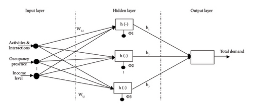
Due to volatility and nonlinearity associated with energy consumption, as well as its dependence on numerous driving factors, predicting energy consumption remained a challenging task [8], hence the need to bring into perspective methods that can address or be infused with. The black-box approach often referred to as data-driven machine learning or artificial intelligence- (AI-) based approach is one such method most widely applied in practice [8]. Black-box models are intelligence-based because of their ability to learn how to build energy-related output without prior knowledge of its internal relationship [14]. Al techniques empower devices, machines, etc. to simulate intellectual behavior, observe environment, reason, learn, and independently make decisions. These aptitudes make AI an ideal tool for addressing complexities associated with energy areas and usage, where massive amounts of data are to be analyzed, patterns identified, and decisions made [15]. Among intelligent- (AI-) based family, ANN models have gained popularity due to their compatibleness with nonlinear and ambiguous systems. A typical ANN has a structure that has same the structure of “neurons,” also called processing element, separated into three layers, namely, input, hidden, and output layer, as illustrated in Figure 1.
2.2. Model Process Design Strategy
The process design strategy for energy load profile model development is shown in Figure 2.

ANN as a random function approximation tool due to its ability to model compound relations among inputs and outputs is applied. ANN can be formulated by three processes, namely, the interconnection pattern between neurons of three layers; the learning process of weights; and the conversion of neuron’s weighted input to output by the activation function. The number of hidden layer neurons determines the accuracy of the prediction results of an ANN-based model. Each training set is represented by corresponding input and output patterns used for network training. After training, the network produces the corresponding outputs based on input data. Hence, relevant data will be supplied as a dataset (learning set) prior to network training. The progression encompasses the examination and importing of data, separations, and grouping of datasets; input data are propagated through the network so that it can be learned, and the result is an output value estimation. For this study, three characteristic inputs, namely, the income, occupants’ activities, and occupancy of the household, are applied.
2.3. Investigation Material
Data (information) are of immense importance and need to have a good confidence level, especially in terms of certainty. To ensure that the information, in this case, the historical data is a true reflection of how energy is being utilized in the environ, there is the need for a process approach. The process is as follows. The first step is data collection and verification. This involves the use of data acquisition technologies, survey questionnaire tools, and focus group interviews related to residential buildings, essential for the capturing of adequate information relevant to energy usage. However, in most cases, raw energy data have errors such as sudden jumps or missing data which affect the ultimate simulation results. It is essential to identify missing or incorrect data-gathering so as to correct the error and avoid any inaccuracy that may arise from Al models [18]. Consequently, initial data processing should first be performed to identify missing or incorrect data-gathering processes. It is essential to identify and correct the error to avoid the inaccuracy of AI models. The characteristics of raw data are essential for the representation of big data.
Hence, after the careful selection of the raw data, it is very crucial to preprocess the data to identify and remove outliers to maintain consistency in the data. The next task is data categorization (discretization), whereby smaller data samples are created from a bigger set though they are expected to behave/have features like the bigger set of data in relation to producing same output. Once data are reduced, they are further transformed, i.e., data are normalized if necessary. A min-max normalization, which is a widely used approach in data mining applications, can be used to normalize data [8]. Lastly, the categorized datasets are integrated to form one dataset. The end result is a clean (error-free) file ready for statistical analyses. This entails the application of various statistical techniques and elementary summaries, to gain profound insight into the dataset and to identify relations between various influencing factors (such as income, occupancy presence, and activities) and their impact on energy consumption. Furthermore, the distinction is made between the measured data and the three characteristic variables. The core statistical analysis to consider is the correlation test to investigate direct relationships, while the analysis of variance is conducted to assess the variation among inputs.
In this study, 24-hour energy consumption using historical data gathered from 2008 to 2009 for 35 houses in the East Midlands, United Kingdom, due to the intensive, well-coordinated survey question and classification of domestic appliances was applied in the development of the ANN-based models for low, medium, and high-income earners. Quality and verification checks were applied in terms of the certainty level of the data. The 100% reference data were split into three classes, 70% allotted as training data, 15% as testing data, and 15% as validation data. Apart from the information collected based on the questionnaire, each household had a fitted metering device capturing energy usage per household. This study used 1440 minutes of data beginning from 00: 00 till 23: 59 (one-minute time resolution). Three influential parameters were used, namely, occupant activities, occupancy presence, and income. The historical survey data used were collected through physical door-to-door interactions. Dwellers were required to reveal every appliance they possess and the appliance range per household was dependent on income level. The appliance list per household was categorized into seven groups, namely, (i) the consumer electronics which consists of the personal computer, vacuum cleaner, cassette/CD player, television (TV), cordless telephone, iron, and printer; (ii) space heating; (iii) water heating (geyser); (iv) cooking appliances: microwave, oven, kettle, and hob; (v) lighting; (vi) wet appliances: dishwasher, washing machine, tumble dryer, and washer dryer; and (vii) cold appliance category: the refrigerator [19]. The collected data were construed by means of 0 and 1 format using weights that vary from 0 to 1.
Household appliances vary from house to house based on income level. For instance, low low-income earner (LL) appliance possessions include cold appliances, lighting, consumer electronics, water heating appliance, and cooking appliances. While upper low-income (UL) earners had in addition to the LL-income group appliances wet appliances. Both emerging high-income (EH)/low high-income (LH) earners and realized high-income (RH) earners/high high-income (HH) earners have cold appliances, lighting, consumer electronics, water heating appliance, cooking appliances, wet appliances, and space heating appliances. Among those appliances, active occupant dependent appliances were distinguished from nonactive dependant appliances. Also, the time (in minutes) was given when appliances were not utilized and periods (usage) when appliances are in operation. It must be noted that space heating, water heating, and lighting use schedules are impacted by the seasons of the year (summer and winter). Day-to-day activities per minute of the inhabitants were diarised. The questionnaire had keywords/sentences such as (i) regular wake-up time; (ii) toilette periods; (iii) occupant(s) bedtime schedules; (iv) appliance/s and lighting utilization periods; (v) inhabitants not at home; (vi) occupant/s spare time; and (vii) inhabitants’ arrival at home [19, 20]. The training data are fed to the network to learn the appropriate pattern, while the testing data are employed to evaluate the generalized patterns in the network. The validation data evaluate the performance of the trained network. In respect of the expected estimation of the building energy performance, optimization algorithms were used to support the model decision [8]. In the case where the output differed, the assigned weights for the input variable data were transformed in such a way that the error was minimized to produce accurate output.
The investigation based on the materials aims to gain sufficient insight from this dataset to produce simulation input variables, such as income level, occupancy presence, and occupant activities. The inclusion of these variables offers a unique dimension to the existing modelling process, which is expected to address and resolve data volatility and nonlinearity issues, thereby enabling proficient energy estimation and prediction.
3. Investigation Analysis
3.1. Active Occupancy
3.1.1. High-Income Group
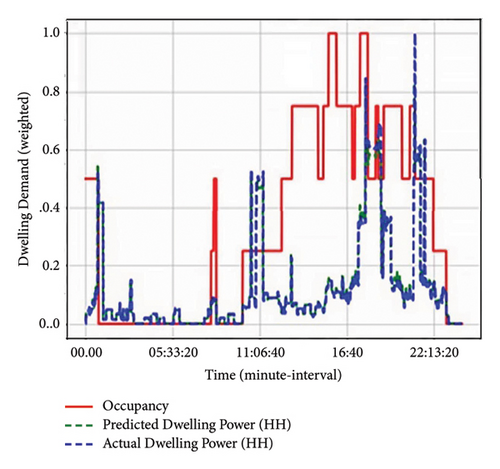
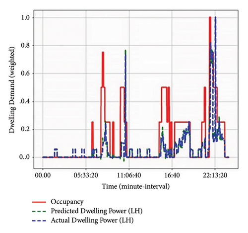
The obtained results with respect to energy usage and occupancy are illustrated in Figures 3 and 4 for the emerging high-income (EH) earner group also known as low high-income earners (LH) and realized high-income (RH) earners also referred to as high high-income earners (HH), respectively. Based on the results, it can be inferred that occupants normally occupy houses during the morning and evening periods with little or no occupancy during the daytime. These results correspond to the historical survey questionnaires. This is due to the heavy loads, e.g., cooking appliances, wet appliances, space heating, and water heating that are mostly utilized during morning and evening times when household dwellers prepare to go or come back from their respective schooling/working places. Inclusive of the energy usage are the low energy consumption appliances, i.e., lighting (in the morning and evening). During such periods, the occupants tend to move from one room to another within their households. As demonstrated in Figures 3 and 4, there is a strong relationship that exists between energy usage and occupancy presence. As seen, the occupant/s behavior with respect to actions/occupants’ activities is very crucial in energy demand. The switch-on event occurrences are correlated to the occupant/s presence in the room. Based on the results shown in Figure 4, it can be seen that between 05: 33 and 11: 06, the rooms are occupied, and between 11: 06 and 16: 40, there is little to no occupancy in rooms, as represented by switch-off events (inactive occupancy). However, from 16: 40 to 22: 13, occupants occupy respective rooms or engage in activities that are synonymous with such designated space. This is as a result of occupants returning from their respective schooling/working areas (active occupancy). Such analysis was also verified by the historical data. Based on the results, occupancy presence influences energy consumption disparity and it was deduced as shown in Figure 3 that more occupants occupying a dwelling do not necessarily translate into an increase in energy usage. As can be noted between 13: 00 and 16: 40, there was high room occupancy for HH/EH group; however, less energy was consumed around such hours. This investigation has categorized occupancy profiles into six and assigned weights ranging between 0 and 1, corresponding to the proportion of time (period) when the utilization of an appliance/lighting can occur due to occupancy by person/s. These weights are demonstrated in Table 1 and they are prone to be capricious throughout the day.
| Number of occupants | Occupancy weight |
|---|---|
| Zero person | 0.00 |
| One person | 0.15 |
| Two persons | 0.30 |
| Three persons | 0.45 |
| Four persons | 0.60 |
| Five persons | 0.75 |
| Six persons | 1.00 |
3.1.2. Low-Income Group
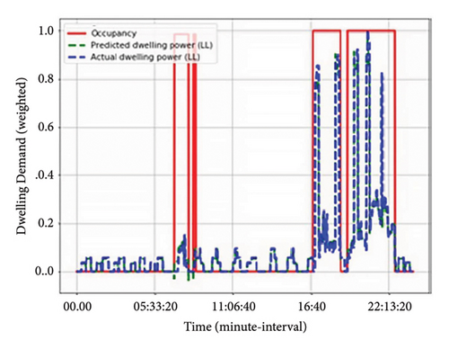
The obtained results for energy usage and occupancy are illustrated in Figures 5 and 6 for both low low-income earners (LL) and upper low-income (UL) earners, respectively. It can be noted that occupancy as per the low-income group varies, and this may have been due to incomparable lifestyles and the different job types (i.e., work-going income earners or working from home income earners). Just like with the high-income earners’ group, the switch-ON events represent occupants’ presence in the room.
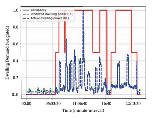
3.1.3. Middle-Income Group
Likewise, the middle-income earners’ group was investigated with respect to energy usage and occupancy. It was found that occupancy as per the middle-income group varies per income level (EM and RM) and appliance/lighting usage pattern. This may have been due to incomparable lifestyles and the different job types (i.e., work-going income earners or working from home income earners). Just like with the low and high-income earners’ group, the switch-ON events represent occupants’ presence in the room.
3.2. Occupants’ Activities
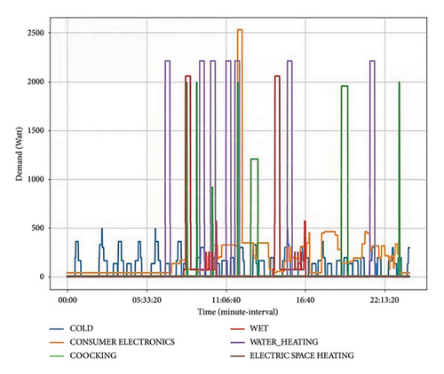
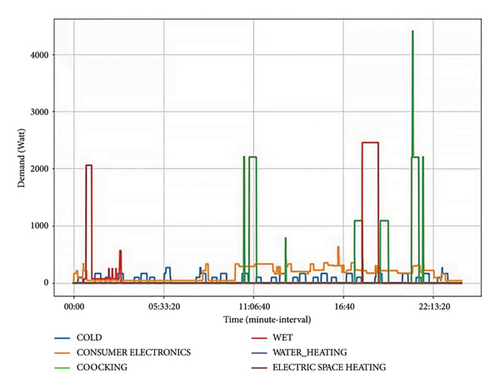
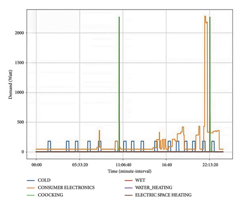
Household activities have an impact on energy usage. Household activities are grouped based on appliances utilized by occupants to perform activities. For example, cooking appliances consist of appliances such as a kettle, microwave, hob, and oven. Under cooking appliances, any of the mentioned appliances may be ON during a specific period or time-of-use. Weights are used to distinguish the active appliance/s (Pappliance) as represented by different power ranges, where Pu ≠ Pv ≠ Pw ≠ Px ≠ Py ≠ Pz as demonstrated in Table 2. The actual energy usage based on activities is illustrated in Figures 7, 8, and 9 for high, middle, and low-income earners, respectively.
| Activities | Appliance power (W) | Weight |
|---|---|---|
| No appliance utilized (Pu) | 0 | 0 |
| Very low energy consumption appliances (Pv) | 1–99 | 0.2 |
| Low energy-consuming appliances (Pw) | 100–300 | 0.4 |
| Medium energy-consuming appliances (Px) | 400–900 | 0.6 |
| High energy-consuming appliances (Py) | 1000–1400 | 0.8 |
| Very high energy-consuming appliances (Pz) | 1500–4000 | 1.0 |
3.3. Income
- (i)
Low low-income earner (LL) class: 3 rooms or less
- (ii)
Upper low-income earner (UL) class: 4 rooms or more than 4
- (iii)
Emerging middle-income earners (EM): a maximum of 6 rooms
- (iv)
Realized middle-income earners (RM): 7 rooms or more
- (v)
Emerging high-income earners (EH)/low high-income earners (LH): a maximum of 10 rooms
- (vi)
Realized high-income earners (RH)/high high-income earners (HH): 11 rooms or more
Each income class was allocated a weight to distinguish it from other income classes as follows: LL-0.166; UL-0.332; EM-0.498; RM-0.664; EH/LH-0.830; and RH/HH-1.000.
4. Simulation Outputs
The train-validation-test datasets were separated into 70%, 15%, and 15%, respectively. The model was further trained by loading the training data into the ANN graphic user interface (GUI) from MATLAB workspaces. The gradient descent method was employed in this study, as an ordinary backpropagation learning algorithm together with the Levenberg–Marquardt algorithm for training a feed-forward network. Throughout the training process, an input-output mapping was created by the network, and the weights and biases were adjusted to minimize the produced output error till the targeted output was achieved. Based on the obtained error from the output layer, the error is backpropagated through the network enabling the adjustment of the neurons’ weights and threshold values, to reduce the error in the next iteration [21]. The output layer consists of one neuron as a representative of the output variable being the total demand value. On completion of the network training process, the prediction outputs of the ANN-based model are demonstrated in Tables 3, 4, 5, 6, 7, and 8 per income level. Also, to evaluate the model’s performance accuracy, some statistical analyses were used per income level (EM, RM, HH, LH, LL, and UL, respectively).
| Time, GMT + 01: 00 | Input | Output | ||
|---|---|---|---|---|
| Income level/weight-EM | Active occupancy | Total dwelling appliance usage | ANN-based output | |
| 02: 30: 00 | 0.498 | 0 | 0.052287215 | 0.06264922 |
| 05: 00: 00 | 0.498 | 0.15 | 0.060829793 | 0.074883255 |
| 06: 00: 00 | 0.498 | 0.60 | 0.029393307 | 0.029624214 |
| 16: 00: 00 | 0.498 | 0.30 | 0.063916661 | 0.037970025 |
| 20: 00: 00 | 0.498 | 1 | 0.158565135 | 0.147527939 |
| 21: 00: 00 | 0.498 | 0.75 | 0.186823155 | 0.205742271 |
| 23: 30: 00 | 0.498 | 0 | 0.003331833 | 0.00644806 |
| Time, GMT + 01: 00 | Input | Output | ||
|---|---|---|---|---|
| Income level/weight-RM | Active occupancy | Total dwelling appliance usage | ANN-based output | |
| 00: 00: 00 | 0.664 | 0 | 0.00152975 | 0.001608746 |
| 04: 00: 00 | 0.664 | 0.15 | 0.044084529 | 0.0482291121 |
| 10: 00: 00 | 0.664 | 0.60 | 0.086107608 | 0.075346084 |
| 18: 30: 00 | 0.664 | 1 | 0.933396596 | 0.921076683 |
| 21: 00: 00 | 0.664 | 1 | 0.849660966 | 0.860230713 |
| 21: 30: 00 | 0.664 | 0.30 | 0.174076839 | 0.182890749 |
| 23: 00: 00 | 0.664 | 0 | 0.058800702 | 0.045092318 |
| Time, GMT + 01: 00 | Input | Output | ||
|---|---|---|---|---|
| Income level/weight-HH | Active occupancy | Total dwelling appliance usage | ANN-based output | |
| 01: 30: 00 | 1 | 0 | 0.048810250 | 0.042414582 |
| 02: 00: 00 | 1 | 0.15 | 0.034980679 | 0.030433611 |
| 08: 00: 00 | 1 | 0.15 | 0.077282896 | 0.078396274 |
| 17: 00: 00 | 1 | 0.60 | 0.135245068 | 0.160734906 |
| 19: 00: 00 | 1 | 1 | 0.387227984 | 0.387437314 |
| 21: 30: 00 | 1 | 0.45 | 0.134838316 | 0.146613894 |
| 22: 30: 00 | 1 | 0 | 0.055318283 | 0.062042771 |
| Time, GMT + 01: 00 | Input | Output | ||
|---|---|---|---|---|
| Income level/weight-LH | Active occupancy | Total dwelling appliance usage | ANN-based output | |
| 05: 30: 00 | 0.830 | 0.30 | 0.380729112 | 0.382415873 |
| 07: 30: 00 | 0.830 | 0.15 | 0.007086941 | 0.006942033 |
| 17: 30: 00 | 0.830 | 0.60 | 0.092820181 | 0.082415579 |
| 19: 00: 00 | 0.830 | 1 | 0.140038809 | 0.124848206 |
| 21: 30: 00 | 0.830 | 0.75 | 0.185640362 | 0.194924760 |
| 22: 30: 00 | 0.830 | 0.15 | 0 | 0 |
| 23: 30: 00 | 0.830 | 0 | 0 | 0 |
| Time, GMT + 01: 00 | Input | Output | ||
|---|---|---|---|---|
| Income level/weight-LL | Active occupancy | Total dwelling appliance usage | ANN-based output | |
| 00: 00: 00 | 0.166 | 0 | 0 | 0 |
| 04: 30: 00 | 0.166 | 0.15 | 0.058558558 | 0.053547842 |
| 06: 00: 00 | 0.166 | 0.75 | 0.058558558 | 0.053547842 |
| 06: 30: 00 | 0.166 | 1 | 0 | 0 |
| 16: 00: 00 | 0.166 | 0.45 | 0 | 0 |
| 20: 30: 00 | 0.166 | 1 | 0.113577863 | 0.1224899289 |
| 23: 00: 00 | 0.166 | 0 | 0.005855855 | 0.005354784 |
| Time, GMT + 01: 00 | Input | Output | ||
|---|---|---|---|---|
| Income level/weight-UL | Active occupancy | Total dwelling appliance usage | ANN-based output | |
| 01: 00: 00 | 0.332 | 0 | 0 | 0 |
| 04: 30: 00 | 0.332 | 0.15 | 0 | 0 |
| 06: 00: 00 | 0.332 | 1 | 0.344604952 | 0.343686531 |
| 07: 00: 00 | 0.332 | 0.60 | 0.137971981 | 0.136278341 |
| 18: 30: 00 | 0.332 | 0.75 | 0.296108490 | 0.309637894 |
| 21: 00: 00 | 0.332 | 1 | 0.133254716 | 0.135941353 |
| 22: 30: 00 | 0.332 | 0 | 0.066185141 | 0.05447203 |
4.1. Model Validation
The model’s performance validation was observed by learning the relationship between the actual measured data and the forecast outputs using the graphical plots and statistical analysis/inferences. Such technical and numerical procedures will be demonstrated in this section per income level.
4.1.1. Correlation Analysis
The correlation coefficient (r) measures the strength and direction of the linear relationship between two variables (i.e., actual (x) and predicted output (y)) [5]. The value of r is expected to range between −1 ≤ 0 ≥ +1. The signs − and + denote negative and positive correlations, respectively. A negative correlation shows that as the value of x increases, y also decreases. However, for positive correlation, the relationship is denoted by an increase in values of x results to increase in y values. For this analysis, the r-values were deduced using (9). This can also be validated by finding the square root of R2 as stated in (10). R2 known as coefficient of determination or goodness of fit determines the “strength of certainty of prediction” [5]. The deductions made from using randomly selected data for low, middle, and high-income earners applying (9) and (10) are demonstrated in Table 9 (see Appendix B).
| Income class | Pearson’s coefficient correlation (r) | Coefficient of determination (R2) |
|---|---|---|
| EM | 0.8310 | 0.6905 |
| RM | 0.8401 | 0.7058 |
| HH/RH | 0.9936 | 0.9872 |
| LH/EH | 0.9983 | 0.9966 |
| LL | 0.9817 | 0.9767 |
| UL | 0.9452 | 0.8934 |
Based on these results, the proposed developed model demonstrated a good relationship and a positive fit. The r-values show strong positive correlation as defined by Schober et al. [22] in their study of correlation coefficient interpretation.
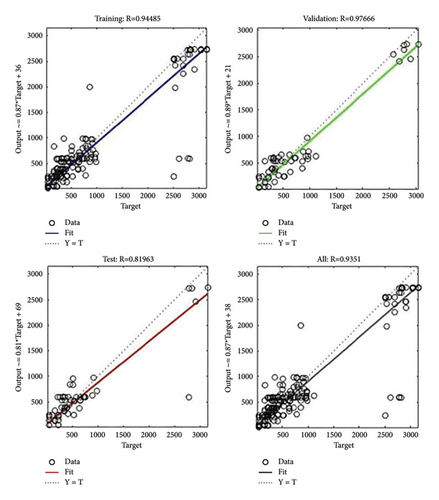
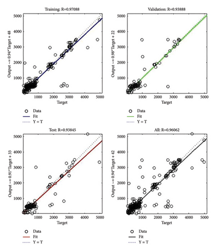
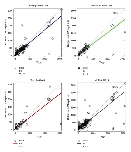
To further determine the strength of the linear relationship between the actual and predicted outputs, the regression analysis for the ANN training, validation, and testing, respectively, per income level, LL, HH, and EM, is shown in Figures 10, 11, and 12.
4.1.2. The Regression Model
For additional validation, the model’s reliability was analyzed per income level.
(1) Low Income. This was carried out based on the technical and numerical procedures, using randomly selected minute interval predicted output values for both low low-income and the upper low-income group. Based on the obtained results, the ANN-based model predicted very well with high R2 values per income earners groups. The R2 values for low low-income earners are as follows: 0.9637, 0.9428, 0.9432, 1.000, and 0.9704, while the R2 values for upper low-income earners are as follows: 0.8934, 0.8316, 0.6987, 0.9704, and 0.7841. The root mean square error values for low low-income earners are as follows: 0.0349, 0.0362, 0.0687, 0.0391, and 0.0492, while those for upper low-income earners are 0.0072, 0.0383, 0.0324, 0.037, and 0.0109, respectively. The FFNN model computational time is better reduced while fewer neurons in the hidden layer are used for better accuracy. To discover the impact of the FFNN structure on prediction accuracy, the performance of various neuron sizes was investigated. Firstly, the three-layer FFNN model was investigated with 10 neurons in the hidden layer till 160 neurons were used. During the training process, the network creates an input-output mapping, and the weights and biases are adjusted to reduce the produced output error until the desired/acceptable output is achieved. At this stage, the network can result in accidental samples showing false performance measures. Hence, it is crucial to retrain the network at least ten times, instead of considering the “so-called” good performance indices that could be achieved straightaway to evaluate the robustness of the performance. The retraining was done to eradicate the ramifications of the randomness of the initial setting of weights and bias on the prediction accuracy. Based on the obtained error from the output layer, the error was backpropagated through the network enabling the adjustment of the neurons’ weights and threshold values, to reduce the error in the next iteration. This process was repeated until a satisfactory prediction result (acceptable output) was attained. The outputs were considered to be satisfactory/acceptable based on the MAPE values; the lower the MAPE, the more accurate the forecast model. The benchmark for the accuracy of the model based on the MAPE evaluation was developed by Lewis [22] and is demonstrated in Table 10.
| MAPE | Interpretation |
|---|---|
| ≥10 | Highly accurate forecasting |
| 10 ≥ 20 | Good forecasting |
| 20 ≥ 50 | Reasonable forecasting |
| >50 | Inaccurate forecasting |
Based on the one-minute interval outputs, the mean absolute percentage error values for low low-income earners are as follows: 1.77%, 1.36%, 2.28%, 1.54%, and 1.81%, whereas those for the upper low-income earners are 0.75%, 1.4%, 0.85%, 1.09%, and 1.24% compared to the real value output, which indicates a high accuracy. Based on these results, the upper low-income group outperformed the low low-income group, yielding a low error varying from 0.75% to 1.4% (MAPE), while the MAPE of the low low-income group varies from 1.36% to 2.28%. The lowest MAPE is achieved when 120 neurons in the hidden layer are applied, and this hidden-neuron size is viewed as the best configuration of this model. Based on MAPE values, it can be concluded that the ANN-based model has forecasted with high accuracy since the MAPE values are all below 10 which translates into highly accurate forecasting.
(2) High Income. Likewise, the model’s reliability in contrast with the actual values was observed for both low high-income earners and high high-income earners using randomly selected minute interval predicted output values. The ANN-based model forecasts accurately with high values of R2. The R2 values for low high-income earners are as follows: 0.9966, 1.0000, 0.7518, 0.7889, and 0.7542, whereas the R2 values for high high-income earners are as follows: 0.9872, 1.0000, 1.0000, 0.7017, and 0.6613, respectively. The root mean square error values for low high-income earners are as follows: 0.0356, 0.0044, 0.0402, 0.005, and 0.0052, while those for high high-income earners are 0.01437, 0.0351, 0.0159, 0.04, and 0.0366, respectively. The root mean square error level for low high-income earners is lower than that of high high-income earners as the LH group ranges from 0.005 to 0.0402 while the HH group ranges from 0.01437 to 0.04. Based on the one-minute interval outputs, the mean absolute percentage error values for low high-income earners are as follows: 2.69%, 0.16%, 1.36%, 0.16%, and 0.17%, whereas those for the high high-income earners are 1.21%, 1.29%, 0.61%, 1.25%, and 1.13% compared to the real value output, which indicates a high accuracy. Similar to the low-income grouping, based on the obtained results, the high high-income group outperformed the low high-income group, yielding a low error varying from 0.61% to 1.25% (MAPE), while the MAPE of the low high-income group varies from 0.16% to 2.69%. Going by the MAPE values, it can be concluded that the ANN-based model has forecasted with high accuracy.
(3) Middle Income. The model’s reliability in contrast with the actual values was observed for both emerging middle-income earners (EM) and realized middle-income earners (RM) using randomly selected minute interval predicted output values. The ANN-based model estimated accurately with good values of R2. The R2 values for emerging middle-income earners are as follows: 0.6903, 0.6111, 0.6514, 0.6969, and 0.7014, whereas the R2 values for realized middle-income earners are as follows: 0.7058, 0.5804, 0.6191, 0.5535, and 0.7313, respectively. The root mean square error values for emerging middle-income earners are as follows: 0.0238, 0.0156, 0.0042, 0.0076, and 0.0936, while those for realized middle-income earners are 0.0085, 0.0148, 0.0062, 0.0196, and 0.0071, respectively. The root mean square error level for emerging middle-income earners is higher than that of realized middle-income earners as the EM group ranges from 0.0042 to 0.0238 while EM group ranges from 0.0062 to 0.0196. Based on the one-minute interval outputs, the mean absolute percentage error values for emerging middle-income earners are as follows: 1.71%, 1.09%, 2.08%, 0.06%, and 2.55%, whereas those for the realized middle-income earners are 0.67%, 0.79%, 0.82%, 0.02%, and 1.47% compared to the real value output, which indicates good accuracy. Based on these results, the realized middle-income group outperformed the emerging middle-income group, yielding a low error varying from 0.02% to 1.47% (MAPE), while the MAPE of the emerging middle-income group varies from 0.06% to 2.55%. As indicated by the MAPE values, it can be concluded that the ANN-based model forecasted with good accuracy.
5. Trend Analysis and Demand Computation
5.1. Trend Analysis
The trend analysis was also carried out per income level to spot a pattern from each income earner’s predictor TOU outputs to the actual output.
5.1.1. High-Income Earners
The ANN-based model demonstrated better accuracy with respect to the actual output. The household usage pattern per income (for both EH and RH) levels for time series analysis is shown in Figures 13 and 14.
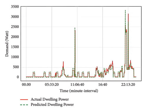
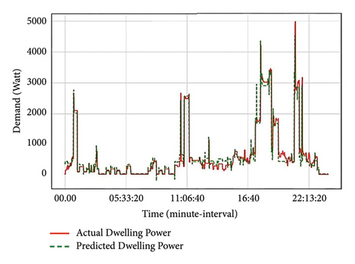
As exhibited in these figures, income earnings have a substantial impact on energy usage output. From the results, RH earners are more comfortable and do not pay much attention to their energy usage. Both groups start their day around 5: 33: 20 as they utilize the water heater for bathing purposes and from that period their consumption slightly decreases. However, the demand for RH group gradually rises again from 11: 06: 40, whereas the EH group is more conservative in their energy usage during this period, unlike the RH groups. This rise in demand in RH group is due to occupants performing various activities within a household at such periods as illustrated in Figure 8. Again from 16: 40, both EH and RH groups have a sudden increase in demand as occupants return from their respective workplaces. However, the RH group’s demand based on the predictor is higher than EH demand.
5.1.2. Low-Income Earners
Figures 15 and 16 show the profiles for low-income earners (both LL and UL).
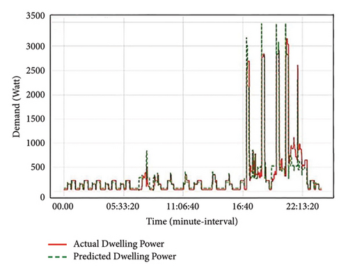
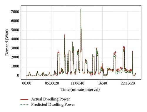
Based on the results, it can be seen that income earnings affect energy usage. There is an abrupt rise in the energy output (load) mostly experienced by UL group from 5: 33: 20 which is a bit higher than that of the LL group during morning standard and peak hours. However, the LL group mostly experiences a sudden rise during evening peak hours. Going by the results, it can be seen that profiles for the low-income earners differ; this may be due to different occupations within the groupings. The LL earners’ households were mostly unoccupied from 07: 00, and this may be due to occupants heading to their respective workplaces. As a result of unoccupied periods, there is a sudden decrease in energy usage from that time up until 16: 40 as occupants return to their respective homes. Also, this can be due to occupants available in their home but performing non-energy-related activities, and LL-income class lacks a variety of appliances, unlike the UL-income class. A steady rise is experienced after 16: 40 as the LL group arrives at their respective homes and engages in energy-related activities (appliances/lighting usage). Such appliances utilized include the use of cooking appliances, consumer electronics, and lighting. After 22: 13: 20, a sudden decrease in energy usage is experienced by the LL class; this can be as a result of the LL group going to bed. On the contrary, the UL group experienced a sudden decrease after 23: 00 to 5: 33: 20, unlike LL grouping.
(1) Demand Analysis. The demand analysis was also carried out and the developed model provided a good depiction of the morning standard/peak time of use together with the evening peak time of use periods as demonstrated in Figures 17, 18, 19, 20, 21, and 22 per income level.
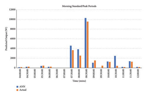
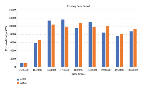
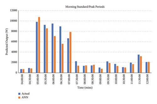
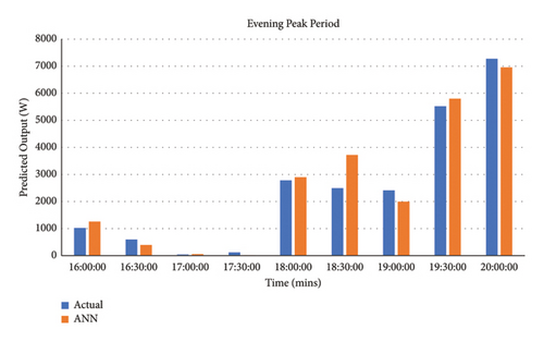
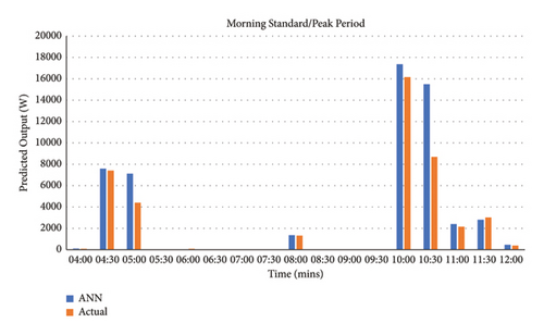
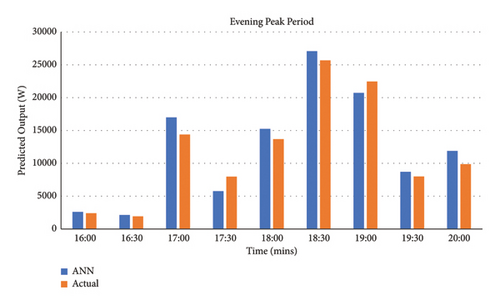
The MAPE results for the demand were deduced using (8) per income group (evening peak TOU periods were deduced between 16: 00 and 20: 00 and morning standard TOU periods from 09: 00 to 12: 00, whereas the morning peak TOU periods were deduced between 04: 00 and 08: 00). Table 11 shows the MAPE values for the demand during the evening peak, morning standard, and morning peak TOU periods per income level in contrast with the real output. These MAPE values prove highly accurate forecasting; the scale of interpretation for prediction accuracy is demonstrated in Table 11.
| Category | Low-income (%) | Middle-income (%) | High-income (%) |
|---|---|---|---|
| Evening peak | 0.061 | 0.398 | 0.474 |
| Morning standard | 3.755 | 1.659 | 3.005 |
| Morning peak | 2.489 | 1.167 | 1.989 |
These MAPE values prove highly accurate forecasting; the scale of interpretation for prediction accuracy is demonstrated in Table 10.
6. Comparative Study of the Proposed Technique
Comparative performance study of the proposed model with two existing models (Sections 6.1 and 6.2) not having interlinked household behavior variables as inputs was undertaken. The comparative study is expected to bring into perspective occupancy interpretation, its dependence, and impact quantification in relation to load profile development. The income level focus of the study is the low-income group.
6.1. Modelling the Residential Buildings’ Electrical Energy Consumption Profile in Iran [23]
Sepehr et al.’s investigation [24] deduced that the more the occupants, the larger the random behaviors, thereby translating to high demand peaks. In the study, to ascertain the impact of household energy consumption, the authors developed a bottom-up method using a one-minute time interval and two influential factors, namely, the number of occupants (occupancy) and how occupants interact with various appliances. The key concept was to determine the probability of switching on appliances and addition of all kinds of consumption to determine the household total energy consumption.
The domestic energy consumption model developed is established on the energy consumption hours and the product of the nominal power and frequency of the domestic appliances. Whenever an appliance is turned ON, the nominal power of the appliance is measured during the operational cycle (a crucial part of the study).
| House category | No. of inhabitants (occupancy) | Frequency |
|---|---|---|
| A single adult having no kid(s) or a single retired adult | 1 | 0.2 |
| A single adult having a kid or 2 adults having no kids or 2 retired adults | 2 | 0.24 |
| 2 adults and a child or 3 adults | 3 | 0.19 |
| 2 adults having 2 kids or 3 adults and a child or 4 adults | 4 | 0.28 |
| 2 adults with 3 or more kids or 3 adults with 2 or more kids | ≥5 | 0.19 |
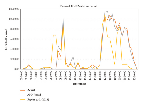
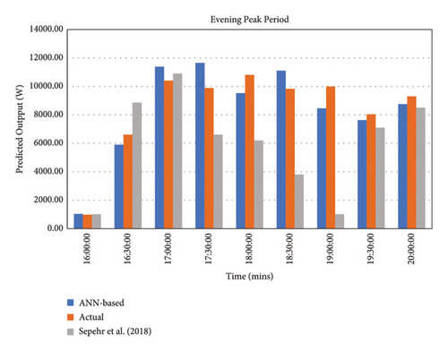
The various appliances per household were assigned nominal power, their standby power, along with the duration of their operational cycle. For low-income households, a 24-hour 30-minute time resolution simulation was carried out using Table 13. The simulated energy profile for the low-income earner group is illustrated in Figure 23, while Figure 24 represents the demand output during the night peak period. The demand MAPE of these models in contrast to the actual demand is demonstrated in Table 14.
| Time, GMT + 01: 00 | ANN-based | Actual | Sepehr et al. [24] | Behm et al. [25] |
|---|---|---|---|---|
| 00: 00: 00 | 0 | 0 | 0 | 104.218 |
| 00: 30: 00 | 140.15072 | 190.7336 | 233 | 109.325 |
| 01: 00: 00 | 232.816865 | 304.5045 | 345 | 124.831 |
| 01: 30: 00 | 788.095141 | 950 | 1009 | 693.628 |
| 02: 00: 00 | 232.81686 | 304.5045 | 345 | 104.853 |
| 02: 30: 00 | 0 | 0 | 0 | 260.943 |
| 03: 00: 00 | 0 | 0 | 0 | 138.028 |
| 03: 30: 00 | 0 | 0 | 0 | 52.390 |
| 04: 00: 00 | 140.15072 | 159.4764 | 173 | 104.39 |
| 04: 30: 00 | 232.81686 | 254.6026 | 310 | 104.390 |
| 05: 00: 00 | 0 | 0 | 310 | 521.950 |
| 05: 30: 00 | 414.235806 | 471.3555 | 310 | 1393.804 |
| 06: 00: 00 | 232.81686 | 254.6026 | 310 | 4997.980 |
| 06: 30: 00 | 0 | 0 | 6800 | 5644.181 |
| 07: 00: 00 | 0 | 0 | 6800 | 5473.747 |
| 07: 30: 00 | 4584.05704 | 3659.588 | 1850 | 6403.909 |
| 08: 00: 00 | 3843.5686 | 2530.893 | 1850 | 4567.500 |
| 08: 30: 00 | 10281.4736 | 9546.495 | 9010 | 4939.733 |
| 09: 00: 00 | 1064.4805 | 1533.205 | 1000 | 6756.341 |
| 09: 30: 00 | 496 | 462.7523 | 520 | 6621.061 |
| 10: 00: 00 | 1324 | 1229.612 | 1003 | 6644.825 |
| 10: 30: 00 | 2476 | 428.1938 | 500 | 3714.000 |
| 11: 00: 00 | 208 | 173.9132 | 160 | 1565.85 |
| 11: 30: 00 | 1376 | 1272.515 | 1500 | 460.387 |
| 12: 00: 00 | 208 | 173.9132 | 195 | 104.390 |
| 12: 30: 00 | 208 | 173.9132 | 360 | 104.390 |
| 13: 00: 00 | 208 | 173.9132 | 183 | 104.390 |
| 13: 30: 00 | 208 | 173.9132 | 183 | 104.390 |
| 14: 00: 00 | 548 | 514.0256 | 550 | 321.265 |
| 14: 30: 00 | 208 | 903.4145 | 450 | 121.940 |
| 15: 00: 00 | 548 | 514.0256 | 0 | 321.265 |
| 15: 30: 00 | 208 | 173.9132 | 233 | 121.940 |
| 16: 00: 00 | 1036 | 977.9478 | 1010 | 518.000 |
| 16: 30: 00 | 5892.08325 | 6604.505 | 8860 | 1219.400 |
| 17: 00: 00 | 11379.3324 | 10406.85 | 10900 | 7480.550 |
| 17: 30: 00 | 11646.26 | 9879.59 | 6600 | 8576.838 |
| 18: 00: 00 | 9515.46497 | 10806.57 | 6200 | 5848.562 |
| 18: 30: 00 | 11098.4155 | 9827.622 | 3800 | 9218.664 |
| 19: 00: 00 | 8450.40136 | 9985.405 | 1010 | 12567.324 |
| 19: 30: 00 | 7632.74806 | 8039.189 | 7090 | 8975.800 |
| 20: 00: 00 | 8753.16417 | 9291.248 | 8500 | 8908.865 |
| 20: 30: 00 | 6527.66328 | 6463.063 | 1000 | 4829.028 |
| 21: 00: 00 | 8326.60752 | 8258.687 | 1000 | 1993.580 |
| 21: 30: 00 | 7558.46131 | 8169.884 | 1000 | 1231.105 |
| 22: 00: 00 | 4610.57007 | 4872.973 | 315 | 618.310 |
| 22: 30: 00 | 2601.86597 | 3873.555 | 127 | 1283.555 |
| 23: 00: 00 | 1309.17512 | 1516.667 | 0 | 519.943 |
| 23: 30: 00 | 140.15072 | 190.7336 | 0 | 104.390 |
| MAPE (low-income) | |
|---|---|
| Model | Evening peak period (%) |
| ANN-based model | 0.061 |
| Bottom-up method | 3.202 |
Equation (8) was applied in the determination of the MAPE result. Using selected TOU values from Table 13, evening peak TOU periods were deduced between 16: 00 and 20: 00. Based on the MAPE result obtained, the ANN-based model outperformed the Sepehr et al. [24] technique, i.e., bottom-up approach.
According to the obtained outcomes/results, the number of inhabitants in the dwelling is correlated to the behavioral pattern; the energy consumption per occupant as applied in Sepehr et al. [24] seems inaccurate in relation to occupancy utilization. Observations show that the lighting estimation yielded inaccurate prediction results in most cases using the bottom-up approach. This was due to the lighting being found to be active almost every time/hour of the day, thereby providing an unrealistic performance of dwellers’ utilization; also, the lighting wattage rating breakdown for each room of the house was not considered in terms of calculation/estimation. The actual daily average consumption is 4.614 kWh, while the monthly consumption is 138.406 kWh and the annual energy consumption is 1660.876 kWh. The estimation arising from the models (i.e., ANN and Sepehr et al. [24]) is stated in Table 15.
| Comparison of energy consumption (low-income) | |||
|---|---|---|---|
| Category | Actual (kWh) | ANN (kWh) | Satre-Meloy [11] (kWh) |
| Daily | 4.614 | 4.654 | 3.193 |
| Monthly | 138.406 | 139.627 | 95.782 |
| Annually | 1660.876 | 1675.527 | 1149.385 |
Based on certain intervals arising from the model’s application at time-of-use periods, e.g., 16: 00: 19: 00, a high error disparity is seen with the Sepehr et al. [24] model and the actual data-graphical representation. This may be due to the increase in occupant activity and their various impulsive behaviors arising from the shortcomings of the model [24]. It can be inferred that the more the occupants’ random behaviors, the greater the inaccuracy in various existing model prediction as demonstrated by the models’ estimation outputs and the high MAPE value. This invariably supports the need for interlinked behavioral variables in model development.
6.2. Modelling European Electricity Load Profiles Using an Artificial Neural Network Method [24]
Behm et al.’s study [25] entailed the use of an artificial neural network to generate weather-dependent, energy load profiles for European countries using 60-minute intervals. In the work, annual peak load and weather data were used as input parameters. Influential factors such as direct irradiance, outdoor temperature, diffuse irradiance, and wind speed were considered in the generation of the weather data. The authors are of the opinion that both cloudiness and humidity have an impact on weather. However, data for both parameters (cloudiness and humidity) were not available during the study period, although the authors believed that they could be deduced from the ratio of the irradiances. The load and the weather data from the year 2006 to 2016 (over ten years) were applied. Table 16 shows the input parameters of Behm et al.’s study [25].
| No | Characteristic input | Value range |
|---|---|---|
| 1 | Yearly peak load (MW) | 72.974–79.884 |
| 2 | Temperature (°C) | −16.38–34.30 |
| 3 | Wind speed (ms−1) | 0–17.64 |
| 4 | Direct irradiance (Wm−2) | 0–845.66 |
| 5 | Diffuse irradiance (Wm−2) | 0–397.83 |
Given the fact that the proposed model is computational intelligence-based, it will be very enlightening and insightful to compare the proposed study (ANN-based model using low income) with another ANN-based model that is not based on occupancy and interactions or activities in residential buildings. The Behm et al. [25] model is comparable to this current study, although the methodology (approach) and variables used differ. Since most of the input variables used in the Behm et al. [25] model are not unavailable, the demand profile was developed using only the irradiance model, that is, ANN 2 model. The irradiance data used were weighted as illustrated in Table 17.
| Irradiance level | Weight | Time |
|---|---|---|
| No natural lighting | 0 | 00: 00–05: 30 |
| Medium natural lighting (diffuse irradiance) | 0.5 | 05: 31–08: 00 |
| High natural lighting (direct irradiance) | 0.75 | 08: 01–10: 30 |
| Very high natural lighting (direct high irradiance) | 1 | 10: 31–17: 29 |
| Low natural lighting (direct normal irradiance) | 0.25 | 17: 30–17: 59 |
| No natural lighting | 0 | 18: 00–23: 59 |
A comparative analysis of the two models’ results was undertaken based on their expected adaptive accuracy and input parameters associated with energy consumption. The efficacy of the models was based on estimation of the two weighted ANN-based models’ electrical load profile prediction. To determine the impact of weather as applied in Behm et al. [25] and other studies, a trend analysis was carried out for the ANN 2 model. The prediction TOU outputs “with” and “without” irradiance input for the model are shown in Figure 25. It can be noted from the graphical result that indeed irradiance influences energy usage; however, irradiance being applied wholly (without income, activities, and occupancy) is not sufficient/adequate to bring about good energy consumption estimation in residential buildings (using 30-minute interval).
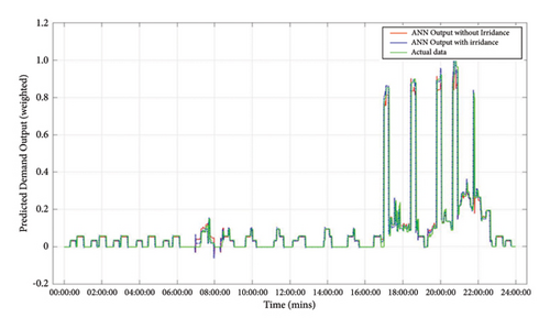
Figure 26 depicts the average daily demand profile for ANN 1 (ANN model based on occupancy, income, and interactions or activities) and ANN 2 (weather-dependent ANN model).
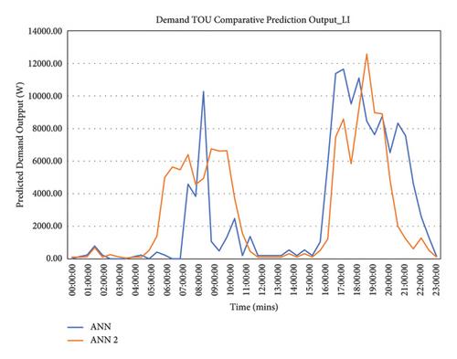
MAPE was applied to evaluate the performance and estimation prowess of both ANN-based models, and the resultant result is shown in Table 18.
| MAPE (low-income) | |||
|---|---|---|---|
| Model | Evening peak period (%) | Morning standard period (%) | Morning peak (%) |
| ANN (proposed model) | 0.061 | 3.755 | 2.489 |
| ANN (comparative model) | 1.781 | 10.336 | 7.518 |
The proposed ANN-based model showed a better accuracy outlook in comparison with the ANN model-based weather-dependent variables. The annual energy consumption for the ANN-based models to the actual energy consumption is shown in Table 19. The proposed technique was able to predict even better in comparison with ANN 2 weather-dependent method.
| Comparison of energy consumption (low-income) | |||
|---|---|---|---|
| Category | ANN 1 (kWh) | Actual (kWh) | ANN 2 (kWh) |
| Daily | 4.654 | 4.614 | 5.809 |
| Monthly | 139.628 | 138.406 | 174.29 |
| Annually | 1675.53 | 1660.876 | 2091.51 |
6.3. Comparative Inference
The proposed ANN-based technique has shown its ability to solve volatility and nonlinearity issues. The ANN-based model having characteristic inputs such as income level, household activities, and occupancy presence works better and produces accurate predictions. This can attested to by Figure 27 where the demand profiles of the various studies are compared to the actual.
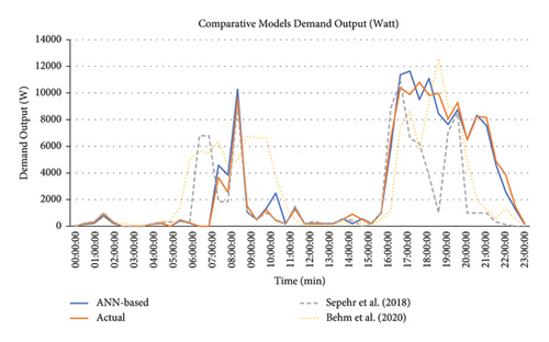
Furthermore, a summary of the findings of the comparative study in terms of the methods applied, the influential factors (variables), the yearly energy consumption, and the averaged MAPE of demand is shown in Table 20.
| Model | Method applied | Input parameters | Energy consumption/year (kWh) | MAPE (%) |
|---|---|---|---|---|
| Proposed model | ANN-based 1 | Income level, occupancy presence and activities | 1675.527 | 1.951 |
| Sepehr et al. [24] | Bottom-up method | Number of occupants and activities | 1149.385 | 3.915 |
| Behm et al. [25] | ANN-based 2 | Direct irradiance, outdoor temperature, diffuse irradiance, and wind speed | 2091.512 | 6.200 |
The proposed technique, i.e., ANN model based on occupancy and interactions or activities in residential buildings, has the ability/capacity to reduce TOU errors way better than other approaches such as the deterministic method as well as the ANN model that is based on weather variables. This thereby proves that it is a better solution/approach for energy profile development in comparison with most existing methods, including probabilistic methods.
- (i)
Assumption and inference that more occupants in relation to occupancy translate to high demand and energy utilization in residential homes, which in actual case (scenario) seems incorrect to a good degree.
- (ii)
The likelihood of switched-ON does not necessarily bring about the usage of electricity (power). The probability of such an event is mathematically intuitive. Behavior that arises from occupant activity should be learned, identified, and used for estimation. This can be extracted from historical data.
- (iii)
Weather data overreliance, e.g., direct irradiance, outdoor temperature, diffuse irradiance, wind speed, etc., without taking cognizance of actual behavior and occupancy activity and interrelated variables brings about inaccurate outcome/prediction.
7. Conclusion
This study proposed a computational intelligence model for load profile prediction in residential dwellings based on input variables, including activities and occupancy presence (interlinked variables), that influence energy usage. Based on the obtained results discussed previously in other sections, the proposed ANN-based model is inclusive of the three characteristic variables predicted (estimated) with high accuracy. The proposed model performance was attested to by the trend series analysis, demand analysis, and correlation analysis results obtained. Furthermore, a comparative study was undertaken using two existing techniques in terms of operational efficacy and the need for interlinked behavioral variables. The performance indicators—mean absolute percentage error (MAPE), mean square error (MSE), and root mean square error (RMSE)—showed good confidence levels with respect to the actual data. The ANN-based model further demonstrated its proficiency in management of extra-large and very multifaceted systems with many interrelated variables. There were also concerns that the majority of energy simulation tools are based on assumptions, thus providing a weak instrument and nonreplication of the effect occupants’ activities and occupancy on load and energy profiles in residential buildings, thereby resulting in poor energy prediction and energy demand profile. The proposed model showed its adeptness in handling such problems as demonstrated in the graphical representation of the energy usage outputs. Furthermore, the result obtained showed that applied variables, income class, occupants’ occupancy, and their interactions with households, are major determinants of energy usage estimation for profile development especially when interlinked. The ANN-based model has proven to be a more reliable and proficient tool for predicting residential energy load profiles.
The proposed model contribution validates and supports the study review undertaken by Stracqualursi et al. that the energy sector can optimize resource allocation, improve grid management, and enhance energy efficiency among others by harnessing AI [14], ultimately translating to power system reliability, reduced operational cost, and reduced environmental pollution, thereby contributing to Sustainable Development Goals 9, 11, 12 (emphasis on responsible production), and 13 [26–28].
7.1. Future Works
Having demonstrated that the developed technique is a proficient tool that can be used to achieve better prediction accuracy for energy loads, it is, therefore, necessary to look into the optimization of the ANN-based technique, i.e., the proposed model.
Conflicts of Interest
The authors declare that they have no conflicts of interest.
Acknowledgments
This work is based on the research supported wholly/in part by the National Research Foundation of South Africa (Grant No. 150574) and Tshwane University of Technology—Faculty of Engineering and Built Environment and Centre for Energy and Electrical Power. Open-access funding was enabled and organized by SANLiC Gold.
Appendix
A. Prediction Accuracy Evaluation of the Developed Models
This section describes Tables 3, 4, 5, 6, 7, 8, 21, 22, 23, 24, 25, and 26.
| Data (x and y values) | r | R2 | RMSE | MSE | MAPE (%) | |
|---|---|---|---|---|---|---|
| 1.104599484 | 1.214537887 | 0.9817 | 0.9637 | 0.0349 | 1.2169 ∗ 10−3 | 1.77 |
| 1.046205370 | 1.133644035 | 0.9710 | 0.9428 | 0.0362 | 1.3126 ∗ 10−3 | 1.36 |
| 1.118176244 | 1.271891253 | 0.9712 | 0.9432 | 0.0687 | 4.7257 ∗ 10−3 | 2.28 |
| 1.126601684 | 1.209311828 | 1.0000 | 1.000 | 0.0391 | 1.5291 ∗ 10−3 | 1.54 |
| 1.112311227 | 1.193322862 | 0.9851 | 0.9704 | 0.0492 | 2.4173 ∗ 10−3 | 1.81 |
| Data (x and y values) | r | R2 | RMSE | MSE | MAPE (%) | |
|---|---|---|---|---|---|---|
| 1.499239609 | 1.562499998 | 0.9452 | 0.8934 | 0.0072 | 5.1401 ∗ 10−5 | 0.75 |
| 1.541865677 | 1.627471915 | 0.9119 | 0.8316 | 0.0383 | 1.4657 ∗ 10−3 | 1.4 |
| 1.620876986 | 1.693326006 | 0.8359 | 0.6987 | 0.0324 | 1.0498 ∗ 10−3 | 0.85 |
| 1.43579147 | 1.518548597 | 0.9851 | 0.9704 | 0.037 | 1.3697 ∗ 10−3 | 1.09 |
| 1.460028454 | 1.556916509 | 0.8855 | 0.7841 | 0.0109 | 1.2076 ∗ 10−4 | 1.24 |
| Data (x and y values) | r | R2 | RMSE | MSE | MAPE (%) | |
|---|---|---|---|---|---|---|
| 0.510324353 | 0.589909443 | 0.9983 | 0.9966 | 0.0356 | 1.2668 ∗ 10−3 | 2.69 |
| 1.171146275 | 1.161282964 | 1.0000 | 1.0000 | 0.0044 | 1.9457 ∗ 10−5 | 0.16 |
| 1.414037242 | 1.324174122 | 0.8671 | 0.7518 | 0.0402 | 1.6151 ∗ 10−3 | 1.36 |
| 1.36919186 | 1.357999009 | 0.8882 | 0.7889 | 0.005 | 2.5056 ∗ 10−5 | 0.16 |
| 0.855776045 | 0.716214623 | 0.8685 | 0.7542 | 0.0052 | 2.7095 ∗ 10−5 | 0.17 |
| Data (x and y values) | r | R2 | RMSE | MSE | MAPE (%) | |
|---|---|---|---|---|---|---|
| 1.20416685 | 1.248118771 | 0.9936 | 0.9872 | 0.01437 | 2.0649 ∗ 10−4 | 1.21 |
| 1.13858445 | 1.217039263 | 1.0000 | 1.0000 | 0.0351 | 1.231 ∗ 10−3 | 1.29 |
| 1.20279327 | 1.167046437 | 1.0000 | 1.0000 | 0.0159 | 2.5559 ∗ 10−4 | 0.61 |
| 1.33892876 | 1.428436197 | 0.8377 | 0.7017 | 0.0400 | 1.6023 ∗ 10−3 | 1.25 |
| 0.527006671 | 0.574766248 | 0.8132 | 0.6613 | 0.0366 | 1.3376 ∗ 10−3 | 1.13 |
| Data (x and y values) | r | R2 | RMSE | MSE | MAPE (%) | |
|---|---|---|---|---|---|---|
| 1.237528375 | 1.639299612 | 0.8313 | 0.6903 | 0.0238 | 5.6859∗10−4 | 1.71 |
| 1.359416329 | 1.587821785 | 0.7818 | 0.6111 | 0.0156 | 2.4513∗10−4 | 1.09 |
| 1.317545872 | 1.561431528 | 0.8070 | 0.6514 | 0.0042 | 1.7323∗10−5 | 2.08 |
| 1.248392178 | 1.485004342 | 0.8348 | 0.6969 | 0.0076 | 5.8282∗10−5 | 0.06 |
| 1.240860208 | 1.478555162 | 0.8375 | 0.7014 | 0.0936 | 8.7647∗10−3 | 2.55 |
| Data (x and y values) | r | R2 | RMSE | MSE | MAPE (%) | |
|---|---|---|---|---|---|---|
| 1.287963713 | 1.152673432 | 0.8401 | 0.7058 | 0.0085 | 7.3587∗10−5 | 0.67 |
| 1.643272256 | 1.502106404 | 0.7618 | 0.5804 | 0.0148 | 2.2032∗10−4 | 0.79 |
| 0.337268095 | 0.32341220 | 0.7868 | 0.6191 | 0.0062 | 3.8397∗10−5 | 0.82 |
| 1.473002040 | 1.394922326 | 0.7439 | 0.5535 | 0.0196 | 3.8552∗10−4 | 0.02 |
| 1.287954062 | 1.150037841 | 0.8552 | 0.7313 | 0.0071 | 5.0766∗10−5 | 1.47 |
B. Randomly Selected Data Using Equations (8) and (9)
| x | y | xy | |
|---|---|---|---|
| 0.036679537 | 0.032234645 | 0.001182351 | |
| 0.058558559 | 0.053547843 | 0.003135684 | |
| 0.094936709 | 0.101637919 | 0.000855662 | |
| 0.801480051 | 0.879483621 | 0.704888577 | |
| 4 | 0.112944628 | 0.147633859 | 0.016677445 |
| Σ | 1.104599484 | 1.214537887 | 0.726736725 |
| 3 | 0.054550514 | 0.066740007 | 0.003640702 |
| Σ | 1.04620537 | 1.133644035 | 0.713702976 |
| 2 | 0.126521388 | 0.204987165 | 0.025935261 |
| Σ | 1.118176244 | 1.271891253 | 0.735997535 |
| 1 | 0.134946828 | 0.142407800 | 0.019217481 |
| Σ | 1.126601684 | 1.209311828 | 0.729279755 |
| 0 | 0.120656371 | 0.126418834 | 0.015253237 |
| Σ | 1.112311227 | 1.193322862 | 0.725315511 |
| x | y | xy | |
|---|---|---|---|
| 0.362478341 | 0.379716981 | 0.1376391813 | |
| 0.343256293 | 0.380454009 | 0.1305932328 | |
| 0.410413244 | 0.426444575 | 0.1750184912 | |
| 0.249625639 | 0.251474056 | 0.0627743719 | |
| 4 | 0.094254937 | 0.118826888 | 0.0112000208 |
| Σ | 1.460028454 | 1.556916509 | 0.5799996699 |
| 3 | 0.070017953 | 0.080458976 | 0.0056335728 |
| Σ | 1.43579147 | 1.518548597 | 0.51165885 |
| 2 | 0.255103469 | 0.255236385 | 0.0651116872 |
| Σ | 1.620876986 | 1.693326006 | 0.5711369644 |
| 1 | 0.17609216 | 0.189382294 | 0.0333487372 |
| Σ | 1.541865677 | 1.627471915 | 0.5393740144 |
| 0 | 0.133466092 | 0.124410377 | 0.0166045668 |
| Σ | 1.499239609 | 1.562499998 | 0.522629844 |
| x | y | xy | |
|---|---|---|---|
| 0.0297637395 | 0.034167175 | 0.001016042 | |
| 0.499085832 | 0.531218222 | 0.265123488 | |
| 0.084470251 | 0.078909904 | 0.006665539 | |
| 0.225742881 | 0.228798048 | 0.228798048 | |
| 4 | 0.527006671 | 0.574766248 | 0.302905647 |
| Σ | 1.366079375 | 1.447859597 | 0.804508764 |
| 3 | 0.499892404 | 0.555342848 | 0.2776116713 |
| Σ | 1.338928763 | 1.428436197 | 0.7792147883 |
| 2 | 0.363756915 | 0.293953088 | 0.1069274684 |
| Σ | 1.202793274 | 1.167046437 | 0.6085305854 |
| 1 | 0.299548096 | 0.343945914 | 0.1030283427 |
| Σ | 1.138584455 | 1.217039263 | 0.6046314597 |
| 0 | 0.365130491 | 0.375025422 | 0.136933216 |
| Σ | 1.20416685 | 1.248118771 | 0.638536333 |
| x | y | xy | |
|---|---|---|---|
| 0.029737395 | 0.092820181 | 0.002760230 | |
| 0.12992073 | 0.131630013 | 0.017101467 | |
| 0.164924431 | 0.163971539 | 0.010550469 | |
| 0.199149539 | 0.263232319 | 0.0524225949 | |
| 4 | 0.855776045 | 0.716214623 | 0.6129193174 |
| Σ | 1.37950814 | 1.367868675 | 0.6957540784 |
| 3 | 0.134615385 | 0.1886796 | 0.025399177 |
| Σ | 1.36919186 | 1.357999009 | 0.6722376374 |
| 2 | 0.179460767 | 0.154854713 | 0.0277903455 |
| Σ | 1.414037242 | 1.324174122 | 0.674637495 |
| 1 | 0.792345854 | 0.708178178 | 0.5611220432 |
| Σ | 1.171146275 | 1.161282964 | 0.5950454072 |
| 0 | 0.131523923 | 0.136804657 | 0.017993085 |
| Σ | 0.510324353 | 0.589909443 | 0.051912228 |
| x | y | xy | |
|---|---|---|---|
| 0.003331833 | 0.003448065 | 0.0000114884 | |
| 0.647165765 | 0.657851088 | 0.4257387026 | |
| 0.55763747 | 0.781183735 | 0.4356173216 | |
| 0.029393307 | 0.029624214 | 0.0008707536 | |
| 4 | 0.111087023 | 0.16719251 | 0.0185729182 |
| Σ | 1.237528375 | 1.639299612 | 0.8808112205 |
| 3 | 0.121887954 | 0.115714683 | 0.01410422596 |
| Σ | 1.359416329 | 1.587821785 | 0.8763424922 |
| 2 | 0.080017497 | 0.089324426 | 0.007147516989 |
| Σ | 1.317545872 | 1.561431528 | 0.8693857832 |
| 1 | 0.010863803 | 0.01289724 | 0.000140113075 |
| Σ | 1.248392178 | 1.485004342 | 0.8623783793 |
| 0 | 0.003331833 | 0.00644806 | 0.000021483859 |
| Σ | 1.240860208 | 1.478555162 | 0.8622597501 |
| x | y | xy | |
|---|---|---|---|
| 0.536567496 | 0.505465808 | 0.2712165229 | |
| 0.121900178 | 0.117779546 | 0.0143573476 | |
| 0.353903103 | 0.280849643 | 0.0993935601 | |
| 0.058800702 | 0.045092318 | 0.0026514599 | |
| 4 | 0.216792234 | 0.203486117 | 0.0441142098 |
| Σ | 1.287963713 | 1.152673432 | 0.816700531 |
| 3 | 0.572100777 | 0.552919089 | 0.3163254404 |
| Σ | 1.643272256 | 1.502106404 | 0.7039443309 |
| 2 | 0.337268095 | 0.32341220 | 0.4363064664 |
| Σ | 1.408439574 | 1.272599515 | 0.8238304863 |
| 1 | 0.401830561 | 0.445735011 | 0.4776265321 |
| Σ | 1.473002040 | 1.394922326 | 0.8652454226 |
| 0 | 0.216782583 | 0.200850526 | 0.4005762417 |
| Σ | 1.287954062 | 1.150037841 | 0.7881951322 |
Open Research
Data Availability
A 24-hour energy consumption historical data, i.e., gathered from 2008 to 2009 for 35 houses in the East Midlands, United Kingdom, was applied in the development of the models.


