Volume 2024, Issue 1 5782500
Research Article
Open Access

Chaos Control, Codimension-One and Codimension-Two 1 : 2 Strong Resonance Bifurcation Analysis of a Predator-Prey Model with Holling Types I and III Functional Responses

Abdul Qadeer Khan

Corresponding Author

Abdul Qadeer Khan

Department of Mathematics , University of Azad Jammu and Kashmir , Muzaffarabad , 13100 , Pakistan , ajku.edu.pk

Search for more papers by this author
Syeda Noor-ul-Huda Naqvi

Syeda Noor-ul-Huda Naqvi

Department of Mathematics , University of Azad Jammu and Kashmir , Muzaffarabad , 13100 , Pakistan , ajku.edu.pk

Search for more papers by this author
Shaimaa A. A. Ahmed

Shaimaa A. A. Ahmed

Department of Mathematics , College of Science and Humanities in Al-Kharj , Prince Sattam bin Abdulaziz University , Al-Kharj , 11942 , Saudi Arabia , psau.edu.sa

Department of Mathematics , Faculty of Science , Mansoura University , Mansoura , 35516 , Egypt , mans.edu.eg

Search for more papers by this author
Waleed A. I. El-Morsi

Waleed A. I. El-Morsi

Department of Mathematics , Faculty of Science , Mansoura University , Mansoura , 35516 , Egypt , mans.edu.eg

Search for more papers by this author
First published: 14 September 2024
Citations: 1
Academic Editor: Carlos Aguilar-Ibanez

Abstract

We study the existence of fixed points, local stability analysis, bifurcation sets at fixed points, codimension-one and codimension-two bifurcation analysis, and chaos control in a predator-prey model with Holling types I and III functional responses. It is proven that the model has a trivial equilibrium point for all involved parameters but interior and semitrivial equilibrium solutions under certain model parameter conditions. Furthermore, local stability at trivial, semitrivial, and interior equilibria using the theory of linear stability is investigated. We have also explored the bifurcation sets for trivial, semitrivial, and interior equilibria and proved that flip bifurcation occurs at semitrivial equilibrium. Furthermore, it is also proven that Neimark–Sacker bifurcation as well as flip bifurcation occurs at an interior equilibrium solution, and in addition, at the same equilibrium solution, we also studied codimension-two 1 : 2 strong resonance bifurcation. Then, OGY and hybrid control strategies are employed to manage chaos in the model under study, which arises from Neimark–Sacker and flip bifurcations, respectively. We have also examined the preservation of the positive solution of the understudied model. Finally, numerical simulations are given to verify the theoretical results.

1. Introduction

1.1. Motivation and Mathematical Formulation

Mathematical modeling, statistical analysis, and computational methods are all used in the interdisciplinary field of mathematical biology to investigate biological systems. Numerous subjects are covered by mathematical biology, such as genetics, ecology, epidemiology, neurology, and physiology. The interplay between prey and predator has been explained using some mathematical models. A well-known mathematical biological model that explains the dynamics of a prey-predator interaction in an ecosystem is the prey-predator model. The predator-prey interaction is a fundamental ecological relationship between two creatures in which the predator pursues, kills, and consumes the prey to survive. These interactions are extremely important in shaping the structure and functioning of ecosystems. Alfred J. Lotka and Vito Volterra separately created mathematical models to describe the dynamics of predator-prey interactions in the early twentieth century [1, 2]. The Lotka–Volterra model, commonly known as the prey-predator model, pioneered a mathematical way to analyzing these interactions. Equations in the model represent the rate of change in predator and prey populations over time, taking into consideration parameters such as predation rate, prey growth rate, and carrying capacity. It revealed details on how predator and prey populations cycle. The study of prey-predator models is still a thriving area of ecological research today. It provides a framework for understanding the dynamics of species interactions, ecosystem stability, and the effects of environmental changes on populations and communities. Scientists try to understand the complexity of predator-prey relationships and their role in changing the natural world by combining theoretical models with actual facts. It is noted that increasing evidence suggests that discrete-time prey-predator models can display a significantly wider variety of patterns compared to those observed in continuous-time models. By taking into account discrete, countable individuals rather than assuming continuous populations, discrete models enable a more accurate description of population dynamics. Choosing a discrete model for modeling the interaction between prey and predators, specifically tigers and zebras, involves several detailed considerations. First, the appeal of simplicity in these models lies in their easy to understand structure and straightforward application. In the context of periodic data collection, where information on tiger and zebra populations is gathered at regular intervals, a discrete-time model aligns neatly with the available data points. It is akin to taking snapshots at specific moments in time, providing a practical and intuitive representation of the ecological dynamics. Moreover, discrete-time models are computationally efficient, making them particularly suitable for analyses, simulations, and scenario testing. The discrete nature of these models, with updates occurring at distinct time points, lends itself to a manageable computational load, enabling researchers to explore various scenarios and model parameters efficiently. In the intricate web of predator-prey interactions, where events such as births, deaths, and predation occur discretely, a discrete-time model can capture these key moments effectively. It allows for a granular examination of population changes, mirroring the stepwise nature of ecological processes. The choice of a discrete-time framework does not imply a sacrifice of realism. Instead, it reflects a reasonable tradeoff between model simplicity and the faithful representation of essential ecological dynamics. By embracing this modeling approach, researchers gain a practical tool that not only aligns with the nature of the collected data but also enhances the manageability and interpretability of the modeling process. The discrete-time model becomes a tailored lens through which we can gain detailed insights into the nuanced interactions between tigers and zebras in their ecosystem. Many researchers investigated the discrete prey-predator models. For instance, Al-Kaff et al. [3] has investigated behavior of discrete prey-predator model as follows:
(1)
with e, a, h, b, and c are positive constants. Santra [4] has investigated behavior of the following system:
(2)
where h, ϕ, r, b, c, d, and k are positive parameters. Chakraborty et al. [5] have discussed the behavior of the following system:
(3)
with positive parameters. Chakraborty et al. [6] have explored the complex dynamics of the following discrete predator-prey model:
(4)
where h is the step size and positive model’s parameters. For further intriguing insights on this matter, we direct the reader to the work of esteemed researchers [79] and literature cited therein. Now, in order to simulate the phenomenon of predation, Holling suggested three types of functional responses for various species [10]. The Holling functional response is an ecological concept that describes how a predator’s consumption rate changes in response to shifting prey density. It has since become a key framework for understanding predator-prey interactions. The Holling functional response framework is a useful tool for studying and predicting predator-prey interactions. Researchers can capture a variety of ecological conditions and study the implications for population dynamics, stability, and coexistence by including different forms of functional responses. The functional response idea has been widely applied in ecological modeling, experimental investigations, and conservation management, helping us to better understand predator-prey interactions in natural ecosystems. In the closed first quadrant , He and Li [11] explored the behavior of discrete model with Holling type III functional response. Their model is made up of two different equations. Holling type III is used in both equations to represent the prey-predator interaction term. Saratchandran et al. [12] introduced a discrete Lotka–Volterra model to describe prey-predator interactions with Holling type I functional response. They illustrated how the predator’s survival is influenced by its natural mortality rate and the effectiveness of its predation. In this paper, we develop a discrete Lotka–Volterra prey-predator model incorporating a mixed functional response combining Holling types I and III in . So, to formulate the mathematical predator-prey model, let xt represent the prey’s density and yt represent the predator’s density. The prey-predator population evolves in accordance with the logistic map xt = axt(1 − xt), where a restricted to the interval (0, 4) represent the constant intrinsic growth rate and xt ∈ (0, 1) (see [13]). Then, the famous Lotka–Volterra model in discrete form can be written as follows:
(5)
where predator’s death rate is c(0 < c < 1). The predator-prey interaction p(xt)yt decreases the prey population, predation effectiveness is measured by the term p(xt), and the prey-predator relation q(xt)yt increases population of predator. The function q(xt) measures how a predator can use the advantage of predation to expand its population [14]. Suppose the following Holling type III functional response of a predator p(xt) (see [1518]),
(6)
where d and e denote the predation of the predator coefficient and half saturated constant, respectively. Furthermore, if q(xt) = 1 + τbxt, where τ represents the predator’s evolution rate and efficiency of predation is b(b < 1), bτxt increases the population of predator in each generation, then the required predator-prey model with Holling types I and III functional response takes the following form:
(7)
with positive initial conditions (x0, y0).

Remark 1. Discrete-time models are useful for studying different biological systems because they can show how things happen step by step. For example, in population studies, these models help understand the relationships between species, like when animals are born or die. They are also handy in genetics to see how genes change over time. When looking at cells or ecological systems, where events occur at specific times, discrete-time models are a good fit. Even in studying the brain, these models help simulate how neurons work and learn in a way that matches real-life observations. In simple terms, discrete-time models are like a helpful tool for understanding how different parts of nature change and interact.

1.2. Main Contribution

Our investigations for the model (7) in the present paper include the following:
  • (i)

    Local behavior for fixed points.

  • (ii)

    Identification of bifurcation sets for fixed points.

  • (iii)

    Analysis of codimension-one and codimension-two bifurcations in the discrete model (7).

  • (iv)

    Study of chaos by OGY and hybrid control strategies.

  • (v)

    Confirmation of theoretical results numerically.

  • (vi)

    Preservation of the positivity.

The remainder of the paper is organized as follows: Stability analysis and codimension-one bifurcation sets are discussed in Section 2 whereas codimension-one bifurcation at fixed points of the discrete model (7) is studied in Section 3. The codimension-two 1 : 2 strong resonance bifurcation analysis is studied in Section 4. The chaos control by OGY and Hybrid control strategies is presented in Section 5. To validate theoretical findings, numerical simulations are presented in Section 6. Section 7 is about the preservation of the positivity whereas future work and conclusion are given in Section 8.

2. Codimension-One Bifurcation Sets and Stability Analysis

In the present section, we explore the stability analysis at equilibrium points and codimension-one bifurcation sets for the discrete prey-predator model (7). If φ = (x, y) is an equilibrium point of (7), then one has
(8)
Since φ1 = (0, 0) and φ2 = ((a − 1/a), 0) satisfied system (8) obviously, and therefore, for all a, d, e, b, τ, and c, discrete model (7) has a trivial equilibrium φ1 = (0, 0) and a semitrivial equilibrium point φ2 = ((a − 1/a), 0) if a > 1. To get the model’s interior equilibrium point, one needs to solve the following algebraic system:
(9)
Equation (9) can also be rewritten as
(10)
and
(11)
Using (11) into (10), one gets
(12)
So, from equations (11) and (12), one can obtain that if a > (bτ/bτc), then model’s interior equilibrium point is φ3 = ((c/bτ), ((b2τ2e + c2)(bτ(a − 1) − ac)/b2cdτ2)). Now, V|φ of (7) under the map (f1, f2) ↦ (xt+1, yt+1) is
(13)
where
(14)
Hereafter, we will give local dynamics for the equilibria φ1,2,3 by the stability theory [1921]. So, for φ1, (13) becomes
(15)
with
(16)

Theorem 2. φ1 of model (7) is a

  • (i)

    sink if 0 < c < 1 and 0 < a < 1;

  • (ii)

    never source;

  • (iii)

    saddle if 0 < c < 1 and a > 1;

  • (iv)

    nonhyperbolic if a = 1.

Remark 3. Biologically, φ1 is a sink implying that predator and prey vanish, and so this case is irrelevant biologically.

Now, it is important here to note that φ1 is nonhyperbolic if a = 1. So, if a = 1 holds, then but . Finally, linked to Theorem 2, there emerges the subsequent theorem concerning the fold bifurcation set.

Theorem 4. For φ1, the fold bifurcation set is .

Now for φ2, (13) becomes
(17)
with
(18)

Theorem 5. φ2 is

  • (i)

    a sink if 1 < a < 3 and (bτ/(2 − c + bτ)) < a < (bτ/(bτc));

  • (ii)

    a source if a > 3 and a > (bτ/(2 − c + bτ));

  • (iii)

    a saddle if a > 3 and (bτ/(2 − c + bτ)) < a < (bτ/(bτc));

  • (iv)

    nonhyperbolic if a = 3 or a = (bτ/(2 − c + bτ)).

Remark 6. Biologically, it is worth noting that the stability of φ2 indicates that φ1 is unstable, which implies the presence of prey and the extinction of the predator.

It is important here to note that if φ2 is nonhyperbolic, then flip bifurcations may take place. In a more exact sense, if a = 3 holds, then but . Finally, linked to Theorem 4, there emerges the subsequent theorem concerning the flip bifurcation set.

Theorem 7. For the model’s semitrivial fixed point φ2, the flip bifurcation set is .

Now for φ3, (13) becomes
(19)
with the following characteristic equation:
(20)
that is,
(21)
where
(22)
From (21), one has
(23)
where
(24)

Theorem 8. If Δ < 0, then φ3 is a

  • (i)

    stable focus if a < (b3eτ3(c − 1) + bc2τ(c + 1)/b3eτ3(c − 1) − b2c2eτ2 + bc2τ(c + 1) − c3(2 + c)) with e >  max{(c2(c + 1)/b2τ2(1 − c)), (c2(c(2 + c) − bτ(c + 1))/b2τ2(bτ(c − 1) − c2))};

  • (ii)

    unstable focus if a > (b3eτ3(c − 1) + bc2τ(c + 1)/b3eτ3(c − 1) − b2c2eτ2 + bc2τ(c + 1) − c3(2 + c));

  • (iii)

    nonhyperbolic if a = (b3eτ3(c − 1) + bc2τ(c + 1)/b3eτ3(c − 1) − b2c2eτ2 + bc2τ(c + 1) − c3(2 + c)).

Theorem 9. If Δ ≥ 0, then φ3 is a

  • (i)

    stable node if bτ/(bτc) < a < (b3eτ3(c − 6) + bc2τ(c − 2)/b3eτ3(c − 2) − b2c2eτ2 + bc2τ(c + 2) − c3(4 + c)) with b > (c/τ) and e >  max{(c2(2 − c)/b2c2(c − 6)), (c2(c(4 + c) − bτ(c + 2))/b2τ2(bτ(c − 2) − c2))};

  • (ii)

    an unstable node if a > (b3eτ3(c − 6) + bc2τ(c − 2)/b3eτ3(c − 2) − b2c2eτ2 + bc2τ(c + 2) − c3(4 + c));

  • (iii)

    nonhyperbolic if a = (b3eτ3(c − 6) + bc2τ(c − 2)/b3eτ3(c − 2) − b2c2eτ2 + bc2τ(c + 2) − c3(4 + c)).

It is important here to note that if a = (b3eτ3(c − 1) + bc2τ(c + 1)/b3eτ3(c − 1) − b2c2eτ2 + bc2τ(c + 1) − c3(2 + c)) holds, then evaluated at φ3 has complex eigenvalues with . On the other hand, if a = (b3eτ3(c − 6) + bc2τ(c − 2)/b3eτ3(c − 2) − b2c2eτ2 + bc2τ(c + 2) − c3(4 + c)) holds, then but . Finally, linked to Theorems 8 and 9, we have the following.

Theorem 10. For the model’s interior equilibrium point φ3, the Neimark–sacker and flip bifurcation sets, respectively, are

  • (i)

    ;

  • (ii)

    .

3. Codimension-One Bifurcations

3.1. Analysis of a Flip Bifurcation for the Semitrivial Fixed Point

Based on the local dynamic study for semitrivial fixed point φ2 in Section 2, here we investigate flip bifurcation by the bifurcation theory [6, 2230]. In fact, we only have to consider the flip bifurcation when (a, d, e, b, τ, c) vary around the bifurcation set . For φ2, model (7) is invariant under y = 0, and so
(25)
From (25), one has
(26)
Finally, if x = x = ((a − 1)/a) and a = a = 3, then from (26), one gets
(27)
(28)
and
(29)

From (27)–(29), one can conclude that the flip bifurcation takes place. Based on the analysis, one has the following.

Theorem 11. Flip bifurcation takes place in (7) if .

3.2. Analysis of a Neimark–Sacker Bifurcation for the Interior Fixed Point

Based on the local dynamic study for the equilibrium φ3 in Section 2, we investigate the Neimark–Sacker bifurcation if , where a is regarded as a bifurcation parameter. So, the perturbation system of (7) becomes
(30)
where a = a + ϵ and 0 < |a| ≪ 1. It is easy to verify that perturbation system (30) has interior equilibrium φ3. For the perturbation system (30), the roots of are
(31)
where one has Λ1(ϵ) = 1 + (a + ϵ) − (2(a + ϵ)c/bτ) − (2beτ(bτ((a + ϵ) − 1) − (a + ϵ)c)/c2 + b2eτ2) and Λ2(ϵ) = (a + ϵ) − (2(a + ϵ)c/bτ) − (2beτ(bτ((a + ϵ) − 1) − (a + ϵ)c)/c2 + b2eτ2) + (c(bτ((a + ϵ) − 1) − (a + ϵ)c)/bτ). Now, due to the fact that , the characteristic equation (31) of evaluated at φ3 has two conjugate complex roots with , and subsequently, one gets the following quantity by noticing that a = (b3eτ3(c − 1) + bc2τ(c + 1)/b3eτ3(c − 1) − b2c2eτ2 + bc2τ(c + 1) − c3(2 + c)):
(32)
Moreover, for ϵ = 0, the characteristic roots of (31) must not be found at the intersections of the unit circle with coordinate axes. Therefore, one needs to suppose that and for ϵ = 0, which is equivalent to Λ1(0) = 1 + a − (2ac/bτ) − (2beτ(bτ(a − 1) − ac)/c2 + b2eτ2) ≠ −2, 0, 1, 2. But if a = (b3eτ3(c − 1) + bc2τ(c + 1)/b3eτ3(c − 1) − b2c2eτ2 + bc2τ(c + 1) − c3(2 + c)) holds, then Λ2(0) = 1, and so, Λ1(0) ≠ −2, 2. Therefore, Λ1(0) = 1 + a − (2ac/bτ) − (2beτ(bτ(a − 1) − ac)/c2 + b2eτ2) ≠ 0, 1, and so, by straightforward calculation, one obtains e ≠ (c2(c(4 + 3c) − 2bτ(1 + c))/b2τ2(2bτ(c − 1) − 3c2)), (c2(c + 1)(bτ − 2c)/b2τ2(2c2 + bτbcτ)). Now to transform φ3, one use the following transformations:
(33)
where x = (c/bτ) and y = ((b2τ2e + c2)(bτ(a − 1) − ac)/b2cdτ2). From (30) and (33), we get
(34)
In the case where ϵ equals zero, we will obtain the normal form of (34). On expanding (34) by Taylor series up to second-order at origin, one gets
(35)
where its coefficients are mentioned in (134). Now, (35) becomes
(36)
by following matrix transformation
(37)
where
(38)
and the quantities η, ζ, and rij(i, j = 1, 2, 3) are depicted in (135). Furthermore, from (38), we get , , , , , , , , and . Now, the following discriminatory quantity should not be zero in order to guarantee the occurrence of Neimark–Sacker bifurcation at φ3 of system (36):
(39)
where
(40)
Using partial derivatives, (40) becomes
(41)

Consequently, one can deduce the following outcome.

Theorem 12. When the parameters (a, d, e, b, τ, c) are restricted to and the condition is satisfied based on (39), a Neimark–Sacker bifurcation occurs. Furthermore, a supercritical (subcritical) Neimark–Sacker bifurcation occurs when .

3.3. Analysis of a Flip Bifurcation for the Interior Fixed Point

Based on the study of local behavior for φ3 in Section 2, we investigate the flip bifurcation if . So, the perturbation system of the discrete model (7) takes the form (30), and by (33), it further becomes
(42)
where its coefficients are depicted in (136). Now, using the following transformation:
(43)
equation (42) gives
(44)
where
(45)
Now, we calculate the center manifold FCO at O in a small neighborhood of ϵ = 0 where mathematically, it can be expressed as
(46)
with
(47)
Finally, one restricts (44) to FCO as
(48)
where
(49)
(50)
Finally, in order for the existence of flip bifurcation at φ2, the following two discriminatory quantities and should not be zero [22, 23]:
(51)

Consequently, from above calculation, one has the following theorem.

Theorem 13. If the parameters and , then at φ3 flip bifurcation takes place. Besides, the period-2 points bifurcate from φ3 of model (7) are stable (unstable) if .

4. Codimension-Two 1 : 2 Strong Resonance Bifurcation Set and Its Analysis

Now, we study codimension-two bifurcation at φ3 by the existing theory [21, 22, 3133]. From (22), setting
(52)
where
(53)
Finally, the roots of (21) are
(54)
where
(55)
Furthermore, if 1 + G = 4 = H, then from (54), one gets λ1,2 = −1 with e = (c2(c(5c + 8) − 4b(c + 1)τ)/b2τ2(4b(c − 1)τ − 5c2)) and a = −(b(c + 4)τ/c(cbτ)). Therefore, codimension-two 1 : 2 strong resonance bifurcation set is
(56)
and hereafter, we will present detailed codimension-two bifurcation at interior point φ3. From (56), if e = (c2(c(5c + 8) − 4b(c + 1)τ)/b2τ2(4b(c − 1)τ − 5c2)) and a = −(b(c + 4)τ/c(cbτ)), then calculation shows that , which implies that if , then model (7) may undergo abovementioned bifurcation on considering bifurcation parameters are e and a. Now, φ3 is transformed to (0, 0) by
(57)
Using (57) into (7), one gets
(58)
Expanding (58) around (0, 0) to the second order yields
(59)
(60)
Now, at φ3, (59) becomes
(61)
where
(62)
From (61), if one denotes
(63)
then
(64)
where ϱ = (e, a), with characteristic roots λ1,2 = −1. Moreover, the straightforward calculation yields that and are eigenvector and generalized eigenvector of A0 corresponding to −1, respectively. Also, and are eigenvector and generalized eigenvector of corresponding to −1. On the other hand, pi, qi(i = 0, 1), satisfying following mathematical relations:
(65)
Now, if
(66)
with , then straightforward calculation yields
(67)
Furthermore, in more general setting, (61) can be rewritten as
(68)
where
(69)
and
(70)
From (66), (69), and (70), the calculation yields
(71)
and
(72)
Moreover, the calculation shows that κ1(ϱ0) = κ2(ϱ0) = κ3(ϱ0) = κ4(ϱ0) = 0. Furthermore, on defining
(73)
with
(74)
model (74) can be written as
(75)
where
(76)
and
(77)
Furthermore, if
(78)
then β1(ϱ0) = β2(ϱ0) = 0, So, (75) along with (76)–(78) becomes
(79)
where
(80)
and
(81)
gjk = hjk = 0∀  j, k > 0 and j + k = 3. Now, by
(82)
with
(83)
we achieve the 1 : 2 resonance normal form as
(84)
where
(85)
and
(86)

Based on above analysis, one has the following result.

Theorem 14. If and C ≠ 0, D + 3C ≠ 0, then at φ3, model (7) undergoes 1 : 2 strong resonance bifurcation. In addition, φ3 is saddle (respectively, elliptic) if C < 0 (respectively, C > 0), and in the neighborhood of 1 : 2, point D + 3C ≠ 0 designates the following curves:

  • (i)

    Pitchfork bifurcation curve:

    (87)

  • (ii)

    Heteroclinic bifurcation curve:

    (88)

  • (iii)

    Homologous bifurcation curve:

    (89)

  • (iv)

    Nondegenerate N-S bifurcation curve:

    (90)

5. Chaos Control

In the present section, we will apply the following two feedback control strategies to model (7) to get a stable trajectory:

5.1. By OGY Method

First, applying the Ott–Grebogi–Yorke (OGY) method, which was suggested by Ott et al. [34], for the discrete model (7), by the existing chaos theory [35, 36], one can write model (7) as follows:
(91)
where a represents the control parameter under which one can acquire the desired chaos control through small perturbations. To do this, one restricts it where a ∈ (a0σ, a0 + σ) with σ > 0, and a0 indicates that the nominal value corresponds to the chaotic region. The trajectory is moved in the direction of the target orbit using the stabilizing feedback control strategy. Assuming that φ3 is the unstable equilibrium point of model (7), which is in the chaotic region created by the occurrence of N-S bifurcation, then the following linear map can be used to approximate the model (91):
(92)
where
(93)
and
(94)
Moreover, model (91) is controlled provided that the matrix
(95)
is of rank 2. So, to apply the OGY method to the model (7), a is taken as a control parameter. Now, if one takes , with T = (k1k2), where feedback gains are k1 and k2, then model (92) can be written as
(96)
Furthermore, the corresponding controlled model of (7) is given by
(97)
By the stability theory, φ3 is a sink iff roots of VPT satisfying |λ1,2| < 1 where its variational matrix is
(98)
The characteristic equation of VPT is
(99)
If λ1,2 denote the roots of (99), then
(100)
and
(101)
Next, we take λ1 = ±1 and λ1λ2 = 1 to get lines of marginal stability for (97). Also, these restriction give the fact that characteristics roots satisfying |λ1,2| < 1. Assuming that λ1λ2 = 1, then from (101), one has
(102)
If λ1 = 1, then from (100) and (101), one gets
(103)
Finally, if λ1 = −1, then from (100) and (101), one gets
(104)

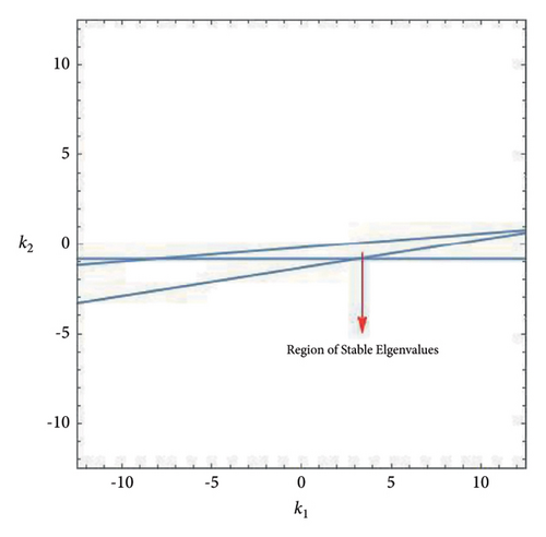
Then, stable eigenvalues lie within the triangular region (k1k2)-plane bounded by the straight lines L1,2,3 for parametric values a, b, c, d, e, and τ.

Remark 15. In the context of a discrete prey-predator model, feedback gains k1 and k2 play a crucial role in controlling the system’s dynamics using the OGY method. These feedback gains are typically parameters that determine the strength and nature of the feedback loop regulating the interactions between the predator and prey populations. More specially, k1 represents the influence of the predator population on the prey population dynamics. A higher value of k1 implies stronger regulation of the prey population growth by predation. In biological terms, this could correspond to factors such as predation pressure or the efficiency of predators in hunting prey. For instance, if k1 is high, it suggests that predators have a significant impact on controlling prey population growth, reflecting a scenario where predation is a dominant factor in shaping prey dynamics. On the other hand, k2 reflects the influence of the prey population on the predator population dynamics. A higher value of k2 implies stronger regulation of predator population growth by prey availability. In biological terms, this could represent factors such as prey abundance or the efficiency of predators in capturing prey. If k2 is high, it suggests that prey availability strongly influences predator population dynamics, indicating a scenario where prey abundance is a key determinant of predator population size.

5.2. By Hybrid Control Feedback

We use a hybrid control feedback to control the chaos due to the emergence of flip bifurcation in model (7) by the existing theory [37]. If model (7) undergoes bifurcation at φ3, then one can write corresponding controlled model as
(105)
where 0 < α < 1 and controlled strategy (105) is a combination of feedback control as well as parameter perturbation. The is
(106)
The characteristics equation of is
(107)
where
(108)

So, based on the stability theory, one has the result.

Lemma 16. Equilibrium φ3 of model (105) is a sink iff |2 + α(a − 1 − (2ac/bτ) − (2beτ(bτ(a − 1) − ac)/c2 + b2eτ2))| < 2 + α(a − 1 − (2ac/bτ) − (2beτ(bτ(a − 1) − ac)/c2 + b2eτ2)) + (α2c(bτ(a − 1) − ac)/bτ) < 2.

Remark 17. In the context of real ecosystems and considering current ecological knowledge, chaos control emerges as a crucial concept when addressing disruptions such as Neimark–Sacker and flip bifurcations. These disruptions, reflecting our awareness of the complex and nonlinear nature of ecological systems, can introduce chaotic dynamics, same as unpredictable fluctuations in predator and prey interactions. Chaos control strategies, informed by contemporary ecological insights, play a pivotal role in mitigating the impact of these disruptions. By understanding the factors that lead to chaotic behavior, ecologists can implement control measures to guide the system back to a stable and predictable state. This might involve adjusting key ecological parameters, introducing adaptive management practices, or leveraging technological advancements to intervene in the ecosystem’s dynamics. In the application of chaos control within real ecosystems, the goal is not only to prevent ecological chaos but also to enhance the overall resilience and sustainability of the system. Harnessing current ecological knowledge, scientists strive to develop and implement effective chaos control strategies that contribute to the preservation of biodiversity, the stability of populations, and the health of ecosystems. In this way, chaos control becomes an integral component of ecological management, aligning with our evolving understanding of the intricate relationships within natural systems. In short, when real ecosystems face disruptions such as N-S and flip bifurcations, scientists use chaos control strategies, guided by what we know about nature. It is like fixing a dance that has gone a bit wild. By understanding and managing these disruptions, we aim to bring stability back to the way animals interact in nature. This helps keep the environment healthy and ensures that both nature and the communities relying on it can thrive together. Our growing knowledge of ecology acts as a guide, leading us to more effective ways of maintaining a balanced and sustainable relationship between different species.

6. Numerical Simulations

In this section, we will present some simulation for the correctness of theoretical results. All plots have been drawn by Mathematica and MATLAB software.

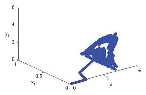
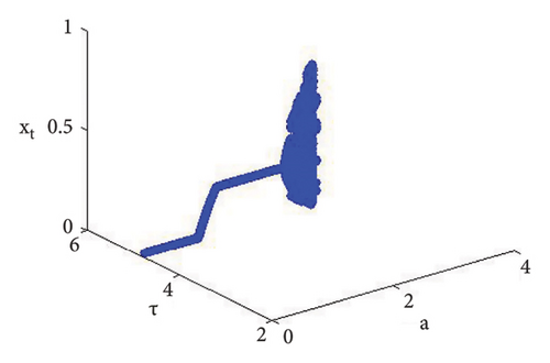
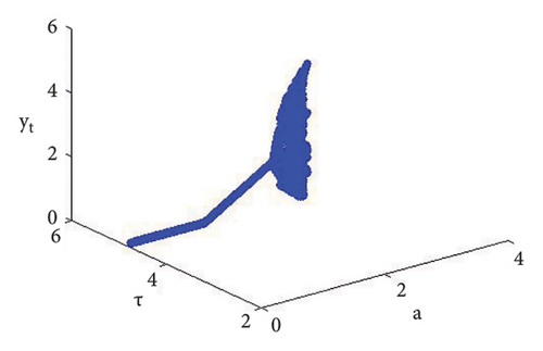
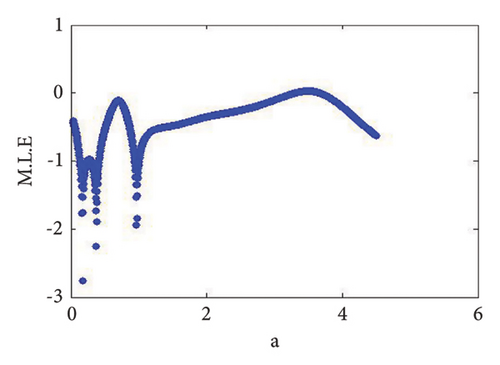
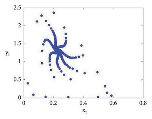
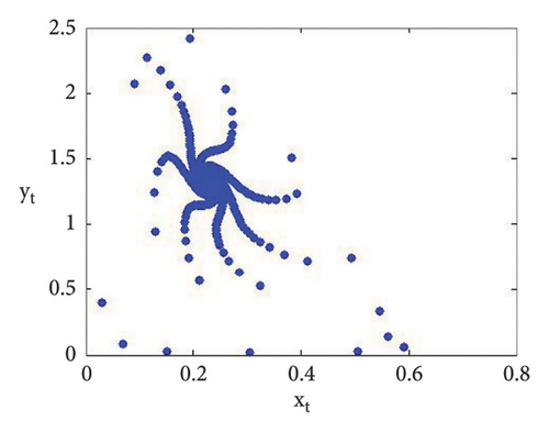
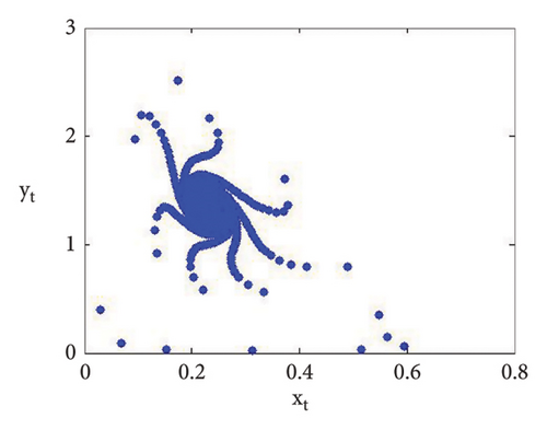
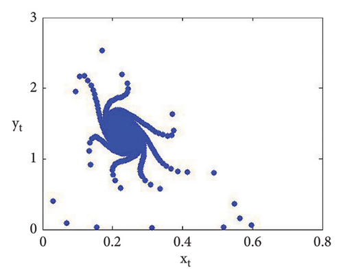
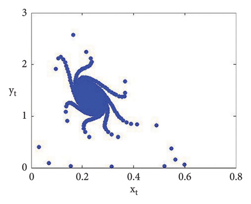
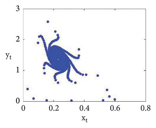
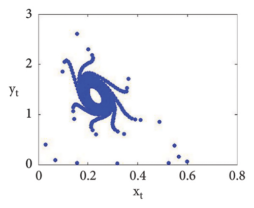
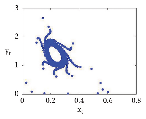
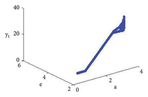
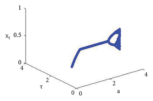
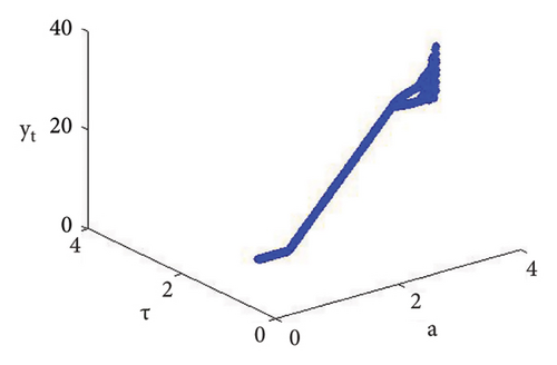
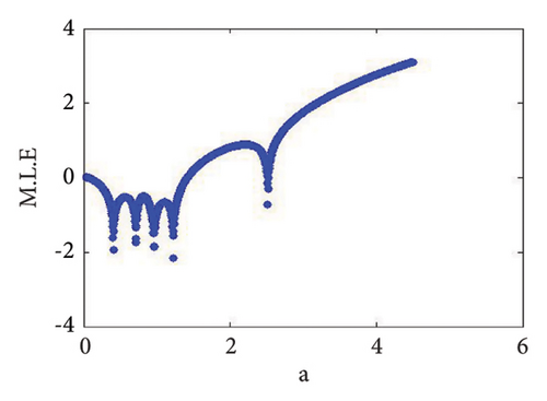
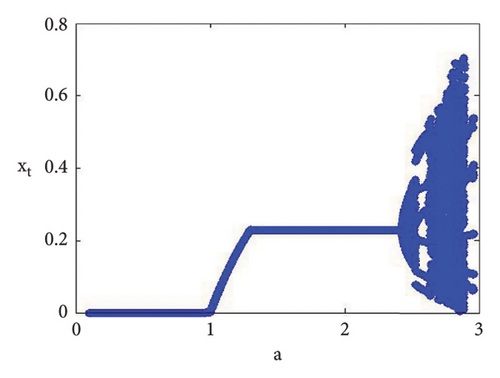
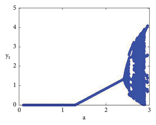
Example 1. If d = 0.4, c = 0.9, b = 0.8, e = 0.09, τ = 4.9, and a = [0.1, 2.99] with (x0, y0) = (0.03, 0.4), then N-S bifurcation exist for model (7) at a = 2.433366930993503. The Maximum Lyapunov exponent with bifurcation diagrams are drawn in Figure 1. In addition, at (c, b, d, e, τ, a) = (0.8, 0.9, 0.4, 0.09, 4.9, 2.433366930993503), model (7) has interior equilibrium point φ3 = (0.22959183673469383, 1.3592438014406019) and moreover, from (19), one gets

(109)
with
(110)

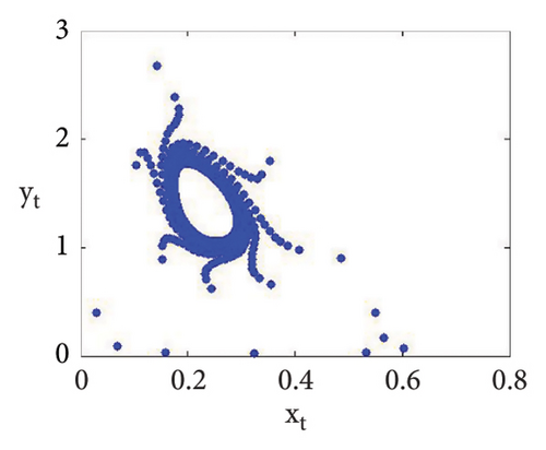
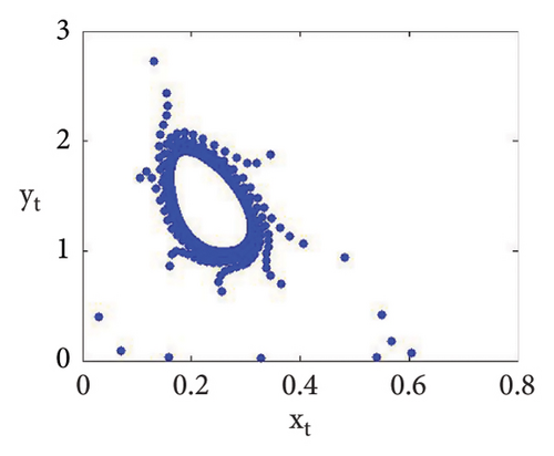
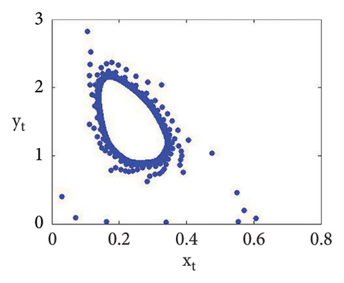
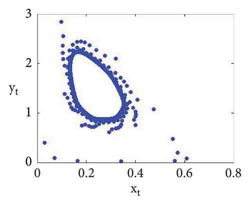
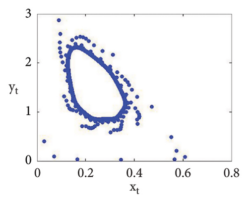
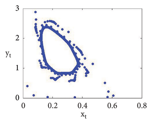
The roots of (110) are λ1,2 = 0.6063914134642423 ± 0.7951663056724918ι with |λ1,2| = 1, and so from (i) of Theorem 10, one gets . Furthermore, if we fixed c = 0.9, b = 0.8, d = 0.4, e = 0.09, and τ = 4.9 and varying a < 2.433366930993503, that is, a = 2.38877, a = 2.39999, 2.40099, 2.41999, 2.42444, 2.43119 < 2.433366930993503, then Figures 2(a), 2(b), 2(c), 2(d), 2(e), and 2(f) clearly indicate that respective equilibria is stable focus. On contrary, we get the unstable focus if a > 2.433366930993503, and in addition, as a result, supercritical N-S bifurcation takes place. For example, if b = 0.8, c = 0.9, d = 0.4, e = 0.09, and τ = 4.9, then from (32), one gets holds, and moreover, if a = 2.433366930993503, then from (134) and (135), one gets

(111)
and
(112)

Utilizing (111) and (112) into (135), one gets

(113)

Now in view of (41) and (113), one obtains

(114)

Now, using (114) with into (39), we get . This indicates that closed invariant curve appears, and at φ3 = (0.22959183673469383, 1.3592438014406019), supercritical N-S bifurcation exists (see Figure 3(a)). Same behavior exists for the discrete model (7) at respective fixed points if a = 2.43999, 2.44999, 2.45641, 2.46999, 2.49999, 2.50999, 2.52111, and 2.53000 > 2.433366930993503 (see Figures 3(a), 3(b), 3(c), 3(d), 3(e), 3(f), 3(g), 3(h), and 3(i)). Therefore, in conclusion, we can say that numerical simulations in Example 1 agree with theoretical results obtained in Theorem 8(i) of Theorems 10 and 12.
Details are in the caption following the image
MLE and bifurcation diagrams for (a) xt. (b) yt. (c) xt and yt. (d) τ and xt. (e) τ and yt. (f) MLEs.
Details are in the caption following the image
MLE and bifurcation diagrams for (a) xt. (b) yt. (c) xt and yt. (d) τ and xt. (e) τ and yt. (f) MLEs.
Details are in the caption following the image
MLE and bifurcation diagrams for (a) xt. (b) yt. (c) xt and yt. (d) τ and xt. (e) τ and yt. (f) MLEs.
Details are in the caption following the image
MLE and bifurcation diagrams for (a) xt. (b) yt. (c) xt and yt. (d) τ and xt. (e) τ and yt. (f) MLEs.
Details are in the caption following the image
MLE and bifurcation diagrams for (a) xt. (b) yt. (c) xt and yt. (d) τ and xt. (e) τ and yt. (f) MLEs.
Details are in the caption following the image
MLE and bifurcation diagrams for (a) xt. (b) yt. (c) xt and yt. (d) τ and xt. (e) τ and yt. (f) MLEs.
Details are in the caption following the image
Phase portrait with (0.03, 0.4) if (a) a = 2.38877. (b) a = 2.39999. (c) a = 2.40099. (d) a = 2.41999. (e) a = 2.42444. (f) a = 2.43119.
Details are in the caption following the image
Phase portrait with (0.03, 0.4) if (a) a = 2.38877. (b) a = 2.39999. (c) a = 2.40099. (d) a = 2.41999. (e) a = 2.42444. (f) a = 2.43119.
Details are in the caption following the image
Phase portrait with (0.03, 0.4) if (a) a = 2.38877. (b) a = 2.39999. (c) a = 2.40099. (d) a = 2.41999. (e) a = 2.42444. (f) a = 2.43119.
Details are in the caption following the image
Phase portrait with (0.03, 0.4) if (a) a = 2.38877. (b) a = 2.39999. (c) a = 2.40099. (d) a = 2.41999. (e) a = 2.42444. (f) a = 2.43119.
Details are in the caption following the image
Phase portrait with (0.03, 0.4) if (a) a = 2.38877. (b) a = 2.39999. (c) a = 2.40099. (d) a = 2.41999. (e) a = 2.42444. (f) a = 2.43119.
Details are in the caption following the image
Phase portrait with (0.03, 0.4) if (a) a = 2.38877. (b) a = 2.39999. (c) a = 2.40099. (d) a = 2.41999. (e) a = 2.42444. (f) a = 2.43119.
Details are in the caption following the image
Invariant closed curves with (0.03, 0.4) if (a) a = 2.43444. (b) a = 2.43999. (c) a = 2.44999. (d) a = 2.45641. (e) a = 2.46999. (f) a = 2.49999. (g) a = 2.50999. (h) a = 2.52111. (i) a = 2.53000.
Details are in the caption following the image
Invariant closed curves with (0.03, 0.4) if (a) a = 2.43444. (b) a = 2.43999. (c) a = 2.44999. (d) a = 2.45641. (e) a = 2.46999. (f) a = 2.49999. (g) a = 2.50999. (h) a = 2.52111. (i) a = 2.53000.
Details are in the caption following the image
Invariant closed curves with (0.03, 0.4) if (a) a = 2.43444. (b) a = 2.43999. (c) a = 2.44999. (d) a = 2.45641. (e) a = 2.46999. (f) a = 2.49999. (g) a = 2.50999. (h) a = 2.52111. (i) a = 2.53000.
Details are in the caption following the image
Invariant closed curves with (0.03, 0.4) if (a) a = 2.43444. (b) a = 2.43999. (c) a = 2.44999. (d) a = 2.45641. (e) a = 2.46999. (f) a = 2.49999. (g) a = 2.50999. (h) a = 2.52111. (i) a = 2.53000.
Details are in the caption following the image
Invariant closed curves with (0.03, 0.4) if (a) a = 2.43444. (b) a = 2.43999. (c) a = 2.44999. (d) a = 2.45641. (e) a = 2.46999. (f) a = 2.49999. (g) a = 2.50999. (h) a = 2.52111. (i) a = 2.53000.
Details are in the caption following the image
Invariant closed curves with (0.03, 0.4) if (a) a = 2.43444. (b) a = 2.43999. (c) a = 2.44999. (d) a = 2.45641. (e) a = 2.46999. (f) a = 2.49999. (g) a = 2.50999. (h) a = 2.52111. (i) a = 2.53000.
Details are in the caption following the image
Invariant closed curves with (0.03, 0.4) if (a) a = 2.43444. (b) a = 2.43999. (c) a = 2.44999. (d) a = 2.45641. (e) a = 2.46999. (f) a = 2.49999. (g) a = 2.50999. (h) a = 2.52111. (i) a = 2.53000.
Details are in the caption following the image
Invariant closed curves with (0.03, 0.4) if (a) a = 2.43444. (b) a = 2.43999. (c) a = 2.44999. (d) a = 2.45641. (e) a = 2.46999. (f) a = 2.49999. (g) a = 2.50999. (h) a = 2.52111. (i) a = 2.53000.
Details are in the caption following the image
Invariant closed curves with (0.03, 0.4) if (a) a = 2.43444. (b) a = 2.43999. (c) a = 2.44999. (d) a = 2.45641. (e) a = 2.46999. (f) a = 2.49999. (g) a = 2.50999. (h) a = 2.52111. (i) a = 2.53000.

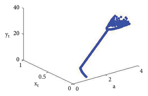
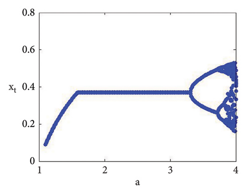
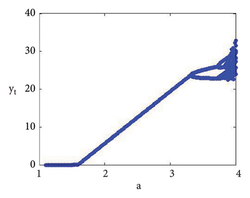
Example 2. If b = 0.6, c = 0.4 = d, e = 3.1, τ = 1.8, and a = [1.1, 4.0] with (x0, y0) = (0.2, 0.3), then flip bifurcation exists at a = 3.3084030868763388 where MLE with flip bifurcation diagrams are presented in Figure 4. Furthermore, at (b, c, d, e, τ, a) = (0.6, 0.4, 0.4, 3.1, 1.8, 3.3084030868763388), one has φ3 = (0.37037037037037035, 23.666051975387873) and moreover, from (19), one gets

(115)
with λ1 = −1 and λ2 = 0.7833862779489057 ≠ 1 or  − 1. So, . Moreover, in this parametric domain, from (47), (49), (50), and (136), one gets
(116)
(117)
and
(118)

Utilizing (118) into (51), one gets and . Since , and so stable period-2 points bifurcate from φ3 = (0.37037037037037035, 23.666051975387873). Therefore, in conclusion, we can say that numerical simulations in Example 2 agree with theoretical results obtained in Theorem 9(ii) of Theorems 10 and 13.
Details are in the caption following the image
MLE and flip B.Ds for (a) xt. (b) yt. (c) xt and yt. (d) e and xt. (e) e and yt. (f) τ and xt. (g) τ and yt. (h) MLEs.
Details are in the caption following the image
MLE and flip B.Ds for (a) xt. (b) yt. (c) xt and yt. (d) e and xt. (e) e and yt. (f) τ and xt. (g) τ and yt. (h) MLEs.
Details are in the caption following the image
MLE and flip B.Ds for (a) xt. (b) yt. (c) xt and yt. (d) e and xt. (e) e and yt. (f) τ and xt. (g) τ and yt. (h) MLEs.
Details are in the caption following the image
MLE and flip B.Ds for (a) xt. (b) yt. (c) xt and yt. (d) e and xt. (e) e and yt. (f) τ and xt. (g) τ and yt. (h) MLEs.
Details are in the caption following the image
MLE and flip B.Ds for (a) xt. (b) yt. (c) xt and yt. (d) e and xt. (e) e and yt. (f) τ and xt. (g) τ and yt. (h) MLEs.
Details are in the caption following the image
MLE and flip B.Ds for (a) xt. (b) yt. (c) xt and yt. (d) e and xt. (e) e and yt. (f) τ and xt. (g) τ and yt. (h) MLEs.
Details are in the caption following the image
MLE and flip B.Ds for (a) xt. (b) yt. (c) xt and yt. (d) e and xt. (e) e and yt. (f) τ and xt. (g) τ and yt. (h) MLEs.
Details are in the caption following the image
MLE and flip B.Ds for (a) xt. (b) yt. (c) xt and yt. (d) e and xt. (e) e and yt. (f) τ and xt. (g) τ and yt. (h) MLEs.

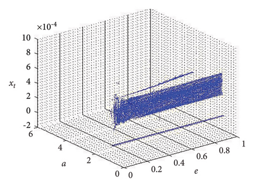
Example 3. If d = 1.9, b = 2.5, τ = 10.98, and c = 0.99, then from (56) the calculation yields e = 0.04460034922732295 and a = 5.228990586133444. Therefore, if (d, b, τ, c, e, a) = (1.9, 2.5, 10.98, 0.99, 0.04460034922732295, 5.228990586133444), then model (7) has φ3 = (0.0360655737704918, 2.706457459921495) and moreover, from (20), one gets

(119)
with λ1,2 = −1 and so . Now, from (71) and (86), one conclude the following results:
(120)

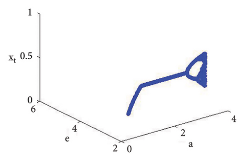
Using (120) into (85), one gets C = −223.52473751174273 ≠ 0 and D = 24628.549545279584 ≠ 0, D + 3 = 2.46 × 10⁴ ≠ 0. This indicates that codimension-two bifurcation with 1 : 2 strong resonance bifurcation exists, which is depicted in Figure 5.
Details are in the caption following the image
Codimension-two bifurcation diagram at φ3.
Details are in the caption following the image
Codimension-two bifurcation diagram at φ3.

Example 4. Here, bifurcation parameter a is chosen as a controlled parameter, and so reconsider the data (d, b, c, e, τ, a) = (0.4, 0.8, 0.9, 0.09, 4.9, 2.433366930993503) as in Example 1; the MLE with bifurcation diagrams are same as in Figure 1. In order to apply the OGY control method for model (7), if a0 = 3.99, then it has equilibrium φ2 = (0.22959183673469383, 3.2228426749271137). So, model (97) becomes

(121)
where its variation matrix VBK is
(122)

Now, for marginal stability lines L1, L2, and L3 are

(123)
(124)
and
(125)

So, lines (123)–(125) experience the region where |λ1,2| < 1 (see Figure 6).
Details are in the caption following the image
Region of stability where |λ1,2| < 1.

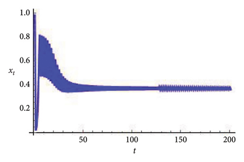
Example 5. Finally, if b = 0.6, c = 0.4 = d, e = 3.1, τ = 1.8, a = 3.3084030868763388 with (x0, y0) = (0.98, 0.5), then model (7) undergoes flip bifurcation. For this, by applying the hybrid strategy to get stable orbit at φ3 = (0.37037037037037035, 23.666051975387873). For this model, (105) takes the form

(126)
where is
(127)
(128)

Furthermore, roots of (128) satisfy |λ1,2| < 1 if 0 < α < 1. So, for the allowed interval of control parameter α the flip bifurcation is completely eliminated. If α = 0.999, then for controlled model (126), plots of t vs. xt and yt are drawn in Figure 7.
Details are in the caption following the image
Plot of t vs. xt and yt for controlled system (91).
Details are in the caption following the image
Plot of t vs. xt and yt for controlled system (91).

Remark 18. The convergence speed of a prey-predator model, depicting the dynamic interactions between predator and prey populations, is subject to various parameters (influential factors). Foremost among these factors are the interaction parameters that govern the dynamics of predation, reproduction, and efficiency in capturing prey. Fine-tuning these parameters can significantly impact the speed at which the model converges to a stable solution. In addition, the initial conditions set for the simulation play a critical role and carefully chosen distributions and densities of prey and predators can contribute to faster convergence, reflecting realistic ecological scenarios. Maintaining a delicate balance between prey and predator populations is crucial for efficient convergence. Extreme imbalances may impede the model’s ability to reach a stable equilibrium, affecting the overall convergence speed. Environmental factors, such as resource availability and habitat quality, further influence the dynamics and, consequently, the speed at which the model converges. The complexity of the mathematical model itself, including its level of sophistication or simplicity, can also impact convergence speed. Considerations such as the choice of numerical methods, the size of time steps, and the presence of adaptation mechanisms add additional layers of complexity that can either expedite or hinder the convergence process. In summary, a comprehensive understanding and strategic adjustment of these factors are essential for optimizing the convergence speed of a prey-predator model, ensuring a more accurate and insightful representation of ecological dynamics. Our results underscore the intricate interplay of factors affecting the convergence speed in the prey-predator model. The observed sensitivity to parameter values and initial conditions emphasizes the need for a nuanced approach in calibrating the model for accurate and efficient simulations. Through this iterative process of parameter exploration and adjustment, a deeper understanding of the dynamics and equilibrium states in the simulated ecosystem has been achieved.

Remark 19. The connection between the bifurcation diagram and the MLE diagram is important to understanding the dynamic behavior of nonlinear systems. The bifurcation diagram represents transitions between stable and chaotic states by graphically representing the qualitative changes in a system as a parameter is varied. In addition, the MLE serves as a quantitative measure of the system’s sensitivity to initial conditions, particularly in chaotic regimes. Bifurcation region associated with transitions to chaos often align with peaks in the MLE diagram, indicating high rates of divergence in trajectories. Together, these diagrams provide complementary insights into the stability and predictability of a dynamic system. The bifurcation diagram offers a visual representation of the system’s behavior, while the MLE quantifies the degree of chaos, allowing for a more comprehensive understanding of the intricate dynamics governing nonlinear systems. MLE can help to resolve some of these ambiguities by quantifying the degree of chaos in a system. MLE is defined as the average exponential rate of divergence (or convergence) of two nearby trajectories in the phase space of a system. A positive MLE indicates that the system is chaotic, since small perturbations will grow exponentially over time. A negative MLE indicates that the system is stable since nearby trajectories will converge to a fixed point or a periodic orbit. A zero MLE indicates that the system is marginally stable since nearby trajectories neither diverges nor converges.

7. Preservation of the Positivity

In this section, we study preservation of the positive solution of the discrete model (7) based on the existing work [38]. Suppose that xt,  yt ≥ 0 for some tN, the parameters b and τ are positive, then the second equation of the discrete prey-predator model (7) implies that 1 + bτxtc ≥ 0 for c ∈ (0, 1). Furthermore, from first equation of model (7), xt+1 ≥ 0 necessitates . So, the condition that ensure the positivity of the solution of the discrete prey-predator model (7) is (xt, yt) ∈ Δ where
(129)
In addition, from model (7), one define by
(130)
Now, assume that (x0, y0) ∈ Δ, then xt, yt ≥ 0 for each tN if F(Δ) = Δ where
(131)
with
(132)
and
(133)

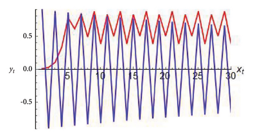
On performing straightforward computation by Mathematica, one obtain that F1(Δ) = Δ, if α ∈ (0, 4), b < 1, c ∈ (0, 1) and τ ≤ 6.8 where Figure 8(a) shows the positive nature of model (7). On contrary, Figure 8(b) shows the negative behavior of the discrete prey-predator model (7) if α > 4, b = 1, c = 1.1 and τ = 6.9.

Details are in the caption following the image
(a) Positive behavior of the discrete prey-predator model (7) if α ∈ (0, 4), b < 1, c ∈ (0, 1) and τ ≤ 6.8 with (x0, y0) = (0.009, 0.9). (b) Negative behavior of the model (7) if α > 4, b = 1, c = 1.1 and τ = 6.9.
Details are in the caption following the image
(a) Positive behavior of the discrete prey-predator model (7) if α ∈ (0, 4), b < 1, c ∈ (0, 1) and τ ≤ 6.8 with (x0, y0) = (0.009, 0.9). (b) Negative behavior of the model (7) if α > 4, b = 1, c = 1.1 and τ = 6.9.

8. Conclusion

The work is about local dynamics, chaos, and codimension-one and codimension-two bifurcations of a discrete prey-predator model (7). It is proven that model (7) has trivial, semitrivial, and interior fixed points algebraically. We have studied local dynamics at fixed points by the linear stability theory. In order to study the bifurcation analysis at equilibria, we first identified codimension-one bifurcation sets for the understudied model and then it proved that at the semitrivial fixed point, the model (7) undergoes flip bifurcation. Furthermore, at the interior fixed point, we have examined that model (7) undergoes Neimark–Sacker and flip bifurcations if parameter goes through the certain curves, and at this point, we also studied codimension-two 1 : 2 strong resonance bifurcation analysis. Next, OGY and hybrid control strategies are employed to manage chaos in the model under study, which arises from Neimark–Sacker and flip bifurcations, respectively. We have examined the preservation of the positive solution of the discrete prey-predator model (7). Finally, numerical simulations are given to verify the theoretical results. Our numerical simulations reveal that at the interior fixed point, model (7) undergoes supercritical Neimark–Sacker, which implies that there exist quasiperiodic or periodic oscillations between prey and predator individuals.

In our exploration, we delved into the dynamics of a prey-predator model by employing linear stability theory, a well-established method in existing literature for studying bifurcations. The model (7)’s interior fixed point became a focal point of our investigation, revealing significant insights into its behavior, particularly through the identification of Neimark–Sacker (N-S) and flip bifurcations. The recognition of these bifurcations enhances our understanding of how the prey and predator populations undergo qualitative changes, introducing a layer of complexity to their interactions. In addition, we extended our study to chaos control within the prey-predator model. Chaos control strategies were implemented to navigate and regulate the system’s behavior, providing a means to influence and stabilize the dynamics, especially in the context of the recognized N-S and flip bifurcations. The application of chaos control techniques adds a practical dimension to our research, offering potential tools for managing and steering the prey-predator system towards more predictable and stable states. By combining insights from the linear stability theory, bifurcation analysis, and chaos control strategies, our study contributes to the comprehensive understanding of the prey-predator model’s behavior. This knowledge not only enriches the existing literature on ecological dynamics but also provides practical implications for ecosystem management and conservation efforts, showcasing the interdisciplinary nature of our research approach.

8.1. Future Direction

The study of codimension-two 1 : 3 and 1 : 4 strong resonance bifurcation analysis and global dynamics of the discrete model (7) is our next aim to study.

8.1.1. Expression for the Coefficients Quantities of System (35)

(134)

8.1.2. Expression for the Coefficients Quantities of System (38)

(135)

8.1.3. Expression for the Coefficients Quantities of System (42)

(136)

Conflicts of Interest

The authors declare that they have no conflicts of interest.

Acknowledgments

This study was supported via funding from Prince Sattam bin Abdulaziz University (project number PSAU/2024/R/1445).

    Data Availability

    No data were used to support the findings of this study.

      The full text of this article hosted at iucr.org is unavailable due to technical difficulties.