Malaria is an old, curable vector-borne disease that is devastating in the tropics and subtropical regions of the world. The disease has unmatched complications in the human host, especially in children. Mathematical models of infectious diseases have been the steering wheel, driving scientists towards elucidation of the dynamic behaviour of epidemics and providing tailored strategic management of diseases. With the ongoing vaccination programs for vector-borne diseases, the research proposes a nonlinear differential equation model for the malaria disease that provides public health with a shift from the classical understanding of nonpharmaceutical preventive malaria control to pharmaceutical measures of vaccines. The asymptotic dynamic behaviour of the model is studied at the model’s equilibria. The bifurcation type invoked at the disease-free state is analysed, and the result revealed that the convention that is the condition for eradicating the disease is not always sufficient when the system undergoes backward bifurcation. Furthermore, sensitivity analysis was investigated to quantify the amount of influence each parameter has on . With the Latin hypercube sampling and partial rank correlation coefficient method, the uncertainty in is computed with a 95% confidence interval, with the mean, and 5th and 95th percentiles, respectively, simulated as 0.143788, 0.01545, and 0.41491. An intervention model was derived from the nonintervention model to experiment with and evaluate the respective effects of the various pairings of interventions on the dynamics of the disease. Lastly, an in-depth cost analysis was studied to identify the most cost-effective intervention regarding rewarding the desired outcome. From the analysis, we recommend that besides the nonpharmaceutical measure of bed nets and insecticide spray, public health should target the pharmaceutical intervention of vaccine as it can close the gap in malaria prevention.

1. Introduction

Malaria is one of the most curable vector-borne diseases in the world, predominating in tropical and subtropical regions where the weather and change in climate favour the disease transmission [1]. Even though many eradication programs have been carried out, the disease remains endemic in these climate-favoured regions. The disease, over the years, has been a sting on the human race, causing both economic and social burdens through illness and death, and is recognised as one of the longest-known vector-borne health concerned diseases. In the 2022 report of the World Health Organization [2], an estimated 249 million and 608,000 malaria cases and deaths were reported. The estimates mean that in 2022, a hike of 5 million in additional cases was reported. In the WHO African region, 233 million cases of global Malaria cases were reported. The report constitutes 94% of malaria cases. The burden of the disease in Africa is alarming that billions of dollars are spent yearly by governments for prevention and treatment services [3]. The disease is noted for its sensitivity to changing climatic conditions, with hot temperatures favouring the growth of the vector and multiplying transmissibility [4]. Recently, death related to malaria incidence has lowered significantly. However, cases of malaria incidence are on a surge in some metropolitans and local communities. The current epidemic surge in both metropolitans and local communities substantially reflects the changing dynamics of malaria transmission, with communities identified as free malaria regions witnessing higher cases and places marked as endemic areas having fewer cases. Areas of disease dominance include Africa, Asia, the Americas, and the Caribbean, with the disease endemic in regions with escalating sanitation problems. After a hurdle of many struggles, a significant landmark has been reached in vaccine development. In October 2021, the World Health Organization regulatory body endorsed the first-ever malaria vaccine, a breakthrough for vector-borne diseases [5]. Expectedly, the vaccine roll-out with other known malaria control measures such as sleeping under an insecticide-treated net and indoor and outdoor residual spray has pushed down the number of infected and hospitalized [6].

Mathematical modelling has been the framework for providing dynamic insight into disease transmission and phenomenon to stakeholders and intervention strategies needed to put in place for the optimum solution ([7–13]). The study of Tumwiine, Mugisha, and Luboobi [14] proposed a nonlinear model for malaria disease that captured human recruitment via repeated immigration. The study determined the model’s equilibria and carried out a global asymptotic stability analysis of the model’s equilibria. Sabbar, Yavuz, and Özköse [15] considered a general epidemic model that analysed the effect of stochasticity on the dynamic behaviour of extinction disease. Penny et al. [16] examined the cost-effective analysis of the malaria vaccine and its impact on the transmission of the disease by considering four models of malaria. Studies of Romero-Leiton and Ibargüen-Mondragón [17] considered a mathematical model of malaria disease that is segregated into eight compartments that determined to elucidate the dynamic behaviour of the epidemic in Tumaco, Colombia. The study examined the local and global dynamic stability behaviour at the model’s steady states. Further, the condition that leads to backward or forward bifurcation is determined. The model is then modified to optimal control by capturing time-dependent controls. Lastly, economic cost analysis is studied of the proposed strategies to find the optimum strategy. Research conducted by B. Traoré, Sangaré, and S. Traoré [18] proposed a nonlinear malaria model that factored the different developmental stages of the vector into consideration. The study, in addition, examined the impact of change in climate on the metamorphic life cycle of the vector. The global qualitative analysis of the model was studied to explore the dynamic behaviour of the epidemic’s steady states. The analysis showed that the global behaviour is dependent on the humans’ and the vector’s effective reproduction number, . In [19], the authors constructed a malaria model that explored the dynamic behaviour at the endemic state. The was derived analytically, and the existence of the malaria-free point when is less than one was proved. A perturbation analysis of the model was explored to approximate the endemic point. Stochastic perturbation is then applied to the model, resulting in a stochastic system. A numerical solution is provided for the models. The analyses showed that due to the stochastic variability, the infected people in the population are not constant but undergo fluctuations. In the study of Oke et al. [20], a deterministic malaria model was proposed that used differential equation tools to analyse the stability at the equilibria. The model determined controls for the dynamical system such that the objective function is optimized over a time frame. The impact of the identified controls on the infected individuals was investigated. The investigation results indicated that the pairing of the controls—treated bednet, medication, and insecticide spraying—substantially impacts the infectives by significantly minimizing it. In [21], the authors modelled a transmission model of malaria disease that primarily assessed the linearity of the ’s parameters and their impact on the . Further, measures that target the biting rate of the vector were identified. The model result proved that interventions that targeted the biting rate of the vector successfully controlled the epidemic. In the work of Huo and Qiu [22], a transmission model of malaria disease which considered the returning of infected humans not only to the susceptible compartment but to the infective as well is proposed. The model’s stability analysis at the steady states was carried out, which showed the persistence of the infection when R₀ > 1 and the global asymptotic dynamic behaviour of the disease when R₀ ≤ 1. Orwa, Mbogo, and Luboobi [23] considered a nonlinear compartmental malaria model that captured the liver stage to the blood stage of the parasite development and examined the impact of immune response and treatment on the disease transmission. The qualitative model analysis was studied, which revealed the asymptotic stability of the disease-free state locally and globally. In Ducrot et al.’s study [24], a malaria model that captured the two natures of the human host—semi-immune and nonimmune—was proposed. The condition that leads to backward or forward bifurcation is examined. Finally, measures to curb the disease were explored for the associated subgroup of semi-immune, nonimmune, and vector. From the studies of Yang [25], a compartmental model of malaria transmission is constructed that examines the impact of global warming on the dynamics of the disease. The model carried out an explicit derivation of the R₀. The analytic method of sensitivity analysis was applied to the model to assess the different scenarios when the model’s parameters are varied. The article by Nana-Kyere et al. [26] proposed an optimal intervention model with time-dependent controls that were qualitatively and numerically solved to find the optimum eradication measure for the disease. Arquam, Singh, and Cherifi [27] proposed and examined a data-inspired SIR vector-borne model that assessed the temperature variations’ effect on vector-borne diseases. The study of Iggidr, Sallet, and Souza [28] examined the dynamics of multigroup vector-borne diseases, an extension of the Bailey–Dietz model. The research of Kuniyoshi and Santos [29] employed the variant SIR model type to analyse the effect of insecticide resistance on vector-borne diseases. The authors in [30] considered a SIR model for a vector-transmitted disease incorporating an age-structured vaccinated population to examine the impact of vaccines on the disease dynamics. They applied the results from the analysis to study dengue fever disease. Using the classical SIR model, the authors in [31] assessed the impact of mathematical models on intervention provision directed at managing vector-borne diseases. In the study of [32], a compartmentalized SEIR-SEI vector-borne model of host–vector is utilised to predict dengue outbreak. The model also estimated the epidemic’s important parameters by fitting it to actual dengue fever data. Smith et al. [33] developed a mathematical model for the malaria epidemic that assessed vaccines’ impact on the disease dynamics by fitting the model to field malariology datasets from several portions of Africa. In a related study of [34], a climate model that assessed the rainfall and temperature variability influence on the vector–host malaria model is considered. The model was fitted to malaria transmission data of Limpopo Province, South Africa, to determine all the malaria spikes in the province. The study of White et al. [35] employed the clinical trial data to estimate the efficacy of the RTS malaria vaccine profile using mathematical models. The study further illustrated how clinical trial estimated parameters can be utilised to forecast vaccination campaign impacts on the disease. Slater, Okell, and Ghani [36] explored the effects of integrating two factors: pharmacokinetic and pharmacodynamic in drug design on the malaria transmission dynamics in humans using mathematical models. The study demonstrated that the two therapies are the key to eliminating the disease. In Olaniyi et al.’s study [37], a malaria model that accounted for the different transmission trends in a social hierarchy-structured population was proposed. A new optimal control model was developed to examine the proposed strategies’ efficiency. The cost-effectiveness analysis was considered to determine the most cost-effective strategy of the considered strategies. In [38], a mathematical model describing vector–host transmissibility dynamics is considered that focused primarily on the maturity delay of the vector. In [39], a malaria transmissibility model was proposed that examined the effect of the vaccine on the model’s dynamics. The analyses showed that a vaccine would minimize secondary infections when it minimizes the infectious period of the disease. Using the curve fitting technique, Nana-Kyere, Seidu, and Nantomah [40] calibrated a mathematical model in the context of Ghana that investigated the substantial intervention program for containing the disease in Ghana.

With the ongoing vaccination program for vector-borne diseases, the research primarily focuses on deriving a mathematical model for the malaria epidemic that would provide public health with a shift from the classical understanding of nonpharmaceutical preventive malaria control to the pharmaceutical measure of vaccines by quantifying the potency of vaccines in eradicating the disease. The research would provide the public health decision body, a valuable insight into the significant contribution of vaccines, by reducing the overall disease burden and incidence, hospitalization, and death resulting from malaria disease.

The design of the research is as follows: The derivation of the Malaria model and demonstration of the model’s positivity and boundedness are presented in Section 2. Section 3 is devoted to the computation of , assessment of the local stability of model system (1) at the model’s equilibria, and exploring the global stability of model system (1) at model’s equilibria, bifurcation study, global sensitivity analysis, and vaccine efficacy assessment. Section 4 redesigns the model system (1) to the intervention model to explore interventions that would help mitigate the disease. The section furthermore provided numerical simulations for the models to complement the analytic analyses. In Section 5, cost-effective analysis is studied to let stakeholders know which interventions to prioritize in their attempt to curb the menace. Section 6 provides a thorough discussion and conclusion based on the outcome of the investigation.

2. Derivation of the Malaria Model

The present section formulates a nonlinear differential equation model for malaria disease that segregates the population into susceptible humans, S_H; exposed humans, E_H; vaccinated humans, V_H; asymptomatic humans, A_H; mildly infected humans, I_H1; severely infected humans, I_H2; and recovered humans, R_H. The model assumes that the mildly infected are individuals who are showing symptoms of the disease but are not in the acute stage, while the severely infected individuals are those in the acute stage of the disease. Hence, the human population N_H is denoted as follows: N_H = S_H + V_H + E_H + A_H + I_H1 + I_H2 + R_H. The vector has a population given by N_V = S_V + E_V + I_V, with S_V, denoting susceptible mosquitoes, E_V, the exposed mosquitoes, and I_V, the infected mosquitoes. The model assumes that recruitments of susceptible humans and susceptible mosquitoes into the human and vector populations are, respectively, given by Λ_a and Λ_b. β₁ and β₂ represent the pathways of transmission from mosquitoes to humans and humans to mosquitoes. α denotes the biting rate of mosquitoes. The transition from the exposed to the asymptomatic human is given by the rate ψ_a. ϕ_a also denotes the transition from asymptomatic to mildly infected humans. σ_a is the rate at which the mildly infected humans progress to severely infected human status. γ_a represents the recovery rate of the severely infected humans. Further, σ₁ represents the death of severely infected humans owing to the disease. δ₁, δ₂ are the recovery rates of the asymptomatic and mildly infected humans. μ_δ is the natural death rate of humans. q_m is the rate at which exposed mosquitoes progress to the infected compartment. In addition, μ_d is the mosquitoes’ natural death rate. ϕ₁ is the vaccination rate of susceptible humans who are vaccinated, and ϕ₂ is the rate at which the vaccinated humans enter the recovery compartment. Finally, d₁, d₂, d₃, d₄, η₁, and η₂ are modification parameters. The following assumptions are presented in the schematic diagram of Figure 1. The description of the parameter values is further given in Table 1.

(1)

Details are in the caption following the image — **Figure 1**
Open in figure viewer PowerPoint

Schematic of the malaria model.

Table 1. Malaria model parameters and description.

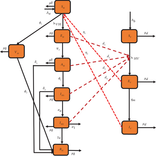
Parameter	Description
α	Biting rate of mosquitoes.
ϕ₁	Vaccination rate.
d₁, d₂, d₃, d₄	Modification parameters.
η₁, η₂	Modification parameters.
Λ_a	Recruitment rate of humans.
β₁	Transmission probability from mosquitoes to humans.
β₂	Transmission probability from humans to mosquitoes.
ψ_a	Transition rate from the exposed to the asymptomatic compartment.
ϕ_a	Transition rate from the asymptomatic to the mildly infected compartment.
σ_a	Transition rate from the mildly infected to the severely infected compartment.
γ_a	Recovery rate of the severely infected humans.
σ₁	Disease-induced death rate.
δ₁, δ₂	Recovery rate of the asymptomatic and mildly infected humans.
μ_δ	Death rate of humans.
Λ_b	Recruitment rate of mosquitoes.
q_m	Transition rate from the exposed mosquitoes to the infected compartment.
ϕ₂	Rate at which the vaccinated humans enter the recovery compartment.
μ_d	Death rate of mosquitoes.

λ_VH is the per-capita contact transmission rate from mosquitoes to humans given by

( )

λ_HV, the per-capita infection rate from humans to mosquitoes given by

( )

2.1. Model Analysis: Positivity and Boundedness

Theorem 1. Let {S_H, V_H, E_H, A_H, I_H1, I_H2, R_H, S_V, E_V, I_V} be the set of positive solution of the state Equation (1) with nonnegative parameters and initial condition given by {S_H ≥ 0, V_H ≥ 0, E_H ≥ 0, A_H ≥ 0, I_H1 ≥ 0, I_H2 ≥ 0, R_H ≥ 0, S_V ≥ 0, E_V ≥ 0, I_V ≥ 0}.

Proof 1. To prove the positivity of model Equation (1), we apply the method demonstrated in [41]. Thus, we let , Ω₀ = α(β₁η₁/N_H)E_V, Ω₁ = α(β₁η₂/N_H)I_V, Ω₂ = α(β₂d₁/N_H)E_H, Ω₃ = α(β₂d₂/N_H)A_H, Ω₄ = α(β₂d₃/N_H)I_H1, and Ω₅ = α(β₂d₄/N_H)I_H2.

Then, representing malaria model Equation (1) as a nonlinear differential equation, we get

(2)

where

( )

with ϱ₁ = (ϕ₁ + μ_δ), ϱ₂ = (ϕ₂ + μ_δ), ϱ₃ = (ψ_a + μ_δ), ϱ₄ = (ϕ_a + δ₁ + μ_δ), ϱ₅ = (δ₂ + σ_a + μ_δ), ϱ₆ = (γ_a + σ₁ + μ_δ), ϱ₇ = (q_m + μ_d), y₁ = (Ω₂ + Ω₃ + Ω₄ + Ω₅), and

( )

Now, from the vaccinated equation of model Equation (1), solving with the integrating factor method gives

( )

The asymptomatic equation of model Equation (1) also gives

( )

Further, solving the mildly infected equation of model Equation (1) with the integrating factor method gives

( )

Then, from the severely infected equation of model Equation (1), we get

( )

It follows that (d/dt)V_H ≥ 0, at t = 0, for V_H(0) = 0, (d/dt)A_H ≥ 0, at t = 0, for A_H(0) = 0, (d/dt)I_H1 ≥ 0, at t = 0, for I_H1(0) = 0, and (d/dt)I_H2 ≥ 0, at t = 0, for I_H2(0) = 0. Hence, from comparative analysis, the same can be concluded for the remaining state variables, S_H(t), I_H2(t), S_V(t), E_V(t), I_V(t), which guarantee the positivity of the state variables throughout the study. Hence, based on this assertion, we argue that the off-diagonal entries of matrix Q₁ are nonnegative and that of B ≥ 0. Hence, the malaria equation (1) is positively invariant in .

Theorem 2. The malaria model (1) has a nonnegative solution and bounded positively within the invariant region, ϖ ∈ R¹⁰;

( )

Proof 2. Let N_H(t) = S_H + V_H + E_H + A_H + I_H1 + I_H2 + R_H and N_V(t) = S_V + E_V + I_V. Then, we can deduce the following:

(3)

From (3), solving the equation related to humans gives

(4)

In addition, the vector-related equation of (3) becomes

(5)

Hence, it follows that (dN_H(t)/dt) ≤ 0 and (dN_V(t)/dt) ≤ 0 if N_H(0) ≥ (Λ_a/μ_δ) and N_V(0) ≥ (Λ_b/μ_d). Hence, the region given by ϖ is positive invariant. Further, N_H(0) > (Λ_a/μ_δ) and N_V(0) > (Λ_b/μ_d); then, the solution approaches ϖ in the final time, or N_H(t) and N_V(t) approach Λ_a/μ_δ and Λ_b/μ_d asymptotically. Hence, the region given by ϖ attracts all the solutions in .

3. Malaria-Free State and Computation of the Basic Reproduction Number

The

rate, one of the look-out threshold quantities, measures on average the infected individuals; an infected person has been infected throughout infectivity. The

rate above one insinuates that the number of cases is rising, and the below one rate means the epidemic is waning. As owned by Seidu, Makinde, and Asamoah [42], the subsection uses the recently developed novel algebraic technique to derive the

. Thus, considering the Malaria-free state given by

(6)

where

( )

The Jacobian matrix of the infected subsystem evaluated at the malaria-free fixed point is obtained as

( )

Following this method, the determinant of

can be rewritten as

, where

and

are the respective parts of the determinant containing infectivity/transmission terms and transition terms obtained as follows.

( )

Using Remark 3.1 of [42], the basic reproduction number of the model is obtained as

(7)

Upon substituting the point

into Equation (7), the

becomes

(8)

3.1. Local Stability Analysis of Malaria-Free State

Theorem 3. The Malaria-free point of model (1) is LAS when and unstable when .

Proof 3. The Malaria model (1) is linearized at to give the following results.

(9)

From (9), the first four eigenvalues are derived as Φ₁ = −μ_d, Φ₂ = −μ_d, Φ₃ = −ϱ₁, and Φ₄ = −ϱ₂. The eigenvalues that remain are derived by the submatrix S_M as follows:

(10)

Following the Routh–Hurwitz criterion [43, 44], submatrix S_M will have negative real eigenvalues if Tr(S_M) < 0 and Det > 0. Hence, from submatrix (S_M), it can be deduced that the trace Tr(S_M) = −(ϱ₃ + ϱ₄ + ϱ₅ + ϱ₆ + ϱ₇) < 0 and .

It follows from the above derivations that when , then all eigenvalues of submatrix (S_M) would have a negative real part. Hence, the malaria model (1) would be locally asymptotically stable at , but otherwise unstable.

3.2. Local Stability Analysis of Malaria-Present Equilibrium

The malaria-present equilibrium is a point with at least one nonzero infected state. The subsection determines

, representing the malaria-present steady states of model (1). Thus, the equations of the malaria model (1) are expressed in terms of the force of infection of the Malaria-present states as

( )

The subpopulations

are summed up to obtain

(11)

Now, with the force of infections given by

(12)

(13)

The malaria model (1) satisfies the following polynomial equation at the malaria-present point

(14)

where

( )

The polynomial Equation (14) is used to demonstrate the likelihood of multiple endemic equilibria even with . As observed, the coefficient Θ₀ always remains nonnegative for nonnegative parameter values, and Θ₂ will be nonpositive when . Hence, the underlying theorem holds.

Theorem 4. The malaria model (1) has

D1: a unique endemic steady-state point if ;

D2: a unique endemic steady-state if Θ₂ < 0, and either Θ₂ = 0 or ;

D3: two endemic steady states if Θ₂ > 0, Θ₁ < 0 and ;

D4: no endemic steady state otherwise.

The discourse from Theorem 4 implies the following. In [D1], the malaria model (1) has a unique endemic state when . Further, [D3] indicates a backward bifurcation possibility. Thus, the coexistence of the disease-free and endemic steady states when . Backward bifurcation implies that is an insufficient condition to eliminate the disease. Following the investigation, the mitigation of the disease would be challenging unless much effort and better intervention measures are applied. To confirm backward bifurcation possibility in malaria model (1), we let the discriminant and derive the critical value of , denoted by . The derivation results in , which confirms the following theorem.

Theorem 5. The malaria model (1) exhibits backward bifurcation when [D3] of Theorem 4 holds, resulting in .

3.3. Global Stability Analysis of Malaria-Free State

Consider the malaria model system (1). If the model system (1) is globally asymptotically stable at the malaria-free point

, then the system will always remain stable at

and the disease will not persist, regardless of the amount of the perturbation. The subsection would investigate the Castillo-Chavez approach, which has been shown in the research of [41, 45], to study the global asymptotic stability of the malaria model at the malaria-free equilibrium. The analysis is presented as follows:

(15)

(16)

with χ₁ representing the population of uninfected. Thus, χ₁ = (S_H, V_H, R_H, S_V), and χ₂ denotes the infected, with χ₂ = (E_H, A_H, I_H1, I_H2, E_V, I_V). The disease-free state of model system (1) is given by

Hence, the point is a globally asymptotically stable equilibrium for the model (1) if the following criteria are satisfied.

(Z₁) Given dχ₁/dt = h₁(χ₁, 0), is GAS.

(Z₂), where for (χ₁, χ₂) ∈ ζ.

Theorem 6. The point is GAS whenever .

Proof 4. The model system (1) is considered to derive h₁(χ₁, χ₂) and h₂(χ₁, χ₂) as

( )

First, to prove condition Z₁, the system dχ₁/dt = h₁(χ₁, 0) is structured as follows:

(17)

which gives

( )

and

(18)

In addition,

(19)

Solving Equation (19) gives

(20)

Now, from (18), as t⟶∞,

(21)

which implies the convergence of

. Hence,

is GAS, which verifies condition one. What happens next is that the assessment of condition (Z₂) is done with

. Thus, we have

(22)

Hence, is derived as follows:

( )

From model Equation (1), it can be confirmed that the population of the humans is bounded by and that of the vector by . Hence, , , , , and which implies that is positive definite. It can also be noted that is an M-matrix with the off-diagonal entries nonnegative. Hence, the requirement of the two conditions is met, which is proof of the global asymptotic stability of .

3.4. Global Stability Analysis of Malaria-Present State

The subsection is geared towards determining the global dynamic behaviour of model (1) at the malaria-present state.

Theorem 7. With , the malaria-present point of model system (1) is GAS, otherwise unstable.

Proof 5. In the study of [46], we refer to Theorem 5 and Lemma 3 and Lemma 4 to deduce the GAS of model (1) at the malaria-present state . We let (S_H, E_H, A_H) represent the subsystem of model (1) as follows:

(23)

Now, the Jacobian of submatrix (23) is derived as follows:

( )

Let

g₁ = −ϕ₁ − μ_δ − αβ₁(η₁E_V + η₂I_V/N_H), g₂ = αβ₁(η₁E_V + η₂I_V/N_H)

It follows that the second additive matrix, , becomes

( )

Now, the function P(y) = (S_H, E_H, A_H) is derived as P(y) = diag{1, E_H/A_H, E_H/A_H}, and P(y)^−′ = diag{1, A_H/E_H, A_H/E_H}. Hence, the rate of change of P_f(y) is given by and .

Further,

( )

Hence, matrix is derived as follows:

( )

where

ρ₁₁ = g₁ − ϱ₃, ,

Now, let Y = (Y₁, Y₂, Y₃) be a vector in R³, with its norm ‖•‖ given by ‖Y‖ = max{|Y₁|, |Y₂|, |Y₃|}. Let be a Lozinki measure with respect to ‖Y‖. Then, the approximating method as in [47] is applied such that , where sup{z₁, z₂} = sup{L(ρ₁₁) + |ρ₁₂|, L(ρ₂₂) + |ρ₂₁|} and |ρ₁₂|, |ρ₂₁| denote matrix norms with respect to the vector norm L₁. L also denotes the Lozinki measure concerning the L₁. Then,

( )

Hence, . It follows from Equation (23) that

( )

Now,

(24)

Following the above deductions, Equation (24) is put into (25) below.

(25)

Hence,

(26)

(27)

It follows from (27) that the subsystem (23) is GAS around the interior point of . Hence, for the remaining subsystem of (1) given below,

(28)

When the subsystem (28) is solved with the initial conditions of V_H(0), , , R_H(0), S_V(0), E_V(0), and I_V(0), then as t⟶∞, , , , , , , and . Hence, the GAS of the endemic point is ascertained.

3.5. Sensitivity Analysis

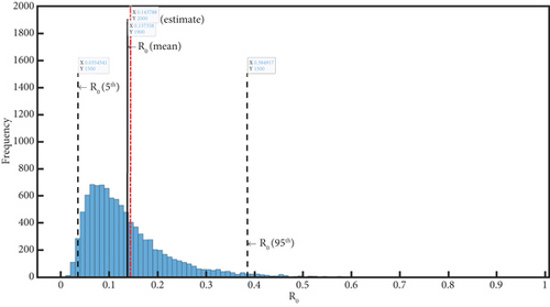
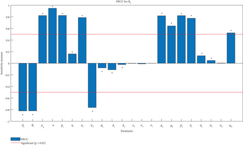
The , known to be one of the essential threshold quantities, is associated with many parameters which are susceptible to change. Owing to the susceptibility of these parameters, sensitivity analysis becomes inevitable in epidemiological modelling as it sheds light on which parameters significantly affect the and needs to be worked on. The susceptibility in the model parameters that are directly involved in the computation of the creates variability in the estimate of . However, the statistical methods—the Latin hypercube sampling (LHS) and partial rank correlation coefficient (PRCC)—are considered to assess the variability in the (see [48, 49]). With a MATLAB simulation, the method enables us to dive into the variability analysis of the malaria model (1) parameter. For the of Malaria model (1) given by Equation (7), the LHS quantifies the magnitude of the influence of the parameters, and by the PRCC, we find influential parameters by their computed values. By considering a 1000 sample, the LHS analyses the uncertainty of as displayed by the histogram in Figure 2. From Figure 2, the uncertainty in is exhibited by the histogram with the uncertainty computed using a 95% confidence interval as shown by the broken lines. The distribution depicts the estimated values of , the mean, and 5th and 95th percentiles, respectively, simulated as 0.143788, 0.01545, 0.41491. Generally, the distribution of becomes widely spread with higher uncertainty. Figure 3 is the PRCC diagram, and it displays the sensitivity of to the considered model parameters of the malaria model (1). From the simulation of the PRCC, the most crucial parameters are those with significantly small p value (p ≤ 0.005) and big PRCC value, as it indicates a stronger relationship between the parameters. The PRCC-generated findings of Figure 3 showed that the parameters μ_δ, α, β₁, η₁, η₂, Λ_b, μ_d, β₂, d₁, d₂, d₃, d₄ and q_m have PRCC bars in a positive direction. These parameters exert to some extent a certain amount of influence on the . However, the parameters with the most significant influence are the ones with their bars exceeding the threshold marked by the red bar. The significance of decreasing the values of the parameters with high positive bars is that it decreases the , bringing it down to less than one. Also, the parameters Λ_a, ϕ₁, ψ_a, ϕ_a, δ₁, δ₂, γ_a, σ_a have PRCC bars in a negative direction, which means when their values are increased, they will help lower the . Hence, the interventions should aim at lowering the positive PRCC parameter values and increase the parameters Λ_a, ϕ₁, ψ_a, ϕ_a, δ₁, δ₂, γ_a, σ_a.

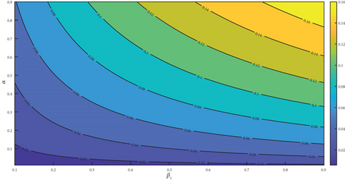
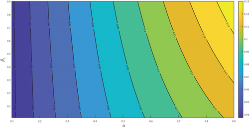
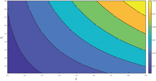
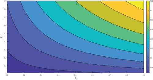
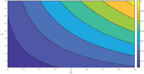
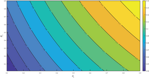
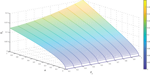
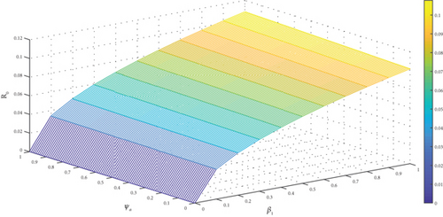
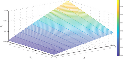
The observation of Figures 4(a), 4(b), 4(c), 4(d), 4(e), and 4(f) showed a positive effect of the identified parameters on . Hence, increasing awareness to prevent mosquito bites through the use of treated bednet, spraying the environment to reduce drastically the mosquito population with insecticide spray, and adhering to pharmaceutical interventions such as seeking early medical attention at the early onset of the disease and implementation of effective vaccination programs would reduce . Furthermore, the analysis was carried further by generating a 3D plot for some selected parameters. The generated figure of Figure 5(a) showed that increasing the value of α from zero to one increases the , but the remains the same even if μ_δ is increased from zero to one. From Figure 5(b), we noticed that as β₁ increased from zero to 1, the increases. But remains the same as ψ_a increased from zero to one. Lastly, we observed from Figure 5(c) that as β₂ increases from zero to one, it causes to increase but remains the same when ψ_a is increased from zero to one.

3.6. Bifurcation

Over time, it has become established that

guarantees the eradication of diseases. This claim, however, has been refuted by several recent epidemiological studies that involve backward bifurcation. The phenomena in several disease modelling research have demonstrated the potential for the disease to persist even in the presence of stable disease-free equilibrium and

. A stable disease-free and endemic equilibrium coexisting in the system contributes to the disease’s persistence. Backward bifurcation has a significant negative impact on disease control since it would need a more aggressive strategy to bring the mathematical

when the illness starts to spread. The subsection explores the possibility of backward bifurcation in model system (1), by exploring the theory of central manifold as applied in [50]. Thus, suppose

is considered as the bifurcation parameter, then from (7),

becomes

(29)

Now, following matrix (9), the right eigenvector

is given by

( )

with

( )

In addition, matrix (9) has a left eigenvector v = (v₁, v₂, ⋯, v₁₀), which satisfies the condition v.w = 1, where

( )

Following Theorem 4.1 in [50], the nonzero partial derivatives in relation to the equation a and b given by

(30)

and

(31)

are derived as follows:

( )

Hence,

( )

Now, it follows that deriving b using Equation (31), we get

( )

Thus,

( )

From the computations, b is positive as conventionally the case. The result of a determines the dynamics of the malaria model (1) around . From [50], the malaria model (1) will undergo forward bifurcation when a is negative and backward bifurcation when a is positive.

3.7. Vaccine Effect Assessment

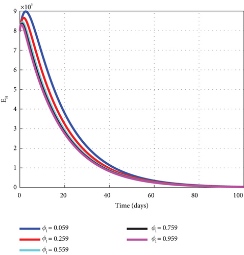
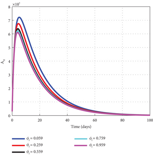
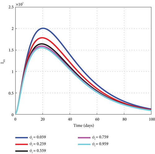
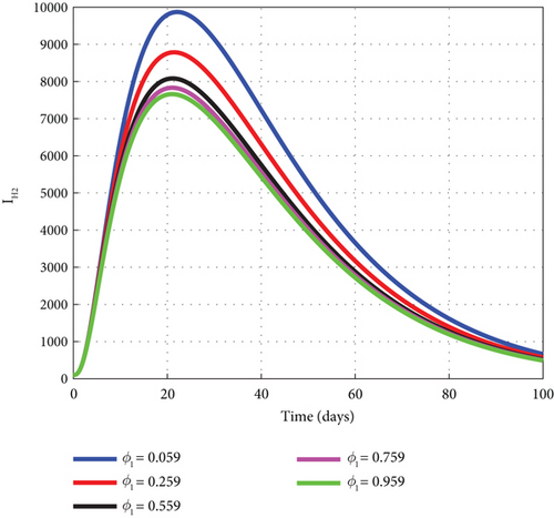
As mentioned in the proceeding objective, the impact of vaccines on the malaria disease dynamics is assessed by conducting a comprehensive analysis using MATLAB 18 to generate graphs for a detailed study. The simulated plot of the graphs revealed that increasing the vaccination parameter ϕ₁ reduces the number of the exposed, asymptomatic, mildly, and severely infected humans. As noted in Figures 6(a), 6(b), 6(c), and 6(d), when the dose of the vaccination rate ϕ₁ increasingly takes the set of values of 0.059, 0.259, 0.559, 0.759, and 0.959, it decreases the exposed, asymptomatic, mildly, and severely infected human cases. The analysis indicates that vaccines hold substantial public health implications by shifting the classical understanding of nonpharmaceutical preventive malaria control such as insecticide net usage and spraying the environment to control the vector to the pharmaceutical measure of vaccines.

4. The Intervention Model Development

The section determines intervention for the malaria model (1) that would halt the transmission of the disease. The triplet interventions (u₁(t), u₂(t), u₃(t)) are identified such that

•
u₁(t) is the bednet usage of the susceptible human to derive protection from a mosquito bite.
•
u₂(t) is the treatment of the infected humans.
•
u₃(t) is the elimination intervention of the vector through insecticide spray.

With the intervention of (u₁(t), u₂(t), u₃(t)) identified for the malaria model (1), the structured nonautonomous malaria intervention model becomes

(32)

The target of intervention model (32) is to minimize the number of infected human compartments and eradicate the various phases of the vector while minimizing the expense associated with putting the identified interventions into practice. As a result, the objective functional (33) is minimized under the constraints of (32), a nonautonomous equation.

(33)

Equation (33) integrand has coefficients of the state variables which serve as balancing coefficients that measure the intervention cost on the interval [0, T]. We seek an optimal control u_i, for i = 1, ⋯, 3 such that

(34)

In connection with minimizing the objective functional (33) to the model system (32), the Pontryagin maximum principle [51] converts the (33) and (32) into a minimization problem and finds its solution. We let denote the state variable and u₁(t), u₂(t) and u₃(t) the related controls. The existence of an optimal control problem is shown as follows:

System (32) is structured into the form

(35)

where

( )

and

( )

Considering Equation (35), |G₂(u, X₁) − G₂(u, X₂)| becomes

(36)

and

(37)

Following Equations (36) and (37), the entire system K(X) = G₁X + G₂(u, X) is given by

( )

Hence,

( )

It follows that A is a nonnegative constant which is independent of the state variable such that

( )

where

( )

Furthermore, |K(X₁) − K(X₂)| ≤ Γ|K₁ − K₂|, with Γ = max{J, ‖L‖} < ∞. Therefore, A(K) is uniformly Lipschitz continuous. Hence, the malaria model (1) has a solution that exists.

Now the method [51] is applied which converts the malaria model (1) and (33) into the minimization of subject to u₁, u₂, u₃.

Theorem 8. Suppose condition (34) is satisfied by the control triplets u_i, for, i = 1, ⋯, 3, then the adjoint variable φ_j exists which satisfy the underlying adjoint system;

(38)

with transversality conditions

(39)

(40)

where

( )

(41)

Proof 6. The Hamiltonian (42) given by

(42)

is explored to deduce the adjoint system (38). We partially differentiate (42) subject to the state variables given by

( )

The controls u_i, for, i = 1, ⋯, 3 are characterised as presented in the given equation:

(43)

Using standard argument, the characterization is done by employing bounds such as

(44)

4.1. Numerical Simulation

With the aid of numerical examples to complement the analytic analysis, the method, forward-backwards sweep, propounded by [52] is applied to generate simulated graphs of the malaria model (32). The optimality control simulated graphs are compared to the noncontrol graph for comparative analysis to be made. To understand the dynamics of the control strategies on the model, we explored the scenario of pairing different strategies to assess their impact on mitigating the spread of the epidemic. The simulated graphs were generated with the widely known scheme, and the fourth order Runge–Kutta was employed to solve the numerical model’s (32) optimality system. The scheme solves the adjoint system (38) backwards in time and system (32) forward in time. With a specified interval t ∈ [0,100], chosen initial conditions and the parameter values of Table 2, the iterative scheme solves the optimality system, considering the associated transversality condition. Further, the coefficients of the state variable targeted for minimizing in the objective functional (33) are chosen arbitrarily as H₁ = H₂ = H₃ = H₄ = H₅ = 10, h₁ = 5, h₂ = 10, and h₃ = 8. h₂ which represents the treatment intervention is considered to be greater than h₁ and h₃ since it involves diagnosis and treatment cost. Further, h₃ is assumed to be greater than h₁ since it may involve the cost of insecticide and spraying.

Table 2. Model 1: parameters and source with days as time.

Parameter	Values	Source	Parameter	Values	Source
a	(0.0696,0.5)	[20, 39, 53]	ϕ_a	0.31	Assumed
ϕ₁	(0.01,0.1)	[39]	σ_a	0.03	Assumed
d₁, d₂, d₃, d₄	(0.1,1)	[37, 54]	γ_a	0.4071	Assumed
η₁, η₂	(0.01,0.1)	[20, 54]	σ₁	(0.0004,0.2)	[39, 55]
Λ_a	(100, 1000)	[20]	δ₁, δ₂	(0.01,1)	[20]
β₁	(0.021,0.6)	[24, 54, 56]	μ_δ	0.0000548	[37]
β₂	(0.1,0.5)	[24, 54, 56]	Λ_b	50	[57]
ψ_a	0.06	[57]	q_m	0.27	[58]
ϕ₂	0.15	Assumed	μ_d	(0.05,0.3)	[22, 39, 58]

4.2. A: The Intervention of u₁ and u₂

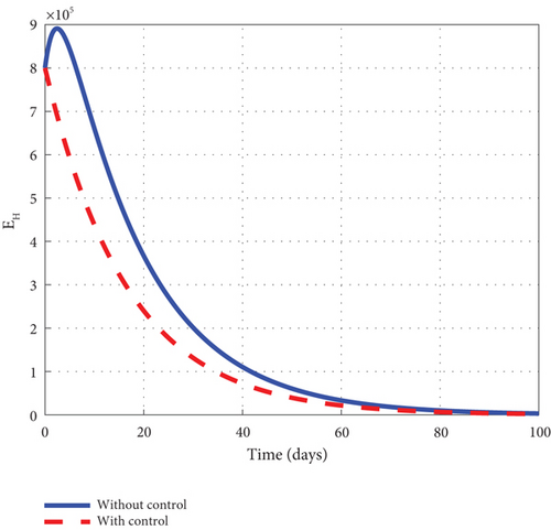
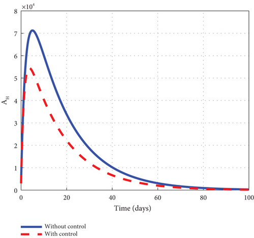
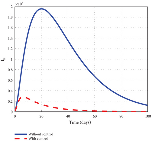
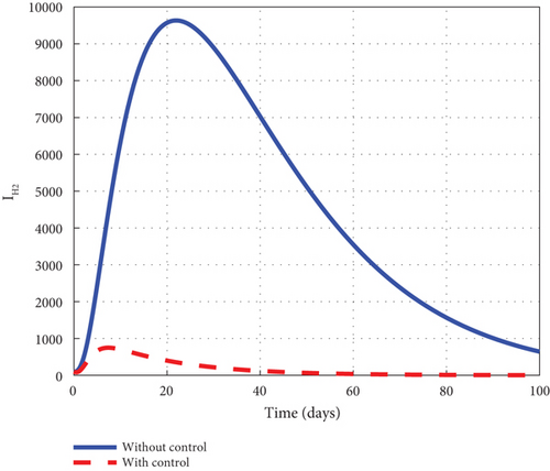
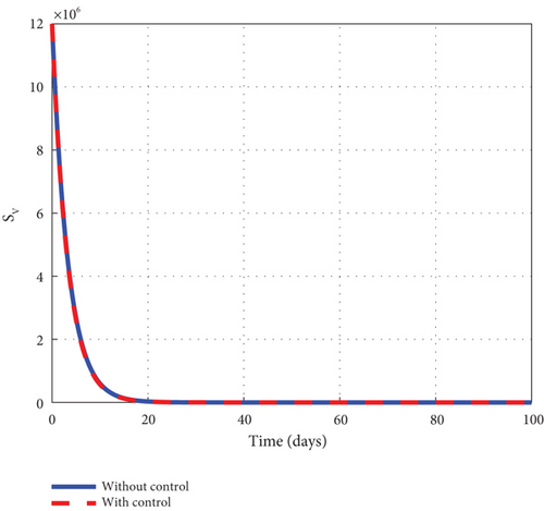
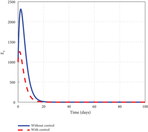
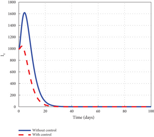
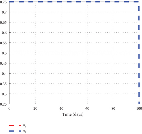
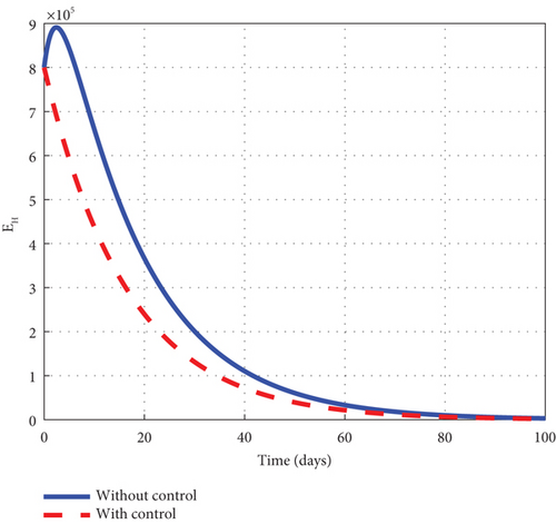
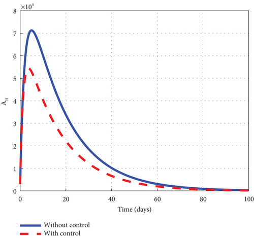
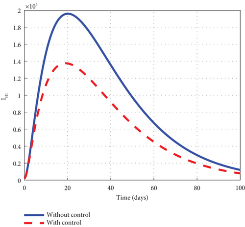
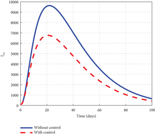
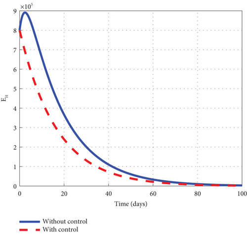
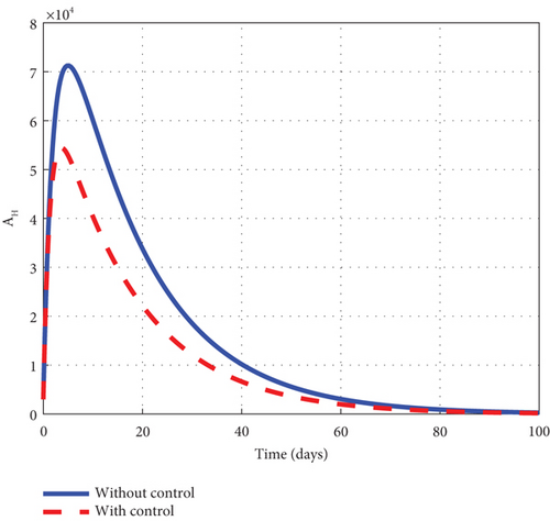
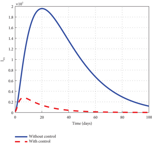
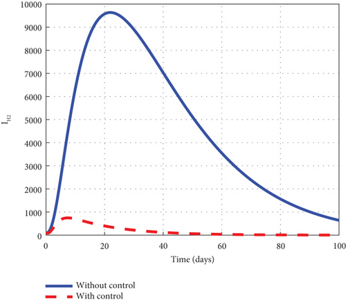
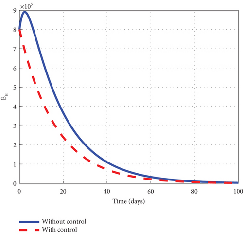
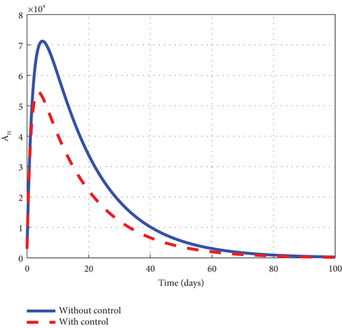
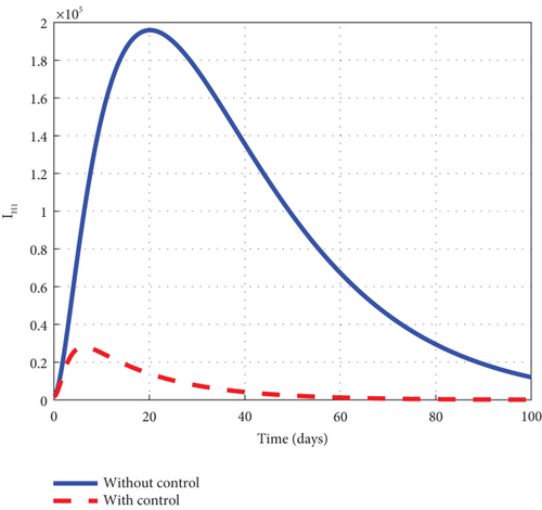
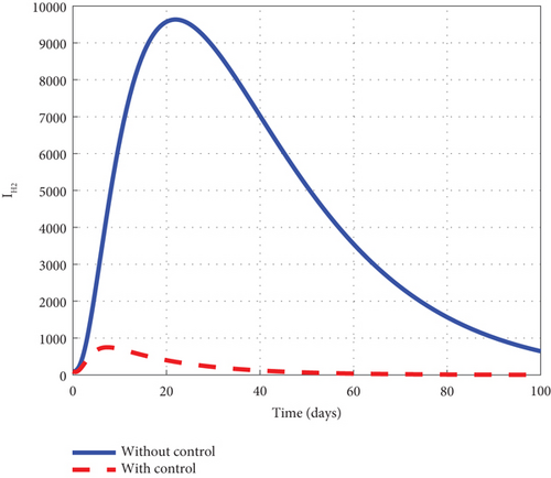
To advance our understanding of the dynamics of the malaria model (1), the interventions of u₁ and u₂ are considered to generate graphical solutions of the control model (32) and a comparative analysis is made with the noncontrol model (1). From the analysis, we noted that the exposed human’s noncontrol graph of Figure 7(a) quickly rises in the early days to 8.8 × 10⁵ in 3 days and gradually decreased and wiped out of the population in 90 days. The noncontrol asymptomatic human’s graphs of Figure 7(b) rocketed to 6.9 × 10⁴ in 5 days and swiftly lowered as it degenerated from the population in 90 days. The mildly infected human’s graph of Figure 7(c) was picked from zero and gently moved to 17.6 × 10⁴ in 18 days. It then changed its course and began to decline smoothly to 0.8 × 10⁴ in 100 days. The severely infected noncontrol human’s graph of Figure 7(d) gently moved from zero to 8.7 × 10³ in 20 days and smoothly lowered afterwards to 0.8 × 10³ in 100 days. The susceptible mosquito graph of Figure 7(e) declined speedily to zero in 20 days. The noncontrol exposed mosquito graph of Figure 7(f) swiftly increased from 1.0 × 10⁵³ to 2.5 × 10³ in 2 days and then quickly dropped to zero in 20 days. The infected graph of Figure 7(g) steadily picked from 1.0 × 10³ to 1.36 × 10³ in 5 days and sharply decreased to zero in 30 days. The control-generated graphs of the intervention of u₁ and u₂ produced the desired results. The exposed human graph slowly decreased from 8.0 × 10⁵ to zero in 100 days but stayed below the noncontrol graph. The asymptomatic depicted a similar pattern but lay below the noncontrol throughout the simulated time. The mildly infected control human’s graph took the same pattern but could only raise a little about 2.0 × 10⁴. The graph slowly lowered from that level and decreased to zero in 60 days. The severely infected control human’s graph depicted the noncontrol graph and slowly raised to 0.8 × 10³ in the early days but became greatly minimized afterwards. The control susceptible mosquito graph reached equilibrium with the noncontrol and lowered in the same pattern to zero in 20 days. The exposed mosquito control graph mimicked the noncontrol and raised gently to 1.3 × 10³ in 2 days but gradually lowered to zero after day 2. The control infected mosquito graph dropped gently from 1.0 × 10³ to 9.30 × 10² in 2 days and gradually decreased to zero in 30 days depicting the noncontrol graph as observed in graphs of Figure 7. Figure 7(h) is the control profile plot generated using intervention u₁ and u₂. From the graph, we observed that both u₁ and u₂ stayed on the top bound till 100 days when they dropped to the lower bound.

4.3. B: The Intervention of u₁ and u₃

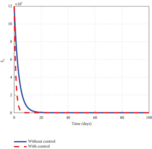
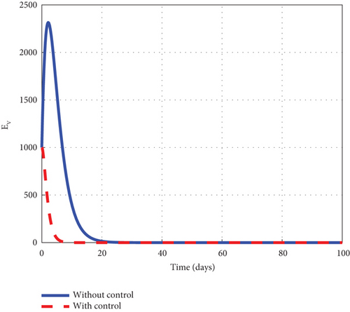
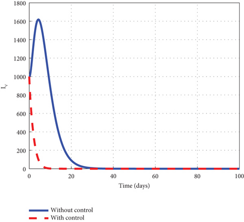
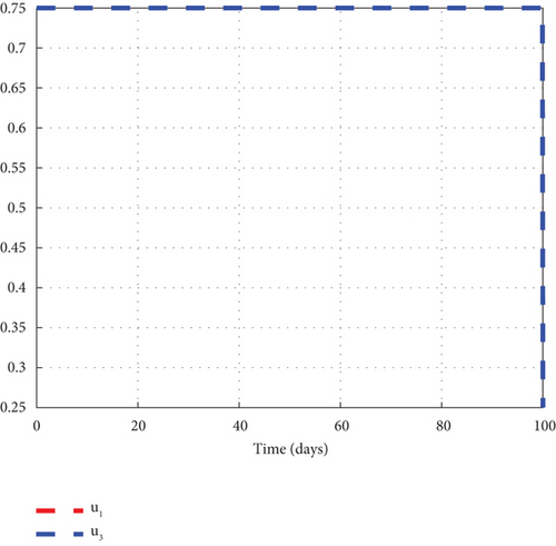
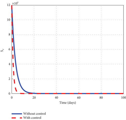
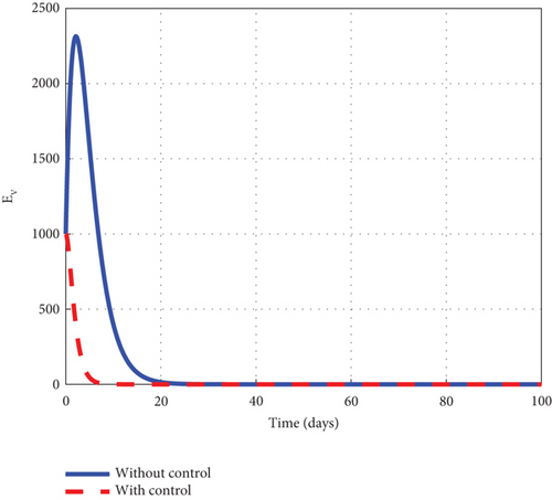
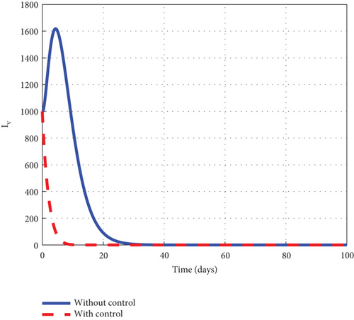
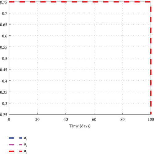
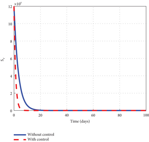
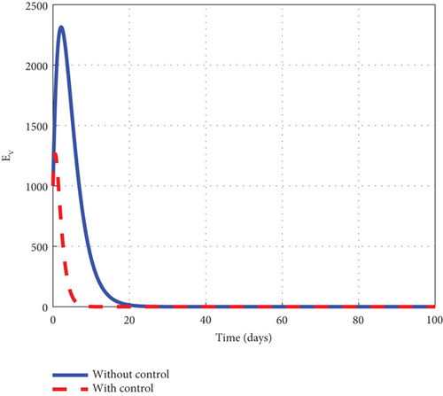
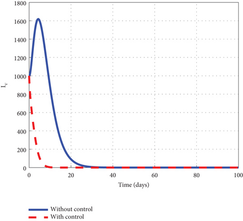
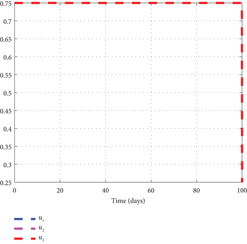
The intervention of u₁ and u₃ is considered to provide detailed information on the dynamics of the control model (32) generated solution to the noncontrol solution. We observed from the simulated plots that the noncontrol exposed human’s graph of Figure 8(a) rose quickly to 8.8 × 10⁵ in the first 3 days and fell smoothly afterwards to zero in 90 days. The asymptomatic human’s graph of Figure 8(b) soured from 0.3 × 10⁴ to 6.9 × 10⁴ in 5 days and slowly declined to zero in 90 days. The noncontrol mildly infected human’s graph of Figure 8(c) smoothly picked from zero and soured to 17.6 × 10⁴ in 18 days. The dynamic behaviour of the graph changed after 18 days, and it began to decrease gradually to 0.8 × 10⁴ at the final time. The severely infected human’s graph of Figure 8(d) moved from zero to 8500 in 20 days and fell through to 450 at the final simulated time. The susceptible noncontrol mosquito graph of Figure 8(e) continuously declined from 12 × 10⁶ to zero in 10 days and remained there for the rest of the simulated time. The exposed noncontrol graph of Figure 8(f) steadily rose early to plummet to 2500 in 3 days. The graph then decreased speedily to zero in 25 days and stayed there for the rest of the simulated time. The infected mosquito graph of Figure 8(g) rose to 1350 in 5 days and then fell to zero in 30 days. However, with the intervention of u₁ and u₃, different dynamic behaviour was obtained. The intervention caused the control exposed graph to decrease from 12 × 10⁶ to zero in 80 days, but the graph stayed below the noncontrol graph throughout the simulated time. The asymptomatic control human’s graph mimicked the noncontrol graph but stayed below it. The mildly infected control human’s graph, taking the same pattern as the noncontrol moved from zero to 12.3 × 10⁴ in 18 days. It then decreased slowly to 0.8 × 10⁴ at the final simulated time. The severely infected control graph depicted the noncontrol graph and moved from zero to 6000 in 20 days. The graph proceeded after 20 days and dropped slowly to 300 at the final time. The control susceptible graph dropped sharply to hit zero in 8 days and stayed there for the remaining time. Further, the control exposed graph quickly fell from 1000 to zero in 8 days, staying below the noncontrol graph. The control infected graph swiftly dropped from 1000 to zero in 8 days, remaining below the noncontrol graph as seen in the graphs of Figure 8. Finally, Figure 8(h) is the control profile plot generated using intervention of u₁ and u₃. From the graph, u₁ and u₃ both stayed in the upper limit until 100 days when it dropped to the lower limit.

4.4. C: The Intervention of u₂ and u₃

A comparative analysis involving the intervention of the control u₂ and u₃ of the control model (32) to the noncontrol model (1) is made to elucidate the dynamic behaviour of the disease. The investigation indicated that the exposed noncontrol human’s graph of Figure 9(a) rose steadily in the early days to 8.8 × 10⁵ and decreased gradually until it entirely seemed to have been wiped out of the population at the final time. The asymptomatic noncontrol graph of Figure 9(b) swiftly raised to 6.9 × 10⁴ in 5 days and changed its direction to fall gradually to zero in 100 days. The mildly infected noncontrol graph of Figure 9(c) moved from zero to 17.5 × 10⁴ in 18 days and then decreased gradually to 0.9 × 10⁴ at the final time. The severely infected noncontrol graph of Figure 9(d) picked from zero and steadily increased to 8500 in 20 days. The graph then decreased gradually to 400 at the final simulated time. The susceptible noncontrol mosquito graph of Figure 9(e) dropped from 12 × 10⁶ to zero in 20 days and remained there for the rest of the simulated time. The exposed noncontrol mosquito graph of Figure 9(f) sharply rose from 1000 to 2500 in 3 days and suddenly fell to zero in 20 days. The infected noncontrol mosquito graph of Figure 9(g) picked from 1000 to 1350 in 5 days and then lowered gradually till it hit zero in 30 days. The execution of the intervention of the control u₂ and u₃ generated graphs with different dynamic behaviour. The control exposed human graph decreased right from 8.0 × 10⁵ and progressed steadily to zero at the final time. The control asymptomatic human graph took a similar pattern as the noncontrol and increased from 0.3 × 10⁴ to 5.3 × 10⁴ in 5 days. The graph changed its dynamic behaviour and lowered gradually after 5 days to zero but stayed below the noncontrol graph for the simulated time. The mildly controlled infected human graph slightly increased similarly to the noncontrol graph but was greatly minimized. In addition, the severely controlled infected human graph depicted the noncontrol and increased for the 5 days and declined afterwards. The control susceptible mosquito graph dropped sharply in the first 20 to meet the noncontrol and maintained that level for the simulated time. The control exposed mosquito graph took the same pattern as the noncontrol but declined sharply to hit zero at 6. The control infected mosquito graph dropped swiftly from 1000 to zero in 10 days as noticed in the graphs of Figure 9. Figure 9(h) is the control profile of the model using the intervention of u₂ and u₃. The result of the graph and the intervention of u₂ and u₃ should not be relaxed for the entire simulated time.

4.5. D: The Intervention of u₁, u₂, and u₃

Finally, to further boost management decision-makers with an advanced understanding of the malaria 1 disease’s dynamics, we employed all three interventions of the control model (32) and circumspectly experimented with them to generate simulated plots to support the analytic investigation. From the simulation, we observe that the noncontrol exposed human’s graph of Figure 10(a) slightly increased from 8.0 × 10⁵ to 8.8 × 10⁵ in 3 days and gradually lowered after 3 days to zero at the final time. The asymptomatic noncontrol human’s graph of Figure 10(b) steadily raised from 0.4 × 10⁴ to 6.9 × 10⁴ in 5 days and slowly declined to zero at the end of the simulated time. The mildly infected noncontrol graph of Figure 10(c) increased from zero to 17.5 × 10⁴ in 18 days and then reduced gradually to 0.8 × 10⁴ at the final time. The severely infected noncontrol human’s graph of Figure 10(d) continuously increased from zero to 8500 in 20 days and dropped slowly to 400 at the final time. The susceptible noncontrol mosquito graph of Figure 10(e) dropped speedily to zero in 20 days from 12 × 10⁶ and maintained that level for the remaining time. The exposed noncontrol mosquito graph of Figure 10(f) sharply increased from 1000 to 2500 in 3 days and then swiftly dropped to zero in 20 days. It then stayed at zero for the remaining time. The noncontrol infected mosquito graph of Figure 10(g) moved from 1000 to 1350 in 5 days and then changed the dynamics and began to decrease. The graph progressed from 1350 to zero within 25 days. The intervention of u₁, u₂, and u₃ reverted the dynamic behaviour of the disease. We noted that the control exposed human’s graph decreased right from day 1 and progressed steadfastly to zero in 100 days. The control asymptomatic graph mimicked the noncontrol graph and moved from 0.4 × 10⁴ to 4.4 × 10⁴ in 3 days, and then gradually decreased to zero in 100 days. The mildly infected control human’s graph depicted the behaviour of the noncontrol graph and slowly decreased to zero in 100 days. The severely infected control human’s graph moves slightly to 500 in 5 days and gently decreases to zero in 100 days. The control susceptible mosquito graph declined sharply in the first 5 days to zero and maintained the level for the simulated time. The control exposed mosquito graph dropped from 1000 to zero in 8 days and stayed there for the related time. The control infected mosquito graph swiftly dropped from 100 to zero in 8 days and stayed at that level to meet the noncontrol graph t = 30 as depicted by the graphs of Figure 10. Figure 10(h) is the control profile diagram generated using the three controls. From the graph, we observed that the three controls remained at the upper limit before dropping to the lower limit at the final time.

5. Cost-Effective Analysis

Cost-effective analysis is a method used to determine which among the available interventions is the most cost-effective in terms of achieving the desired outcomes. The analysis is conducted to let decision-makers make informed decisions about which interventions or treatments to prioritize based on their budget and desired outcomes. By the cost-effective analysis, we can determine the cost-effectiveness of each considered intervention by comparing the costs and outcomes [59–62]. The section engages the method of ACER (average cost-effectiveness ratio) and ICER (incremental cost-effectiveness ratio) to make a judgment of the most cost-effective intervention of the proposed interventions to tackle the malaria epidemic by comparing the costs and performances of the interventions. The ACER gives the total cost of an intervention to the prevented infections by the intervention. Further, considering two interventions of p₁ and p₂, the ICER is the difference in cost of p₁ and p₂ to the difference in the infection prevented by the intervention. Thus,

(45)

Table 3 provides the infections prevented by the named interventions ranked in increasing order of magnitude.

Table 3. Infections prevented in order of increasing magnitude.

Intervention	Total infection averted (×10⁷)	Total cost (×10³)	ACER	ICER
B	35343	3.6579	1.035 × 10⁻⁸	1.035 × 10⁻⁸
A	40727	4.2199	1.036 × 10⁻⁸	1.044 × 10⁻⁸
C	40786	5.0625	1.241 × 10⁻⁸	1.428 × 10⁻⁶
D	40803	6.4702	1.586 × 10⁻⁸	8.280 × 10⁻⁶

To find the most cost-effective intervention, a comparative analysis of the ACER’s values of the interventions must be made. The intervention with the least ACER value is the most cost-effective. By inspection, intervention B is the most cost-effective intervention. However, intervention D has the biggest ACER value, making it the least cost-effective intervention. But to decide on which intervention to discard, further detailed analysis needs to be carried out. Hence, we compute the ICERs of the interventions for further probing. From the ICER computations, we observe that intervention D has the biggest ICER value. Hence, it is discarded from the table and further analysis is made on the remaining interventions. The underlying analyses are made in Table 4

Table 4. Infections prevented in order of magnitude of interventions B, A, and C.

Intervention	Total infection averted (×10⁷)	Total cost (×10³)	ICER
B	35343	3.6579	1.035 × 10⁻⁸
A	40727	4.2199	1.044 × 10⁻⁸
C	40786	5.0625	1.428 × 10⁻⁶

Now, a further dive into the analysis from Table 4 shows that intervention A has the biggest ICER value than B. Hence, intervention A is deleted from the entries of Table 4. It follows that a new table is constructed in that regard.

Following the computation in Table 5, we deduce that intervention C has a bigger ICER value than B. Hence, we delete intervention C from Table 5. B therefore is the most cost-effective intervention, providing the optimum performance with the least cost.

Table 5. Infections prevented in order of magnitude of interventions B and C.

Intervention	Total infection averted (×10⁷)	Total cost (×10³)	ICER
B	35343	3.6579	1.035 × 10⁻⁸
C	40786	5.0625	1.428 × 10⁻⁶

6. Conclusion

The research studied a nonlinear differential equation malaria model to assess the impact of vaccines on the control of the disease. The research analysed the model and characterized its properties of positivity and boundedness. The asymptotic dynamic behaviour of the disease at the model’s equilibria was studied. Further, bifurcation analysis was conducted to study the local dynamic behaviour of the malaria model (1) at the malaria-free equilibrium. The investigation indicated that malaria model (1) exhibits forward bifurcation. Further, with the model’s input and initial conditions, sensitivity analysis was investigated to quantify the amount of influence each parameter has on . The influences of α, β₁, β₂, ψ_a and μ_δ on are depicted in Figure 5. We observe that the changes with a change in any of the given parameters. From Figure 5(a), we note that when α is significantly small, the disease can be mitigated even when μ_δ = 1. However, when α ≥ 1, the disease cannot be mitigated with μ_δ ≤ 0.1. In Figure 5(b), we see that the disease can be mitigated when β₁ is small. Thus, when β₁ is small, irrespective of the value of ψ_a, the disease could be eliminated. In addition, we observe in Figure 5(c) that the influence of β₂ on is great. Thus when ψ_a ≥ 1, the disease can be eliminated when β₂ is small. But when β₂ is big, the disease cannot be mitigated. Hence, α, β₁, and β₂ have a greater influence on the , and minimizing them would be a prudent initiative by stakeholders. Furthermore, the variability in was assessed by the LHS-PRCC. With the method, the uncertainty in is computed with a 95% confidence interval, with the mean, and 5th and 95th percentiles, respectively, simulated as 0.143788, 0.01545, and 0.41491. In addition, the bifurcation type invoked at the disease-free state is analysed and the result revealed that the convention that is the condition for eradicating the disease is not always sufficient when the system undergoes backward bifurcation. The presence of backward bifurcation means that the system is characterized by a coexistence of stable endemic and disease-free equilibria even when . In such circumstances, the infection needs to be dealt with at the early stages else it becomes difficult to control once the transmission begins to get out of control. Moreover, we formulated an intervention model to assess the respective effects of the various pairings of interventions on the dynamics of the disease. Lastly, an intervention cost analysis was conducted to identify the most cost-effective intervention regarding rewarding the desired outcome. From the analysis, intervention B was found to be the most cost-effective intervention. As recommended by the cost analysis, public health, in their effort to mitigate malaria in our communities, should target advocating and making insecticide nets available to the communities for easy access. In addition, areas in the community which serve as a hiding place for the vector should be targeted for spraying to control the vector. Furthermore, as confirmed by the vaccine analysis in Subsection 3.7, vaccines can assist in closing the gap that has not been fixed by the existing interventions. In addition, vaccines can help minimize the overall disease burden and incidence, hospitalization, and death from the disease especially in children. Hence, a vaccination program with a proper awareness strategy should be carried out by stakeholders to inform the public of the benefits of malaria vaccination. Lastly, vaccine availability should be 100% at all communities marked by the public health as areas of high malaria incidence to help foster smooth vaccination activities in these areas.

6.1. Strengths and Limitations of the Study

The research studied the asymptotic behaviour of malaria at the model equilibria. The bifurcation type invoked at the disease-free point is analysed as the classical understanding that is the condition for eradicating the disease is not always sufficient when the system undergoes backward bifurcation. The study analysed the global sensitivity to quantify the influence each parameter related to the has on it. The model was redesigned into an intervention model for public health benefit with an insight shed on the shift from the classical understanding of nonpharmaceutical preventive malaria control to pharmaceutical measures of vaccines. A cost analysis of the intervention model was examined to identify the most cost-effective intervention regarding rewarding the desired outcome. Even though the proposed model and interventions identified have successfully minimized the infectives of the disease, we believe that if the model has been fitted to available data, it will help the public health to take the necessary action in the eradication program as the estimate of the model parameters will bring a better estimate of the of the region of the dataset. Also, using a different methodology to analyse the disease transmission will bring to light a better understanding of the disease dynamics at all compartments. In the future, the authors propose considering calibrating the model to available data to estimate the model parameters and applying fractional calculus to the work to account for the memory effect in disease transmission.

Conflicts of Interest

The authors declare no conflicts of interest.

Author Contributions

Sacrifice Nana-Kyere: conceptualization, data curation, formal analysis, investigation, methodology, software, validation, writing-original draft, writing-review and editing. Baba Seidu: supervision, writing-original draft, writing-review and editing. Kwara Nantomah: supervision, writing-original draft, writing-review and editing.

Funding

The authors received no specific funding for this work.

Open Research

Data Availability Statement

The authors confirm that the data supporting the findings of this study are available within the article.

References

1 Parham P. E. and Michael E., Modeling the effects of weather and climate change on malaria transmission, Environmental Health Perspectives. (2010) 118, no. 5, 620–626, https://doi.org/10.1289/ehp.0901256, 2-s2.0-77951748094, 20435552.
10.1289/ehp.0901256
PubMed Web of Science® Google Scholar
2 World Health Organization, Who Guidelines for Malaria, 2022, tech. Rep., World Health Organization, https://www.who.int/teams/global-malaria-programme.
Google Scholar
3 World Health Organization, WHO African Region, 3 June 2022, 2022, Tech. rep., World Health Organization, https://www.afro.who.int/health-topics/malaria.
Google Scholar
4 Chitnis N., Hardy D., and Smith T., A periodically-forced mathematical model for the seasonal dynamics of malaria in mosquitoes, Bulletin of Mathematical Biology. (2012) 74, no. 5, 1098–1124, https://doi.org/10.1007/s11538-011-9710-0, 2-s2.0-84856715396, 22218880.
10.1007/s11538-011-9710-0
PubMed Web of Science® Google Scholar
5 Trottier H. and Elliott S. J., World health organization recommends first malaria vaccine, Canadian Journal of Public Health. (2021) 112, no. 6, 967–969, https://doi.org/10.17269/s41997-021-00593-6, 34846704.
10.17269/s41997-021-00593-6
PubMed Google Scholar
6 Sahoo J. P., Mishra P., Sahoo S., and Samal K. C., Historic moment: WHO approves the world’s first malaria vaccine “Mosquirix or rts, s/as01”, Biotica Research Today. (2021) 3, no. 10, 892–896.
Google Scholar
7 Dietz K. and Schenzle D., Mathematical models for infectious disease statistics, A Celebration of Statistics: The ISI Centenary Volume A Volume to Celebrate the Founding of the International Statistical Institute in 1885, 1985, Springer, 167–204, https://doi.org/10.1007/978-1-4613-8560-8_8.
10.1007/978-1-4613-8560-8_8
Google Scholar
8 Keeling M. and Danon L., Mathematical modelling of infectious diseases, British Medical Bulletin. (2009) 92, no. 1, 33–42, https://doi.org/10.1093/bmb/ldp038, 2-s2.0-72049100743.
10.1093/bmb/ldp038
CAS PubMed Web of Science® Google Scholar
9 Li M. Y., An Introduction to Mathematical Modeling of infectious Diseases, Vol. 2, 2018, Springer.
10.1007/978-3-319-72122-4
Google Scholar
10 Siettos C. I. and Russo L., Mathematical modeling of infectious disease dynamics, Virulence. (2013) 4, no. 4, 295–306, https://doi.org/10.4161/viru.24041, 2-s2.0-84878068986, 23552814.
10.4161/viru.24041
PubMed Web of Science® Google Scholar
11 Sabbar Y., Khan A., and Din A., Probabilistic analysis of a marine ecological system with intense variability, Mathematics. (2022) 10, no. 13, https://doi.org/10.3390/math10132262.
10.3390/math10132262
Google Scholar
12 Sabbar Y., Din A., and Kiouach D., Predicting potential scenarios for wastewater treatment under unstable physical and chemical laboratory conditions: a mathematical study, Results in Physics. (2022) 39, article 105717, https://doi.org/10.1016/j.rinp.2022.105717.
10.1016/j.rinp.2022.105717
Google Scholar
13 Sabbar Y., Khan A., Din A., Kiouach D., and Rajasekar S., Determining the global threshold of an epidemic model with general interference function and high-order perturbation, AIMS Mathematics. (2022) 7, no. 11, 19865–19890, https://doi.org/10.3934/math.20221088.
10.3934/math.20221088
Google Scholar
14 Tumwiine J., Mugisha J., and Luboobi L., A host-vector model for malaria with infective immigrants, Journal of Mathematical Analysis and Applications. (2010) 361, no. 1, 139–149, https://doi.org/10.1016/j.jmaa.2009.09.005, 2-s2.0-70349392719.
10.1016/j.jmaa.2009.09.005
Web of Science® Google Scholar
15 Sabbar Y., Yavuz M., and Özköse F., Infection eradication criterion in a general epidemic model with logistic growth, quarantine strategy, media intrusion, and quadratic perturbation, Mathematics. (2022) 10, no. 22, https://doi.org/10.3390/math10224213.
10.3390/math10224213
Google Scholar
16 Penny M. A., Verity R., Bever C. A., Sauboin C., Galactionova K., Flasche S., White M. T., Wenger E. A., Van de Velde N., Pemberton-Ross P., and Griffin J. T., Public health impact and cost-effectiveness of the rts, s/as01 malaria vaccine: a systematic comparison of predictions from four mathematical models, The Lancet. (2016) 387, no. 10016, 367–375, https://doi.org/10.1016/S0140-6736(15)00725-4, 2-s2.0-84959529896, 26549466.
10.1016/S0140-6736(15)00725-4
PubMed Web of Science® Google Scholar
17 Romero-Leiton J. P. and Ibargüen-Mondragón E., Stability analysis and optimal control intervention strategies of a malaria mathematical model, Applied Sciences. (2019) 21.
Google Scholar
18 Traoré B., Sangaré B., and Traoré S., Mathematical model of mosquito populations dynamics with logistic growth in a periodic environment, Annals of the University of Craiova-Mathematics and Computer Science Series. (2018) 45, no. 1, 86–102.
Google Scholar
19 Ngwa G. and The Abdus Salam International Centre for Theoretical Physics, Trieste 34100, Modelling the dynamics of endemic malaria in growing populations, Discrete & Continuous Dynamical Systems-B. (2004) 4, no. 4, 1173–1202, https://doi.org/10.3934/dcdsb.2004.4.1173, 2-s2.0-4944266469.
10.3934/dcdsb.2004.4.1173
Google Scholar
20 Oke S. I., Ojo M. M., Adeniyi M. O., and Matadi M. B., Mathematical modeling of malaria disease with control strategy, Communications in Mathematical Biology and Neuroscience. (2020) 2020.
Google Scholar
21 Chitnis N., Hyman J. M., and Cushing J. M., Determining important parameters in the spread of malaria through the sensitivity analysis of a mathematical model, Bulletin of Mathematical Biology. (2008) 70, no. 5, 1272–1296, https://doi.org/10.1007/s11538-008-9299-0, 2-s2.0-47349102730, 18293044.
10.1007/s11538-008-9299-0
PubMed Web of Science® Google Scholar
22 Huo H.-F. and Qiu G.-M., Stability of a mathematical model of malaria transmission with relapse, Abstract and Applied Analysis. (2014) 2014, https://doi.org/10.1155/2014/289349, 2-s2.0-84896481687, 289349.
10.1155/2014/289349
Google Scholar
23 Orwa T. O., Mbogo R. W., and Luboobi L. S., Mathematical model for hepatocytic-erythrocytic dynamics of malaria, International Journal of Mathematics and Mathematical Sciences. (2018) 2018, 18, https://doi.org/10.1155/2018/7019868, 2-s2.0-85050196219, 7019868.
10.1155/2018/7019868
Google Scholar
24 Ducrot A., Sirima S., Some B., and Zongo P., A mathematical model for malaria involving differential susceptibility, exposedness and infectivity of human host, Journal of Biological Dynamics. (2009) 3, no. 6, 574–598, https://doi.org/10.1080/17513750902829393, 2-s2.0-84855673539.
10.1080/17513750902829393
CAS PubMed Google Scholar
25 Yang H. M., A mathematical model for malaria transmission relating global warming and local socioeconomic conditions, Revista de saude publica. (2001) 35, no. 3, 224–231, https://doi.org/10.1590/S0034-89102001000300002, 2-s2.0-0035376473, 11486143.
10.1590/S0034-89102001000300002
CAS PubMed Web of Science® Google Scholar
26 Nana-Kyere S., Doe R. H., Boateng F. A., Odum J. K., Marmah S., and Banon D. T., Optimal control model of malaria disease with standard incidence rate, Journal of Advances in Mathematics and Computer Science. (2017) 23, no. 5, 1–21, https://doi.org/10.9734/JAMCS/2017/35011.
10.9734/JAMCS/2017/35011
Google Scholar
27 Arquam M., Singh A., and Cherifi H., Impact of seasonal conditions on vector-borne epidemiological dynamics, IEEE Access. (2020) 8, 94510–94525, https://doi.org/10.1109/ACCESS.2020.2995650.
10.1109/ACCESS.2020.2995650
Google Scholar
28 Iggidr A., Sallet G., and Souza M. O., On the dynamics of a class of multi-group models for vector-borne diseases, Journal of Mathematical Analysis and Applications. (2016) 441, no. 2, 723–743, https://doi.org/10.1016/j.jmaa.2016.04.003, 2-s2.0-84964607515.
10.1016/j.jmaa.2016.04.003
Web of Science® Google Scholar
29 Kuniyoshi M. L. G. and Santos F. L. P. D., Mathematical modelling of vector-borne diseases and insecticide resistance evolution, Journal of Venomous Animals and Toxins including Tropical Diseases. (2017) 23.
Google Scholar
30 Cruz-Pacheco G., Esteva L., and Vargas C., Vaccination strategies for sir vector-transmitted diseases, Bulletin of Mathematical Biology. (2014) 76, no. 8, 2073–2090, https://doi.org/10.1007/s11538-014-9999-6, 2-s2.0-84927173448, 25102777.
10.1007/s11538-014-9999-6
PubMed Google Scholar
31 Luz P. M., Struchiner C. J., and Galvani A. P., Modeling transmission dynamics and control of vector-borne neglected tropical diseases, PLoS Neglected Tropical Diseases. (2010) 4, no. 10, article e761, https://doi.org/10.1371/journal.pntd.0000761, 2-s2.0-78449252040, 21049062.
10.1371/journal.pntd.0000761
PubMed Google Scholar
32 Yi C., Cohnstaedt L. W., and Scoglio C. M., Seir-sei-enkf: a new model for estimating and forecasting dengue outbreak dynamics, IEEE Access. (2021) 9, 156758–156767, https://doi.org/10.1109/ACCESS.2021.3129997.
10.1109/ACCESS.2021.3129997
Google Scholar
33 Smith T., Killeen G. F., Maire N., Ross A., Molineaux L., Tediosi F., Hutton G., Utzinger J., Dietz K., and Tanner M., Mathematical modeling of the impact of malaria vaccines on the clinical epidemiology and natural history of plasmodium falciparum malaria: overview, The American Journal of Tropical Medicine and Hygiene. (2006) 75, no. 2_supplement, 1–10, https://doi.org/10.4269/ajtmh.2006.75.2_suppl.0750001, 16931810.
10.4269/ajtmh.2006.75.2_suppl.0750001
PubMed Web of Science® Google Scholar
34 Abiodun G. J., Witbooi P., and Okosun K. O., Modelling the impact of climatic variables on malaria transmission, Hacettepe Journal of Mathematics and Statistics. (2018) 47, no. 2, 219–235.
Web of Science® Google Scholar
35 White M. T., Verity R., Churcher T. S., and Ghani A. C., Vaccine approaches to malaria control and elimination: insights from mathematical models, Vaccine. (2015) 33, no. 52, 7544–7550, https://doi.org/10.1016/j.vaccine.2015.09.099, 2-s2.0-84951146103, 26476361.
10.1016/j.vaccine.2015.09.099
PubMed Google Scholar
36 Slater H. C., Okell L. C., and Ghani A. C., Mathematical modelling to guide drug development for malaria elimination, Trends in Parasitology. (2017) 33, no. 3, 175–184, https://doi.org/10.1016/j.pt.2016.09.004, 2-s2.0-84992212801, 27727128.
10.1016/j.pt.2016.09.004
PubMed Web of Science® Google Scholar
37 Olaniyi S., Mukamuri M., Okosun K., and Adepoju O., Mathematical analysis of a social hierarchy-structured model for malaria transmission dynamics, Results in Physics. (2022) 34, article 104991, https://doi.org/10.1016/j.rinp.2021.104991.
10.1016/j.rinp.2021.104991
Web of Science® Google Scholar
38 Traoré B., Koutou O., and Sangaré B., A mathematical model of malaria transmission dynamics with general incidence function and maturation delay in a periodic environment, Letters in Biomathematics. (2020) 7, no. 1, 37–54, https://doi.org/10.30707/LiB7.1.1647875326.001782.
10.30707/LiB7.1.1647875326.001782
Google Scholar
39 Chiyaka C., Garira W., and Dube S., Mathematical modelling of the impact of vaccination on malaria epidemiology, Theory of Differential Equations and Applications. (2007) 1, no. 1.
Google Scholar
40 Nana-Kyere S., Seidu B., and Nantomah K., Dynamical study of malaria epidemic: stability and costeffectiveness analysis in the context of Ghana, Results in Control and Optimization. (2024) 15, article 100430, https://doi.org/10.1016/j.rico.2024.100430.
10.1016/j.rico.2024.100430
Google Scholar
41 Nana-Kyere S., Boateng F. A., Jonathan P., Donkor A., Hoggar G. K., Titus B. D., Kwarteng D., and Adu I. K., Global analysis and optimal control model of COVID-19, Computational and Mathematical Methods in Medicine. (2022) 2022, 20, https://doi.org/10.1155/2022/9491847, 9491847.
10.1155/2022/9491847
PubMed Web of Science® Google Scholar
42 Seidu B., Makinde O. D., and Asamoah J. K. K., Threshold quantities and lyapunov functions for ordinary differential equations epidemic models with mass action and standard incidence functions, Solitons & Fractals. (2023) 170, article 113403, https://doi.org/10.1016/j.chaos.2023.113403.
10.1016/j.chaos.2023.113403
Google Scholar
43 Thowsen A., The Routh-Hurwitz method for stability determination of linear differential-difference systems, International Journal of Control. (1981) 33, no. 5, 991–995, https://doi.org/10.1080/00207178108922971, 2-s2.0-0019565741.
10.1080/00207178108922971
Web of Science® Google Scholar
44 Yang X., Generalized form of Hurwitz-Routh criterion and Hopf bifurcation of higher order, Applied Mathematics Letters. (2002) 15, no. 5, 615–621, https://doi.org/10.1016/S0893-9659(02)80014-3, 2-s2.0-33748199213.
10.1016/S0893-9659(02)80014-3
Google Scholar
45 Castillo-Chavez C., Blower S., van den Driessche P., Kirschner D., and Yakubu A. A., Mathematical approaches for emerging and reemerging infectious diseases: an introduction, 2002, Springer Science & Business Media.
10.1007/978-1-4757-3667-0
Google Scholar
46 Khan A., Zarin R., Hussain G., Ahmad N. A., Mohd M. H., and Yusuf A., Stability analysis and optimal control of covid-19 with convex incidence rate in khyber pakhtunkhawa (Pakistan), Results in Physics. (2021) 20, article 103703, https://doi.org/10.1016/j.rinp.2020.103703, 33520623.
10.1016/j.rinp.2020.103703
PubMed Web of Science® Google Scholar
47 MartinR. H.Jr., Logarithmic norms and projections applied to linear differential systems, Journal of Mathematical Analysis and Applications. (1974) 45, no. 2, 432–454, https://doi.org/10.1016/0022-247X(74)90084-5, 2-s2.0-0016027180.
10.1016/0022-247X(74)90084-5
Web of Science® Google Scholar
48 Acheampong E., Okyere E., Iddi S., Bonney J. H., Asamoah J. K. K., Wattis J. A., and Gomes R. L., Mathematical modelling of earlier stages of COVID-19 transmission dynamics in Ghana, Results in Physics. (2022) 34, article 105193, https://doi.org/10.1016/j.rinp.2022.105193, 35070648.
10.1016/j.rinp.2022.105193
PubMed Google Scholar
49 Marino S., Hogue I. B., Ray C. J., and Kirschner D. E., A methodology for performing global uncertainty and sensitivity analysis in systems biology, Journal of Theoretical Biology. (2008) 254, no. 1, 178–196, https://doi.org/10.1016/j.jtbi.2008.04.011, 2-s2.0-45449094504, 18572196.
10.1016/j.jtbi.2008.04.011
PubMed Web of Science® Google Scholar
50 Castillo-Chavez C. and Song B., Dynamical models of tuberculosis and their applications, Mathematical Biosciences & Engineering. (2004) 1, no. 2, 361–404, https://doi.org/10.3934/mbe.2004.1.361.
10.3934/mbe.2004.1.361
PubMed Web of Science® Google Scholar
51 Aseev S. M. and Kryazhimskiy A. V., The Pontryagin maximum principle and transversality conditions for a class of optimal control problems with infinite time horizons, SIAM Journal on Control and Optimization. (2004) 43, no. 3, 1094–1119, https://doi.org/10.1137/S0363012903427518, 2-s2.0-19944422769.
10.1137/S0363012903427518
Google Scholar
52 Lenhart S. and Workman J. T., Optimal Control Applied to Biological Models, 2007, Chapman and Hall/CRC, https://doi.org/10.1201/9781420011418.
10.1201/9781420011418
Google Scholar
53 Oluwafemi T. and Azuaba E., Impact of hygiene on malaria transmission dynamics: a mathematical model, Journal of Multidisciplinary Applied Natural Science. (2022) 2, no. 1, 1–9, https://doi.org/10.47352/jmans.2774-3047.97.
10.47352/jmans.2774-3047.97
Google Scholar
54 Wang L., Zhao H., Oliva S. M., and Zhu H., Modeling the transmission and control of Zika in Brazil, Scientific Reports. (2017) 7, no. 1, https://doi.org/10.1038/s41598-017-07264-y, 2-s2.0-85033404222, 28798323.
10.1038/s41598-017-07264-y
PubMed Google Scholar
55 Baihaqi M. A. and Adi-Kusumo F., Modelling malaria transmission in a population with SEIRSp method, AIP Conference Proceedings, Vol. 2264, 2020, AIP Publishing.
10.1063/5.0023508
Google Scholar
56 Koutou O., Traoré B., and Sangaré B., Mathematical modeling of malaria transmission global dynamics: taking into account the immature stages of the vectors, Advances in Difference Equations. (2018) 2018, 34, https://doi.org/10.1186/s13662-018-1671-2, 2-s2.0-85049193554.
10.1186/s13662-018-1671-2
Google Scholar
57 Ibrahim M. M., Kamran M. A., Naeem Mannan M. M., Kim S., and Jung I. H., Impact of awareness to control malaria disease: a mathematical modeling approach, Complexity. (2020) 2020, 13, https://doi.org/10.1155/2020/8657410, 8657410.
10.1155/2020/8657410
Google Scholar
58 Tasman H., An optimal control strategy to reduce the spread of malaria resistance, Mathematical Biosciences. (2015) 262, 73–79, https://doi.org/10.1016/j.mbs.2014.12.005, 2-s2.0-84976258326, 25640874.
10.1016/j.mbs.2014.12.005
PubMed Google Scholar
59 Alemneh H. T., Kassa A. S., and Godana A. A., An optimal control model with cost effectiveness analysis of maize streak virus disease in maize plant, Infectious Disease Modelling. (2021) 6, 169–182, https://doi.org/10.1016/j.idm.2020.12.001, 33474519.
10.1016/j.idm.2020.12.001
PubMed Google Scholar
60 Keno T. D., Makinde O. D., and Obsu L. L., Optimal control and cost effectiveness analysis of SIRS malaria disease model with temperature variability factor, Journal of Mathematical & Fundamental Sciences. (2021) 53, no. 1, 134–163, https://doi.org/10.5614/j.math.fund.sci.2021.53.1.10.
10.5614/j.math.fund.sci.2021.53.1.10
Google Scholar
61 Seidu B., Asamoah J. K. K., Wiah E. N., and Ackora-Prah J., A comprehensive cost-effectiveness analysis of control of maize streak virus disease with Holling’s type II predation form and standard incidence, Results in Physics. (2022) 40, article 105862, https://doi.org/10.1016/j.rinp.2022.105862.
10.1016/j.rinp.2022.105862
Google Scholar
62 Nana-Kyere S. and Seidu B., A mathematical evaluation of the cost-effectiveness of self-protection, vaccination, and disinfectant spraying for COVID-19 control, Computational and Mathematical Methods in Medicine. (2022) 2022, 25, https://doi.org/10.1155/2022/1715414, 1715414.
10.1155/2022/1715414
Google Scholar

Citing Literature

All articles

Mathematical Analysis of Malaria Epidemic: Asymptotic Stability With Cost-Effectiveness Study

Abstract

1. Introduction

2. Derivation of the Malaria Model

2.1. Model Analysis: Positivity and Boundedness

3. Malaria-Free State and Computation of the Basic Reproduction Number

3.1. Local Stability Analysis of Malaria-Free State

3.2. Local Stability Analysis of Malaria-Present Equilibrium

3.3. Global Stability Analysis of Malaria-Free State

3.4. Global Stability Analysis of Malaria-Present State

3.5. Sensitivity Analysis

3.6. Bifurcation

3.7. Vaccine Effect Assessment

4. The Intervention Model Development

4.1. Numerical Simulation

4.2. A: The Intervention of u₁ and u₂

4.3. B: The Intervention of u₁ and u₃

4.4. C: The Intervention of u₂ and u₃

4.5. D: The Intervention of u₁, u₂, and u₃

5. Cost-Effective Analysis

6. Conclusion

6.1. Strengths and Limitations of the Study

Conflicts of Interest

Author Contributions

Funding

Open Research

Data Availability Statement

References

Citing Literature

Figures

References

Information

About Wiley Online Library

Help & Support

Opportunities

Connect with Wiley

Mathematical Analysis of Malaria Epidemic: Asymptotic Stability With Cost-Effectiveness Study

Abstract

1. Introduction

2. Derivation of the Malaria Model

2.1. Model Analysis: Positivity and Boundedness

3. Malaria-Free State and Computation of the Basic Reproduction Number

3.1. Local Stability Analysis of Malaria-Free State

3.2. Local Stability Analysis of Malaria-Present Equilibrium

3.3. Global Stability Analysis of Malaria-Free State

3.4. Global Stability Analysis of Malaria-Present State

3.5. Sensitivity Analysis

3.6. Bifurcation

3.7. Vaccine Effect Assessment

4. The Intervention Model Development

4.1. Numerical Simulation

4.2. A: The Intervention of u1 and u2

4.3. B: The Intervention of u1 and u3

4.4. C: The Intervention of u2 and u3

4.5. D: The Intervention of u1, u2, and u3

5. Cost-Effective Analysis

6. Conclusion

6.1. Strengths and Limitations of the Study

Conflicts of Interest

Author Contributions

Funding

Open Research

Data Availability Statement

References

Citing Literature

Figures

References

Related

Information

4.2. A: The Intervention of u₁ and u₂

4.3. B: The Intervention of u₁ and u₃

4.4. C: The Intervention of u₂ and u₃

4.5. D: The Intervention of u₁, u₂, and u₃