This paper presents a study on the numerical solutions of the Burgers’ equation with forcing effects. The article proposes three hybrid methods that combine two-point, three-point, and four-point discretization in time with the Galerkin finite element method in space (TDFEM2, TDFEM3, and TDFEM4). These methods use backward finite difference in time and the finite element method in space to solve the Burgers’ equation. The resulting system of the nonlinear ordinary differential equations is then solved using MATLAB computer codes at each time step. To check the efficiency and accuracy, a comparison between the three methods is carried out by considering the three Burgers’ problems. The accuracy of the methods is expressed in terms of the error norms. The combined methods are advantageous for small viscosity and can produce highly accurate solutions in a shorter time compared to existing numerical schemes in the literature. In contrast to many existing numerical schemes in the literature developed to solve Burgers’ equation, the methods can exhibit the correct physical behavior for very small values of viscosity. It has been demonstrated that the TDFEM2, TDFEM3, and TDFEM4 can be competitive numerical methods for addressing Burgers-type parabolic partial differential equations arising in various fields of science and engineering.

1. Introduction

Burgers’ equation with forcing term is a nonlinear partial differential equation used to model shock wave theory and turbulence theory mathematically:

(1)

where the small parameter ε > 0 means as usual the kinematics viscosity of the fluid motion.

We have added an inhomogeneous term to the right-hand side of the classical Burgers’ equation. This term represents an external source term for a one-dimensional velocity field which is assumed to be smooth. It is a simple model for exploring various interesting issues that arise in fluid turbulence. The function f(x, t) pumps the energy into the system constantly and has a physical meaning that expresses force such as gravity, centrifugal, friction force, or electromagnetic forces on the fluid. The physical situations in which the classical Burgers’ equation arises tend to be highly idealized due to the assumptions of the turbulence and constant coefficients without the forcing term. Equation (1) can provide us with more realistic models in various physical contexts such as directed polymers in a random medium, ballistic deposition, passive random walker dynamics on a growing surface, large eddy simulation, pinning of vortex lines in superconductors, and the long-wave propagation in a homogeneous two-layer shallow liquid. Hence, Eq. (1) has been the subject of numerous studies, and there is an enormous literature dedicated to this model equation.

Equation (1) was originally proposed by Bateman [1] in a homogeneous form and later used by Burgers [2, 3] as a mathematical model for turbulence. It represents the basic competition between nonlinear advection and viscous diffusion. This simple mathematical formulation appears in various physical problems such as turbulence, viscosity, traffic flow, sound waves, viscous elastic tubes, chemical reaction, heat conduction, and thermal radiation.

The Burgers’ equation can be solved exactly via the Hopf-Cole transformation for any given initial and boundary conditions. The Hopf-Cole transformation converts the nonlinear Burgers’ equation to the linear diffusion equation [4], and the exact solution of the model equation was provided by Cole [5] in this way. Since the equation has an exact solution, it is often used to control more complex nonlinear partial differential equations and is the first case study for testing and comparing computational techniques. Therefore, the Burgers’ equation has been extensively studied in literature with a variety of initial and boundary conditions from an analytical perspective, resulting in various solutions and properties being discussed [6].

The numerical techniques are valuable equipment for understanding the process of the physical model, and for this reason, many numerical studies have been developed in the literature, and we mention some of them in this study, for example, the implicit finite difference method [7], the implicit fourth-order compact finite difference scheme [8], the seventh-order weighted essentially nonoscillatory (WENO) schemes [9], a nonlinear Hopf-Cole transformation and backward differentiation formula method [10], the finite element method based on the method of discretization in time [11], a simple finite element approximation to the Burgers’ equation diminished by Hopf-Cole transformation [12], and a weak finite element method [13]. Recently, spline functions with some numerical schemes have been used in acquiring numerical solutions of the Burgers’ equation such as cubic and quadratic B-spline collocation method [14], modified cubic B-spline collocation method [15], B-spline Galerkin method and B-spline collocation method [16], collocation method based on Hermite formula and cubic B-splines [17], a cubic B-spline Galerkin method with higher order splitting approaches [18], cubic B-spline and fourth-order compact finite difference method [19], and cubic B-spline and differential quadrature method [20]. Also, implicit fractional step θ-scheme and conforming finite element method [21], radial basis functions (RBF) meshless method [22], nonstandard finite difference method [23], and a sixth-order compact finite difference scheme for space integration and Crank-Nicolson scheme for time discretization were used in [24].

Much effort has been spent in solving the Burgers’ equation, and the effort of finding a more accurate numerical scheme is still in progress. Investigating an accurate and efficient numerical scheme encourages us to produce the newly combined methods based on the finite element method for the Burgers’ equation with forcing effects. These methods are the two-, three-, and four-point backward finite difference schemes in time and the Galerkin finite element method (GFEM) in space. To the best of our knowledge, the three combined methods are applied to the model equation for the first time in this study. We use the two-, three-, and four-point backward finite difference scheme derived for the first order derivative to discretize the term U_t in the model equation since the method is easily applicable and converges very rapidly to the solution. Since ordinary differential equation systems obtained after discretization in time are exceptionally large, the computational proficiency of the finite difference approach becomes critical. In such cases, the performance of the scheme is weakened due to instability. The GFEM is one of the best choices in such situations since the method is easy to implement and has the required accuracy. It is a general technique for constructing approximate solutions to boundary value problems that arise in science and engineering applications. The GFEM gives a polynomial at each point instead of a value, and it can give value at any point within the domain. In this method, one can easily use the finite element shape functions instead of trial functions [25]. For this reason, the GFEM has become a very popular technique used in solving differential equations.

Most of the existing numerical schemes in the literature developed to solve Burgers’ equation cannot exhibit its correct physical behavior for very small viscosity values. A distinctive feature of the hybrid methods over the existing numerical schemes is taking advantage of the fact that a small viscosity parameter ε is accounted for in the accuracy. The methods can solve the classical Burgers’ equation up to ε = 0.0002 and Burgers’ equation with forcing term up to ε = 0.00005. The capacity of the proposed methods surpasses the methods cited in the literature that we have referenced.

The advantages of the hybrid methods are seen especially from the steep behavior of the produced results. We show that our methods stabilize the solutions much earlier than the methods suggested by some literature [8–24, 26]. The present works of literature are aimed at obtaining numerical solutions accurately. However, these numerical results are confined to a high viscosity value. Therefore, we put more emphasis on the accuracy of the solution at low values of viscosity parameter in this article. Also, the three combined methods have been applied directly without using the linearization or any restrictive assumptions.

The current study is aimed at demonstrating that the newly combined methods are powerful, quite accurate, and capable of solving the model equation with forcing effects effectively and comparatively. For this, three test examples are included, and the numerical computations are performed for various values of viscosity by computer codes generated in MATLAB. The presented schemes have been compared with each other and some literature [14, 17, 26] to determine their advantages and disadvantages for different types of problems. The more advantageous combined method of the three in comparison to the other two can be seen for the specific cases of the proposed problems elaborately. The results are presented by the tables and figures compared with some error norms.

The remainder layout of the paper is organized as follows. In Section 2 and its subsections, the numerical scheme based on the Galerkin finite element method with two-point, three-point, and four-point finite difference schemes is explained and implemented to the model equation. Section 3 compares numerical results with other some numerical techniques available in the literature. Section 4 summarizes the conclusions and recommendations of this study.

2. Materials and Methods

We consider the Burgers’ equation given in Eq. (1) with the initial condition,

(2)

and the Dirichlet boundary conditions,

(3)

The method of discretization in time through the backward finite difference method converts a second-order initial boundary value problem in two variables (x, t) into the solution of m ordinary differential equations with corresponding boundary conditions. In addition, the finite element method is a well-known technique for solving both partial and ordinary differential equations. Its main idea is to decompose the entire region of the problem domain into a finite element system associated with nodes and to choose the most appropriate element type that models the real physical behavior in the best way possible [25]. The article focuses on the Galerkin finite element method which uses linear basis functions as weight and trial functions over the finite element. These basis functions are selected because they are convenient and advantageous. The combined methods presented in the article are introduced in the following subsections.

2.1. Two-Point Discretization in Time and Galerkin Finite Element Method (TDFEM2)

We study Eq. (1) with initial condition (2) and boundary conditions (3). In the method of discretization in time using two-point backward finite difference approximation, the compact time interval [0, T] is divided into m subintervals of lengths Δt = T/m such as I_j = [t_j−1, t_j], (j = 1, 2, ⋯, m), where T is final time and m is a positive integer. θ_j(x) is defined as approximation of the function U(x, t) for t = t_j. After replacing derivative U_t(x, t) by the backward difference approximation (θ_j(x) − θ_j−1(x))/Δt, (j = 1, 2, ⋯, m) a discretization of the model problem in the direction of the time-axis is established [27]. The method of discretization in time employing two-point backward finite difference gives

(4)

(5)

where θ₀ = U(x, 0). The method of two-point discretization in time includes seeking the functions θ_j(j = 1, 2, ⋯, m) such that boundary conditions given in Eq. (4) are satisfied. Since the exact solution of the boundary value problem (4) becomes more difficult with increasing values of j, we propose the GFEM to solve it. The FEM gives a systematic means of generating numerical solutions to a problem formulating the model problems [25]. Thus, the GFEM is applied to solve each of Burgers’ equation problems. The weak form of Eq. (4) is given by

(6)

where w(x) is the test function. The test function w(x) and its derivative w^′(x) exist and are square integrable on the interval [0, 1]. The Hilbert space H[0, 1] denotes the linear space of all test functions. To create the test functions w(x), we select a set of (N + 1) test basis functions {ψ₁(x), ψ₂(x), ⋯, ψ_N+1(x)} that are finite linearly independent, where ψ_i(x) ∈ H[0, 1]. Therefore, we can express the test function w(x) in the following manner:

(7)

where the coefficients α_i are arbitrary real numbers [11]. Due to the boundary conditions, we know that w(0) = w(1) = 0. We obtain approximate solution of Eq. (6) applying GFEM. We define the Galerkin approximation of the θ_j(x) by,

(8)

where φ_i(x) ∈ H[0, 1] are linearly independent trial basis functions and the coefficients

are to be determined later. In the GFEM, trial basis functions and test functions are chosen to be the same, namely,

(9)

The interval [0, 1] is partitioned into N subintervals ɤ₁, ɤ₂, ⋯, ɤ_N of equal length h. If x_i and x_i+1 are the end points of i-th element ɤ_i,

(10)

so that x₁ = 0 and x_N+1 = 1. These end points are known as nodes. ψ_i(x) linear trial basis functions can be defined by using the following equality:

(11)

Substituting (7) and (8) into the weak form Eq. (6) and after boundary conditions adapted into the system, we delete the first and last equations from the system and eliminate the coefficients

and

from the system. Thus, we obtain a system of equations in the following form:

(12)

where k = 2, 3, ⋯, N, j = 1, 2, ⋯, m. For each j, Eq. (12) is a nonlinear system consisting of (N − 1) equations and unknowns. A_kn and C_kn are the coefficient matrices with the dimension (N − 1) × (N − 1), and B_knp is the element matrix with the dimension (N − 1) × (N − 1) × (N − 1). These matrices are derived from following integrals:

(13)

The above system can be written in terms of matrices as

(14)

where j = 1, 2, ⋯, m and

. Before starting the iteration procedure, initial vector b⁰ must also be determined using initial condition. After that, we solve the system of nonlinear algebraic equations resulting from the nonlinear Burgers equation implemented through the built-in function fsolve of MATLAB.

2.2. Three-Point Discretization in Time and Galerkin Finite Element Method (TDFEM3)

In this subsection, we consider again the model Eq. (1) with initial and boundary conditions given in (2) and (3), and replacing derivative U_t(x, t) by the three-point backward difference approximation (3θ_j − 4θ_j−1 + θ_j−2)/2Δt, (j = 2, 3, ⋯, m), we get following boundary value problem:

(15)

where θ₀ = U(x, 0). Since the exact solution of the boundary value problem (15) becomes more difficult with increasing j, similar to Section 2.1, the GFEM is applied to solve each of the problems. The weak form of Eq. (15) is given by

(16)

Substituting (7) and (8) into the weak form Eq. (16) and after boundary conditions adapted into the system, we delete the first and last equations from the system and eliminate the coefficients

and

from the system. Thus, we obtain a system of equations in the unknown parameters

(17)

where k = 2, 3, ⋯, N, j = 2, 3, ⋯, m. The system given in Eq. (17) can be written in terms of matrices as

(18)

where

, j = 2, 3, ⋯, m. It is seen that Eq. (18) is used only for 2 ≤ j ≤ m, so we must compute the values of j = 1 by another method. For this, we choose a predictor-corrector method. Before starting the iteration, the initial vector b⁰ must be determined by setting by θ₀ = U(x, 0). After an inner iteration, we obtain the values of b¹. In this stage, Eq. (18) is used for the computation other values of b^j, (j = 2, 3, ⋯, m), and we solve the system of nonlinear algebraic equations resulting from the nonlinear Burgers′ equation implemented through the built-in function fsolve of MATLAB.

2.3. Four-Point Discretization in Time and Galerkin Finite Element Method (TDFEM4)

We have detailed information about the discretization in time and the GFEM in Subsections 2.1 and 2.2. In this subsection, what we have done is to use the four-point backward difference approximation to establish a discretization of the given problem in the direction of the time-axis.

Replacing derivative U_t(x, t) by the four-point backward finite difference approximation, (11θ_j − 18θ_j−1 + 9θ_j−2 + 2θ_j−3)/6Δt, (j = 3, 4, ⋯, m), the method of discretization in time through four-point backward difference gives the boundary value problem as follows:

(19)

Applying the GFEM, the weak form of Eq. (19) is given by

(20)

and substituting (7) and (8) into the weak form Eq. (20) and after boundary conditions imposed to the system, we delete first and last equations from the system and eliminate the coefficients

and

from the system. Thus, we obtain a system of equations in the unknown parameters

(21)

where k = 2, 3, ⋯, N, j = 3, 4 ⋯ , m. The nonlinear systems obtained from Eq. (20) for each value of the j can be solved using computer codes produced in MATLAB. We prefer to write the above system in terms of matrix form as

(22)

where

, j = 3, ⋯, m. It is seen that Eq. (22) is used only for 3 ≤ j ≤ m, so we must compute the values of j = 1, 2 by another method. For this, we choose a predictor-corrector method. Before starting the iteration, the initial vector b⁰ can be determined setting by θ₀ = U(x, 0). After two inner iterations, we obtain the values of b¹ and b². In this stage, Eq. (22) is used for the computation of other values of b^j, (j = 3, ⋯, m), and we solve the system of nonlinear algebraic equations resulting from the nonlinear Burgers equation implemented through the built-in function fsolve of MATLAB.

3. Numerical Experiments

We have mentioned how we can solve Burgers’ equation with forcing term using TDFEM2, TDFEM3, and TDFEM4 in the subsections of Section 2. In this part, we provide three numerical test examples to demonstrate the adaptability and accuracy of the proposed hybrid methods computationally. Numerical simulations were produced using MATLAB 2023b on a personal notebook equipped with a 12th Gen Intel (R) Core (TM) i7-1255U processor, 10 processing cores, 16 GB of RAM, and all results are shown graphically as well as in tabular form. To compute the accuracy of the numerical schemes, we calculate the difference between the numerical and exact solutions at each nodal point after specified time steps and use this to compute the L_∞ and

error norms. These absolute and relative errors are given by

(23)

Example 1 (see [14].)This problem represents a shock propagation solution of Burgers’ equation, and the forcing term is taken to be zero for this problem. We examine Burgers’ equation with the initial condition at t₀ = 1,

(24)

and boundary conditions,

(25)

The exact solution of Burgers’ equation is

(26)

where t₀ = exp(1/8ε). Calculations are performed for different viscosity values, finite elements, and time. It can be seen from Figure 1 that the wave at t = 1.0 for ε = 0.01 is smooth, and the scheme produces a more regular shock during the computation time. As time progresses, a decrease in wavelength and a wider spread are observed. For smaller viscosity values, ε = 0.0005, the shock becomes sharp. This sharpness is maintained, and the shock wave propagates faster as time progresses. As can be seen in Figures 1 and 2, the proposed hybrid methods are observed to be very successful in capturing the steep behavior of the solution function.

Details are in the caption following the image — **Figure 1 (a)**
Open in figure viewer PowerPoint

Solution behavior of Example 1 with TDFEM4 at different times for [a, b] = [0, 1], (a) ε = 0.01, (b) ε = 0.001, (c) ε = 0.0005, Δt = 0.05, and N = 30.

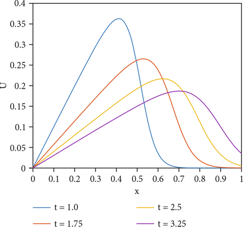
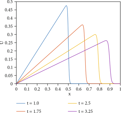
The numerical results for ε = 0.001, N = 30, and Δt = 0.025 are tabulated in Table 1, while those for ε = 0.0002, N = 30, and Δt = 0.025 are given in Table 2. These tables also include the total CPU time required for all calculations with absolute and relative errors. Based on the tables provided, the results obtained are relatively close to the exact results. It is noteworthy that the errors in our results decrease as the number of points used in time discretization increases. As time progresses, the absolute and relative errors in the tables gradually increase. However, the errors obtained in all schemes are small and acceptable for the viscosity values used in this problem.

Table 1. Solutions of Example 1 for [a, b] = [0, 1], ε = 0.001, Δt = 0.025, and N = 30 at different times.

T	T = 1.7 (m = 68)				T = 2.5 (m = 100)				T = 3.25 (m = 130)
x	TDFEM2	TDFEM3	TDFEM4	Exact	TDFEM2	TDFEM3	TDFEM4	Exact	TDFEM2	TDFEM3	TDFEM4	Exact
0.1	0.0588	0.0588	0.0588	0.0588	0.0400	0.0400	0.0400	0.0400	0.0317	0.0310	0.0308	0.0308
0.3	0.1765	0.1765	0.1765	0.1765	0.1200	0.1200	0.1200	0.1200	0.0928	0.0924	0.0923	0.0923
0.5	0.2971	0.2971	0.2941	0.2941	0.2000	0.2000	0.2000	0.2000	0.1545	0.1540	0.1539	0.1539
0.7	0.2800	0.2800	0.2800	0.2800	0.2800	0.2800	0.2800	0.2800	0.2155	0.2155	0.2154	0.2154
0.9	0.0000	0.0000	0.0000	0.0000	0.0000	0.0000	0.0000	0.0000	0.1115	0.1113	0.1113	0.1113
L_∞	8.4e − 07	6.2e − 07	3.1e − 07	—	6.3e − 05	3.5e − 05	2.2e − 05	—	9.6e − 04	2.1e − 04	1.2e − 05	—
	1.4e − 05	1.0e − 05	5.3e − 06	—	2.2e − 04	1.2e − 04	7.8e − 05	—	6.2e − 03	1.3e − 03	4.9e − 05	—
CPU (s)	0.20613	0.12145	0.09231	—	0.32181	0.19442	0.10135	—	0.96372	0.68208	0.23647	—

Table 2. Solutions of Example 1 for [a, b] = [0, 1], ε = 0.0002, Δt = 0.025, and N = 30 at different times.

T	T = 3.5 (m = 140)				T = 5 (m = 200)				T = 12 (m = 480)
x	TDFEM2	TDFEM3	TDFEM4	Exact	TDFEM2	TDFEM3	TDFEM4	Exact	TDFEM2	TDFEM3	TDFEM4	Exact
0.1	0.0285	0.0286	0.0286	0.0286	0.0200	0.0200	0.0200	0.0200	0.0081	0.0083	0.0083	0.0083
0.3	0.0856	0.0857	0.0857	0.0857	0.0600	0.0600	0.0600	0.0600	0.0252	0.0250	0.0250	0.0250
0.5	0.1428	0.1429	0.1429	0.1429	0.9998	0.1000	0.1000	0.1000	0.0418	0.0417	0.0417	0.0417
0.7	0.1999	0.2000	0.2000	0.2000	0.1399	0.1400	0.1400	0.1400	0.0580	0.0583	0.0583	0.0583
0.9	0.2572	0.2571	0.2571	0.2571	0.1798	0.1800	0.1800	0.1800	0.0749	0.0750	0.0750	0.0750
L_∞	8.2e − 05	5.9e − 05	2.8e − 05	—	2.3e − 04	8.8e − 05	5.2e − 05	—	2.1e − 04	9.6e − 05	2.4e − 05
	3.2e − 04	2.3e − 04	1.2e − 04	—	1.3e − 03	4.9e − 04	2.9e − 04	—	2.8e − 03	1.3e − 04	3.2e − 04
CPU (s)	0.42438	0.25004	0.19015	—	0.66255	0.40027	0.20866	—	1.98713	1.40428	0.68685

Tables 3 and 4 provide a comparison of numerical solutions obtained using cubic B-spline [14] and Hermite formula [17] based collocation methods at different time stages. The results demonstrate that our proposed methods based on FEM are more accurate, as the computed errors are smaller than the corresponding errors obtained by [14, 17]. Additionally, our proposed methods are more efficient in terms of time consumption, and thus, they are a better choice for solving problems of Burgers’ type.

Table 3. The comparison of error norms for at different times for [a, b] = [0, 1], ε = 0.005, N = 200, and Δt = 0.01 for Example 1.

	L_∞	CPU (s)	L_∞	CPU (s)	L_∞	CPU (s)
	T = 1.7		T = 2.5		T = 3.25
[14]	3.1153e − 04	—	1.8902e − 04	—	8.9839e − 03	—
[17]	7.5869e − 05	2.32813	1.1491e − 04	5.46875	7.9982e − 03	8.04688
TDFEM2	5.2134e − 05	2.32656	7.3965e − 05	3.68521	6.6734e − 04	5.82314
TDFEM3	3.3720e − 06	1.91070	3.8625e − 06	1.97382	4.0123e − 06	2.98236
TDFEM4	1.2123e − 07	1.00205	1.6543e − 07	1.68234	1.7238e − 07	2.01012

Table 4. The comparison of error norms for at different times for [a, b] = [0, 1], ε = 0.0005, N = 200, and Δt = 0.01 for Example 1.

	L_∞	CPU (s)	L_∞	CPU (s)	L_∞	CPU (s)
	T = 1.7		T = 2.5		T = 3.25
[14]	2.7577e − 02	—	2.5152e − 02	—	2.1049e − 02	—
[17]	1.5553e − 02	2.82813	4.5958e − 03	4.79688	2.3305e − 03	7.79688
TDFEM2	9.8156e − 05	2.82623	7.8888e − 05	3.86127	6.8023e − 04	4.23147
TDFEM3	4.2073e − 06	2.58453	4.1817e − 06	2.73270	4.3641e − 06	3.00005
TDFEM4	1.3218e − 07	1.01472	1.9234e − 07	1.80032	1.8724 − 07	2.225145

We examined the effect of increasing the number of finite elements and m values on the error norms, which are presented in Tables 5 and 6, respectively. It is observed that an increase in the number of finite elements leads to a significant reduction in the absolute error rate, as shown in Table 5. Moreover, as the value of m increases, the time step decreases, and the numerical solutions converge more closely to the exact solutions. The paper’s tables indicate that TDFEM4 is more accurate and economical than TDFEM2 and TDFEM3, requiring less computational cost and storage space.

Table 5. The error norms for Example 1 at different times for [a, b] = [0, 1], ε = 0.002, and Δt = 0.05(m = 40) at T = 2.

	N = 30	N = 40	N = 50	N = 30	N = 40	N = 50
	L_∞			CPU (s)
TDFEM2	5.8437e − 05	6.0234e − 06	5.8551e − 07	0.15200	0.24143	0.31245
TDFEM3	9.7731e − 06	7.1238e − 07	4.3719e − 08	0.02202	0.05324	0.10567
TDFEM4	4.0083e − 07	2.7283e − 08	2.7585e − 10	0.01001	0.03214	0.08273

Table 6. Comparison of the numerical solutions for Example 1 obtained with various values of m for [a, b] = [0, 1] and ε = 0.01 at T = 1 with the exact solutions.

x	m = 10			m = 40			m = 80			Exact
x	TDFEM2	TDFEM3	TDFEM4	TDFEM2	TDFEM3	TDFEM4	TDFEM2	TDFEM3	TDFEM4	Exact
0.1	0.099742	0.099747	0.099748	0.099745	0.099751	0.099752	0.099750	0.099752	0.099752	0.099752
0.3	0.294610	0.294608	0.294605	0.294607	0.294603	0.294604	0.294601	0.294604	0.294604	0.294604
0.5	0.250010	0.250008	0.250004	0.250006	0.250000	0.250000	0.250001	0.250000	0.250000	0.250000
0.7	0.001721	0.001725	0.001728	0.001728	0.001730	0.001731	0.001729	0.001731	0.001731	0.001731
0.9	0.000000	0.000000	0.000000	0.000000	0.000000	0.000000	0.000000	0.000000	0.000000	0.000000

Example 2. We consider Burgers’ equation with the initial condition,

(27)

and the boundary conditions,

(28)

and the following forcing term,

(29)

With the above conditions, the exact solution of the model equation is

(30)

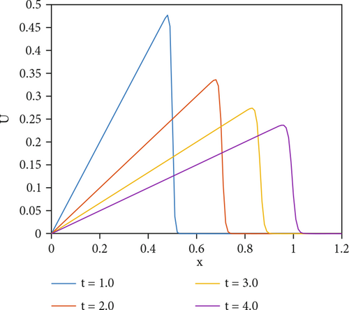
Figures 3 and 4 depict the physical behavior of the problem for ε = 0.0001 at T = 2 and ε = 0.00005 at T = 12 with N = 110 and Δt = 0.025, respectively. For the viscosity value of ε = 0.00005, the program took 4.358682 seconds to run, and a sharp descent is observed at 11.4 seconds. It is seen that the proposed method efficiently captures the shocks in the numerical solution.

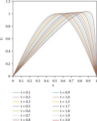
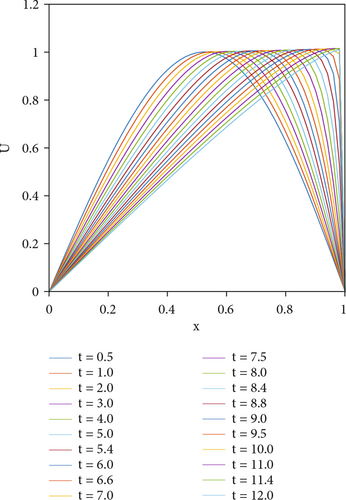
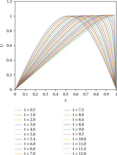
The accuracy of the presented methods is examined by computing the absolute and relative errors for smaller values of viscosity. In the present, the selection of viscosity value affects the errors in the proposed schemes. With decreasing viscosity values, the algorithm needs more finite elements to compute properly. As expected, the error norms are reduced by increasing the number of finite elements and decreasing the time step.

The absolute and relative errors for ε = 0.001, N = 30, and Δt = 0.01 and ε = 0.0001, N = 50, and Δt = 0.001 at different times are tabulated in Tables 7 and 8, respectively. These tables also provide the total CPU time required for all computations. It is seen from Tables 7 and 8 that the errors obtained in all schemes are quite small and acceptable for values of viscosity used in this problem. Our proposed numerical methods perform efficiently for small values of ε in a short computation time.

Table 7. L_∞ and

errors for Example 2 for ε = 0.001, N = 30, and Δt = 0.01.

x	TDFEM2				TDFEM3				TDFEM4
x	T = 0.1	T = 0.2	T = 1	T = 3.0	T = 0.1	T = 0.2	T = 1.0	T = 3.0	T = 0.1	T = 0.2	T = 1	T = 3
L_∞	1.24e − 04	3.39e − 05	8.22e − 06	3.84e − 06	2.22e − 05	2.15e − 05	1.35e − 06	4.77e − 07	1.52e − 05	1.35e − 05	1.59e − 06	2.01e − 07
	2.22e − 02	3.44e − 04	8.15e − 05	2.10e − 05	2.79e − 03	2.72e − 04	1.44e − 05	5.76e − 06	1.75e − 05	1.43e − 05	1.88e − 06	3.26e − 07
CPU	0.00470	0.00651	0.09213	0.69403	0.001029	0.00214	0.42312	0.15841	0.00024	0.00098	0.01478	0.10992

Table 8. L_∞ and

errors for Example 2 for ε = 0.0001, N = 50, and Δt = 0.001.

x	TDFEM2				TDFEM3				TDFEM4
x	T = 0.1	T = 0.2	T = 1	T = 3.0	T = 0.1	T = 0.2	T = 1.0	T = 3.0	T = 0.1	T = 0.2	T = 1	T = 3
L_∞	4.25e − 05	3.27e − 05	8.08e − 06	2.19e − 06	1.34e − 05	6.74e − 06	3.81e − 07	3.20e − 07	7.13e − 06	4.55e − 06	3.00e − 07	1.40e − 07
	2.25e − 03	1.32e − 04	4.83e − 05	9.44e − 06	1.69e − 04	7.47e − 05	6.35e − 07	3.38e − 07	9.43e − 06	7.54e − 06	5.58e − 07	2.00e − 07
CPU	0.56342	0.72103	1.25694	1.54123	0.32314	0.45426	0.86314	0.94213	0.20789	0.25456	0.73476	0.86738

In particular, the TDFEM4 can progress up to 12 seconds with less computational complexity and capture shocks at 11.4 seconds. Yet, the computed results of the method that used more points in discretization in time are more accurate in comparison with the other two combined methods and are free of choice of viscosity parameter. It can be inferred that the presented numerical methods are in quite good agreement with the exact solution and represent the physical properties of Burgers’ equation with forcing term accurately.

Example 3 (see [26].)Consider the model equation

(31)

with the initial condition,

(32)

and with the time-dependent nonhomogeneous boundary conditions,

(33)

Its exact solution is

(34)

In this example, the numerical results have been computed for the parameter values in Table 9. The accuracy of the three combined methods has been demonstrated based on the error norms, and the presented schemes have been compared with each other in terms of their advantages and disadvantages. It is seen that the combined methods have more accurate results even with the use of fewer finite elements than some studies in the literature, and the comparisons have shown that the present schemes offer better results than the numerical schemes given in [26]. This problem was studied in [18], yet there are no numerical results to compare with our results. Therefore, we do not have elaborate details.

Table 9. Numerical results of Example 3 for ε = 0.0001, N = 50, and Δt = 0.001 at T = 1.

x	TDFEM2	TDFEM3	TDFEM4	Exact
0.5	0.00075331	0.00075330	0.00075330	0.00075330
0.7	0.00106213	0.00106212	0.00106211	0.00106211
0.9	0.00137922	0.00137919	0.00137919	0.00137919
1.1	0.00170819	0.00170818	0.00170818	0.00170818
1.3	0.00205407	0.00205406	0.00205405	0.00205405
1.5	0.00242397	0.00242396	0.00242396	0.00242396
L_∞	2.013e − 08	1.254e − 08	9.874e − 09	—
	2.655e − 05	1.103e − 06	1.088e − 08	—
CPU (s)	0.20614	0.12123	0.07564

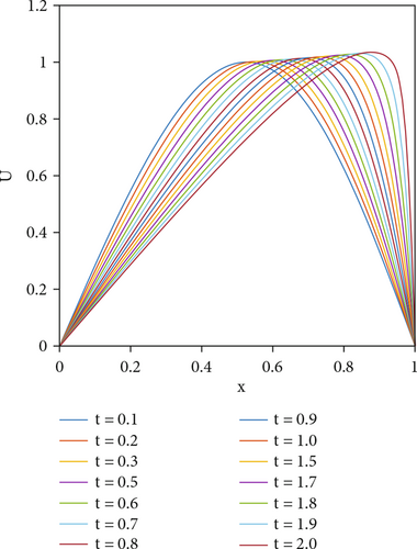
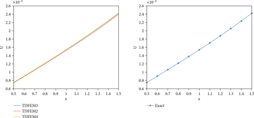
Figure 5 displays the physical behavior of the solution function at T = 2, for ε = 0.001, N = 40, and Δt = 0.01. The numerical results agree with the exact results, indicating that the three combined methods used in this study are accurate, especially the method that used more points in discretization in time which was found to be more accurate than the other two methods. We can conclude that these combined methods are more accurate than some other existing methods in the literature.

4. Conclusions and Recommendations

In the present work, the three combined methods based on the backward finite difference and Galerkin finite element schemes have been introduced and applied for solutions of the Burgers’ equation with forcing term accurately. To demonstrate the efficiency of the proposed newly combined methods, three test examples are included and the numerical computations are performed for various values of the parameters. The computed results have revealed that the proposed methods are computationally powerful, highly accurate, and capable of solving the model equation. The numerical results are seen to be relatively more accurate than some of the existing results in the literature. The methods are also quite convenient to generate computer codes in any programming language. As well, the presented methods in this article seem to be a very robust alternative to solve the problem by preserving the physical properties of the Burgers’ equation. Based on the currently proposed methods, further studies can focus on solving the Burgers’ type equations as well as other PDEs arising in various fields of science and engineering.

Disclosure

The authors declare that they have not used artificial intelligence (AI) tools in the preparation of this article.

Conflicts of Interest

The authors did not report any potential conflicts of interest.

Acknowledgments

The authors would like to thank Dr Murat Sari (Istanbul Technical University) for his valuable comments on this paper. The first author would like to thank the Science Fellowships and Grant Programs Department of TUBITAK (TUBITAK BIDEB) for supporting her academic research.

Open Research

Data Availability

Data will be made available on request.

References

1 Bateman H., Some recent researches on the motion of fluids, Monthly Weather Review. (1915) 43, no. 4, 163–170, https://doi.org/10.1175/1520-0493(1915)43<163:SRROTM>2.0.CO;2.
10.1175/1520-0493(1915)43<163:SRROTM>2.0.CO;2
Google Scholar
2 Burgers J. M., Mathematical examples illustrating relations occurring in the theory of turbulent fluid motion, In Selected Papers of JM Burgers, 1995, Springer Netherlands, Dordrecht, 281–334, https://doi.org/10.1007/978-94-011-0195-0_10.
10.1007/978-94-011-0195-0_10
Google Scholar
3 Burgers J. M., A mathematical model illustrating the theory of turbulence, Advances in Applied Mechanics. (1948) 1, 171–199, https://doi.org/10.1016/S0065-2156(08)70100-5, 2-s2.0-77956834067.
10.1016/S0065-2156(08)70100-5
Google Scholar
4 Hopf E., The partial differential equation 𝑢𝑡 + 𝑢𝑢𝑥 = 𝜇𝑢𝑥, Communications on Pure and Applied Mathematics. (1950) 3, no. 3, 201–230, https://doi.org/10.1002/cpa.3160030302, 2-s2.0-84980078224.
10.1002/cpa.3160030302
Web of Science® Google Scholar
5 Cole J. D., On a quasi-linear parabolic equation occurring in aerodynamics, Quarterly of Applied Mathematics. (1951) 9, no. 3, 225–236, https://doi.org/10.1090/qam/42889.
10.1090/qam/42889
Web of Science® Google Scholar
6 Sinuvasan R., Tamizhmai K., and Leach P., Algebraic resolution of the Burgers’ equation with forcing term, Pramana. (2017) 88, 1–6, https://doi.org/10.1007/s12043-017-1382-3, 2-s2.0-85019258569.
10.1007/s12043-017-1382-3
Web of Science® Google Scholar
7 Kadalbajoo M. K., Sharma K. K., and Awasthi A., A parameter-uniform implicit difference scheme for solving time-dependent Burgers’ equation, Applied Mathematics and Computation. (2005) 170, 1365–1393, https://doi.org/10.1016/j.amc.2005.01.032, 2-s2.0-27144488332.
10.1016/j.amc.2005.01.032
Web of Science® Google Scholar
8 Zeytinoglu A., Sari M., and Pasaoglu B. A., Numerical simulations of shock wave propagating by a hybrid approximation based on high-order finite difference schemes, Acta Physica Polonica A. (2018) 133, 140–151, https://doi.org/10.12693/aphyspola.133.140, 2-s2.0-85042268861.
10.12693/APhysPolA.133.140
CAS Web of Science® Google Scholar
9 Kumar R. and Chandrashekar P., Efficient seventh order WENO schemes of adaptive order for hyperbolic conservation laws, Computer and Fluids. (2019) 190, 49–76, https://doi.org/10.1016/j.compfluid.2019.06.003, 2-s2.0-85067001773.
10.1016/j.compfluid.2019.06.003
Web of Science® Google Scholar
10 Mukundan V. and Awasthi A., Efficient numerical techniques for Burgers’ equation, Applied Mathematics and Computation. (2015) 262, 282–297, https://doi.org/10.1016/j.amc.2015.03.122, 2-s2.0-84929104818.
10.1016/j.amc.2015.03.122
Web of Science® Google Scholar
11 Aksan E. N., A numerical solution of Burgers’ equation by finite element method constructed on the method of discretization in time, Applied Mathematics and Computation. (2005) 170, no. 2, 895–904, https://doi.org/10.1016/j.amc.2004.12.027, 2-s2.0-27144517638.
10.1016/j.amc.2004.12.027
Web of Science® Google Scholar
12 Ozis T., Aksan E. N., and Ozdes A., A finite element approach for solution of Burgers’ equation, Applied Mathematics and Computation. (2003) 139, no. 2-3, 417–428, https://doi.org/10.1016/S0096-3003(02)00204-7, 2-s2.0-0037448173.
10.1016/S0096-3003(02)00204-7
Web of Science® Google Scholar
13 Chen Y. and Zhang T., A weak Galerkin finite element method for Burgers’ equation, Journal of Computational and Applied Mathematics. (2019) 348, 103–119, https://doi.org/10.1016/j.cam.2018.08.044, 2-s2.0-85053079669.
10.1016/j.cam.2018.08.044
Web of Science® Google Scholar
14 Dag I., Irk D., and Sahin A., B-spline collocation methods for numerical solutions of the Burgers′ equation, Mathematical Problems in Engineering. (2005) 2005, 18, https://doi.org/10.1155/MPE.2005.521, 2-s2.0-31044432795, 928423.
10.1155/MPE.2005.521
Google Scholar
15 Mittal R. C. and Jain R. K., Numerical solutions of nonlinear Burgers’ equation with modified cubic B-splines collocation method, Applied Mathematics and Computation. (2012) 218, no. 15, 7839–7855, https://doi.org/10.1016/j.amc.2012.01.059, 2-s2.0-84858333742.
10.1016/j.amc.2012.01.059
Web of Science® Google Scholar
16 Soliman A. A., A Galerkin solution for Burgers′ equation using cubic B-spline finite elements, Abstract and Applied Analysis. (2012) 2012, 15, https://doi.org/10.1155/2012/527467, 2-s2.0-84874927390, 527467.
10.1155/2012/527467
Google Scholar
17 Abdullah M., Yaseen M., and Sen M. D. L., An efficient collocation method based on Hermite formula and cubic B-splines for numerical solution of the Burgers’ equation, Mathematics and Computers in Simulation. (2022) 197, 166–184, https://doi.org/10.1016/j.matcom.2022.02.013.
10.1016/j.matcom.2022.02.013
Web of Science® Google Scholar
18 Sari M., Tunc H., and Seydaoglu M., Higher order splitting approaches in analysis of the Burgers’ equation, Kuwait Journal of Science. (2019) 46, no. 1.
Web of Science® Google Scholar
19 Gulen S., An efficient hybrid method based on cubic B-spline and fourth-order compact finite difference for solving nonlinear advection–diffusion–reaction equations, Journal of Engineering Mathematics. (2023) 138, no. 1, https://doi.org/10.1007/s10665-022-10249-0.
10.1007/s10665-022-10249-0
PubMed Web of Science® Google Scholar
20 Arora G., Mishra S., Emaifar H., and Khademi M., Numerical simulation and dynamics of Burgers’ equation using the modified cubic B-spline differential quadrature method, Discrete Dynamics in Nature and Society. (2023) 2023, 8, https://doi.org/10.1155/2023/5102374, 5102374.
10.1155/2023/5102374
Web of Science® Google Scholar
21 Khan M. I., Rauf A., and Shah A., Numerical investigation of viscous effects on the nonlinear Burgers’ equation, Turkish Journal of Mathematics. (2021) 45, no. 1, 529–539, https://doi.org/10.3906/mat-2001-7.
10.3906/mat-2001-7
Web of Science® Google Scholar
22 Soheili A. R., Arabameri M., and Barfeie M., RBFs meshless method of lines based on adaptive nodes of Burgers’ equations, Iranian Journal of Numerical Analysis and Optimization. (2015) 5, no. 1, 49–61, https://doi.org/10.22067/IJNAO.V5I1.32882.
10.22067/IJNAO.V5I1.32882
Google Scholar
23 Namjoo M., Zeinadini M., and Zibaei S., Nonstandard finite-difference scheme to approximate the generalized Burgers–Fisher equation, Mathematicsl Methods in the Applied Sciences. (2018) 41, no. 17, 8212–8228, https://doi.org/10.1002/mma.5283, 2-s2.0-85062638072.
10.1002/mma.5283
Web of Science® Google Scholar
24 Kaur R., Shallu V., Kukreja K., and Parumasur N., Two different temporal domain integration schemes combined with compact finite difference method to solve modified Burgers’ equation, Ain Shams Engineering Journal. (2022) 13, no. 1, article 101507, https://doi.org/10.1016/j.asej.2021.05.021.
10.1016/j.asej.2021.05.021
Web of Science® Google Scholar
25 Reddy J. N., An Introduction to the Finite Element Method, 2006, 3rd edition, McGraw-Hill, Singapore.
Google Scholar
26 Iskandar L. and Mohsen A., Some numerical experiments on the splitting of Burgers equation, Numerical Methods for Partial Differential Equations. (1992) 8, no. 3, 267–276, https://doi.org/10.1002/num.1690080303, 2-s2.0-0026866334.
10.1002/num.1690080303
Google Scholar
27 Rektorys K., The Method of Discretization in Time and Partial Differential Equations, 1982, D. Reidel Publishing Company, Holland.
Google Scholar

All articles

A New Efficient Hybrid Method Based on FEM and FDM for Solving Burgers’ Equation with Forcing Term

Abstract

1. Introduction

2. Materials and Methods

2.1. Two-Point Discretization in Time and Galerkin Finite Element Method (TDFEM2)

2.2. Three-Point Discretization in Time and Galerkin Finite Element Method (TDFEM3)

2.3. Four-Point Discretization in Time and Galerkin Finite Element Method (TDFEM4)

3. Numerical Experiments

4. Conclusions and Recommendations

Disclosure

Conflicts of Interest

Acknowledgments

Open Research

Data Availability

References

Figures

References

Information

About Wiley Online Library

Help & Support

Opportunities

Connect with Wiley

A New Efficient Hybrid Method Based on FEM and FDM for Solving Burgers’ Equation with Forcing Term

Abstract

1. Introduction

2. Materials and Methods

2.1. Two-Point Discretization in Time and Galerkin Finite Element Method (TDFEM2)

2.2. Three-Point Discretization in Time and Galerkin Finite Element Method (TDFEM3)

2.3. Four-Point Discretization in Time and Galerkin Finite Element Method (TDFEM4)

3. Numerical Experiments

4. Conclusions and Recommendations

Disclosure

Conflicts of Interest

Acknowledgments

Open Research

Data Availability

References

Figures

References

Related

Information