One of the central concerns in ecology is assessing the impact of environmental changes, such as global temperature shifts, on the dynamic interactions between predators and prey across diverse ecosystems. This study explores the relationship between prey and predator populations in the context of climate-induced temperature changes. Utilizing linearization and the Lyapunov approach, we analyze the local and global stability of the system’s equilibrium points. Applying Sotomayor’s theorem, we further investigate the local bifurcation of the fixed points. Additionally, the persistence of the model system is studied. The ecological models developed in this research aim to explore the stability of these predator–prey systems and provide insights to prevent the decline of endangered species. Numerical simulations are conducted to study the impact of environmental changes on the proposed models. The simulation results indicate that the temperature dependence of the predator–prey population dynamics is directly proportional to the size of the reserved habitat area for the prey when the temperature is high. These findings suggest that the preservation of sufficient habitat reserves plays a crucial role in promoting the long-term survival of species and stabilizing their ecological interactions.

1. Introduction

One of the most essential components of biological activity is the biosphere, which is responsible for driving changes in the environment and ecology. Refuges play a crucial role in conservation management, as they have the potential to protect species from difficult-to-manage threats such as changing climate, extreme events (e.g., drought, fire), and biotic threats (e.g., disease, invasive species) [1]. According to Oxford University Press (2019), a “refugium” is a place where a population of organisms can endure challenging conditions without fear of hardship, danger, or being sought after [2]. Since prey escape has a major impact on the system’s dynamic behavior, it is an essential component of the prey–predator system. It is known that in many dynamic systems, prey react to a predator attack by seeking refuge, which allows them to escape from the predator.

The relationship between climate change and the distribution and abundance of various organisms has been the subject of much research; as a result of their incapacity to adapt to their changing environment, some species have declined or even gone extinct [3, 4]. One of the most popular methods for predicting future range boundaries is the climate envelope method, which estimates a species’ fundamental niche space by utilizing correlations between observed environmental variables and the species’ current range boundaries [5]. Nevertheless, recent studies have revealed that organism distribution predictions based on body temperature differ significantly from those based only on environmental factors [6]. Understanding how weather and climate affect body temperature is especially crucial when studying predator–prey interactions [7].

Through a variety of mechanisms, such as changing the quantity and quality of vegetation that primary consumers depend on for foraging, climate variation and climate change may affect predator–prey interactions. This could result in differentiating foraging strategies and patterns of space use [8]. Temperature variations in the climate may also have an effect on prey’s nutritional status, which could alter how they perceive the risk of predators and react to attacks [9]. Climate change may affect the interactions between all species in a community, but predators are more vulnerable to environmental disturbance than plant herbivores, which could have important ramifications for the structure and functioning of the community [10].

Many species have varying climates, which are brought on by variables including humidity, temperature, rainfall, food availability, shifts in daylight, and elements that impact population survival in ecological communities [11]. Temperature affects ecological communities through its effects on the physiological performance of individuals. Temperature variability in the biosphere is having an increasingly noticeable impact on biological systems. Because of this, an organism’s survival and reproduction directly decline when its equilibrium with its surroundings is disturbed, which has an impact on population distribution across different geographic areas. Indeed, problems with temperature, population dynamics, species stability forecasting, and understanding population dynamics when behavior shifts due to climate change all have an impact on prey–predator systems.

The dynamics of prey–predator systems with prey refuge have been extensively studied using mathematical models. Refuges can have stabilizing or destabilizing effects, impacting prey regulation and population outbreaks [12]. Mismanagement, overexploitation, overpredation, and climate change contribute to prey refuges, necessitating steps like designating reserved regions to protect populations [13, 14]. As mentioned in [15], climate variability (through drought) has the potential to throw organisms out of balance with their surroundings.

In this context, we address a gap in the existing literature by incorporating temperature variability and prey refugees. Our study is aimed at examining the local and global stability associated with equilibrium, providing insights into the dynamics of prey–predator systems under changing environmental conditions. Additionally, we note the ecological significance and look into predator–prey dynamics as well as how temperature variability affects the stability of the system. The dynamic result of the system is examined through numerical simulations carried out with MATLAB programming.

2. Mathematical Model Formulation

2.1. Model Assumptions

The effect of climate alteration on the prey–predator is intuitive. Considering this into account made the following assumptions. In this research, the food web consists of three species: P (the prey species in the unreserved area), N (the prey species in the reserved area), and R (the predator species at a specific location) and T (temperature due to climate change) at time t. Predator feeding behavior is governed by the Holling Type-II functional response, which is contingent upon favorable weather conditions and seasonal variations in the predator’s attack rate. Predation rates are temperature dependent. The maximum temperature where prey disturbance is high is T_max and the balanced temperature for prey is T₀, r₁(T) is the intrinsic growth rate (temperature dependent) of the prey species in the unreserved area, r₂(T) is the intrinsic growth rate (temperature dependent) of the prey species in the reserved area, μ(T) is the predation rate (temperature dependent), and prey refugees and natural death rate of predator populations are temperature independent (T). The conservation management (especially in light of temperature variability) identifies potential refugees’ location. When there is significant temperature fluctuation, the populations move around. Both the prey and the predator coexist in a free region. Prey populations can migrate from unreserved to reserved areas, but predator populations are not allowed to enter the reserved area, and vice versa is not permissible. The movement can be attributed to various factors such as drought, deforestation (potentially for the production of charcoal), and poor resource management. These issues have collectively contributed to the current situation.

We hypothesise that for prey species, the presence of an intraspecific competition factor results in a density-dependent death factor [16]. The fear of being eaten influences the way the prey give birth, and they hide in a variety of shelters that depend on their interaction with the predator populations. Incorporating these assumptions, the deterministic mathematical model equations have the form

(1)

with P(t₀) = P₀ ≥ 0, N(t₀) = N₀ ≥ 0, R(t₀) = R₀ ≥ 0, T(t₀) = T₀ ≥ 0, 0 < c < 1.

Because of the refuge’s limited resources or size, there would be a maximum amount of prey that the area could sustain. Table 1 discusses the parameters in the model system and their biological significance.

Table 1. Biological meaning of parameters in model system (1).

Variables and parameters	Biological meaning
P(t)	The population size of the prey in the unreserved area at time t.
N(t)	The population size of the prey in the reserved area at time t.
R(t)	The population size of the predator in the free region at time t.
T(t)	Temperature due to climate change at time t.
r₁(T)	Intrinsic growth rate (temperature dependent) of the prey species in the unreserved area
r₂(T)	Intrinsic growth rate (temperature dependent) of the prey species in the reserved area.
r₃	Increment rate of temperature.
μ(T)	Predation rate (temperature dependent).
α	Half-saturation constant.
c	Conversion efficiency at specific location.
β	Natural death rate of predator.
δ	The migration rate of the prey population from the unreserved area to the reserved area.
k₁, k₂	The carrying capacity of the prey in the unreserved and protected region, respectively.

Utilizing the parameters, the dimensionless of the model system (1), p = P/K₁, n = N/K₂, r = r₂(T)R/r₁(T)K₁, τ = r₁(T)t, T = T_maxq. The system (1)’s scaled version is reduced to the form

(2)

where η = δ/r₁(T), σ(q) = μK₁/αr₁(T), m = K₁/α, φ(q) = r₂(T)/r₁(T), γ = δK₁/K₂r₁(T), ξ(q) = cμK₁/αr₁(T), ϕ = β/r₁(T), β₁ = r₃(T)/r₁(T), α₁ = T₀/T_max.

According to the study [17, 18], the parameter assignments utilize the findings to specify the annual per capita growth rate of temperature T. The parameter assignments are made in such a way that

(3)

where T ∈ (T₀, T_m) is defined to be temperature measured in °C from a prescribed base temperature of °C (that is, T ≡ ^°C − 10^°C).

The predator’s deadly maximum temperature T ≡ 30⁰ or higher is the point at which the life process is irreversibly disrupted.

The rate at which prey migrates from unreserved to reserved areas, contingent upon predator density, is presumed to be positive and to escalate with the number of prey species, N. In principle, this implies that as the number of predators in the unreserved region increases, more prey either departs or collaborative hunting enhances the predators’ ability to capture prey populations and procure food.

3. Model Analysis

3.1. Positivity, Uniqueness, and Boundedness of Solution

The positivity, uniqueness, and boundedness of the solutions of the model system (2) are all examined in this section.

3.1.1. Positivity of the Solution

For a given initial condition (n(0), p(0), r(0), q(0)), we observe that the system (2) is well-posed. We show positivity of the solutions in the following proposition:

Proposition 1. The solution (p(τ), n(τ), r(τ), q(τ)) of the model system with a positive initial condition (p₀, n₀, r₀, q₀) is positive.

Proof 1. Here, it is possible to write the first equation of the model system (2) dp/dτ = p(1 − p) − ηp − σ(pr/(1 + mp)) as

( )

where h(τ) = (η + (σr/1 + mp) − 1). This is a Bernoulli-type differential equation.

Hence,

( )

Since p is positive, the second equation can be written in the form

( )

This implies

( )

Then

( )

For the third equation of system (2)

( )

Integration gives r(τ) = r₀e^{((ξp/1 + mp) − ϕ)τ} which is positive.

Finally, the fourth equation

( )

That is,

( )

Solving this equation, we obtain

( )

Hence, for positive initial conditions, all solutions of model system (2) are positive for all t ≥ 0.

3.1.2. Boundedness of Solutions of the Model System

The following proposition serves to establish the boundedness of the solution model system (2).

Proposition 2. All solutions (p(τ), n(τ), r(τ), q(τ)) of the model system (2) with nonnegative initial condition (p₀, n₀, r₀, q₀) is uniformly bounded in the region

( )

where

( )

Proof 2. We present the following sum relation function in order to demonstrate model system (2)’s boundedness, defined as the total population (2).

Differentiating Z(τ) with respect to τ

( )

Since dp/dτ = p(1 − p) − ηp − σ(q)(pr/(1 + mp)), dn/dτ = φ(q)n(1 − n) + γp, dr/dτ = ξ(q)(pr/(1 + mp)) − ϕr.

( )

Adding ϕZ on both sides for positive ϕ, we have

( )

Therefore, Z(τ) = (ϕ + φ(ϕ + 2)/ϕφ) + ce^−ϕτ, where c is constant.

As τ⟶∞, Z⟶(ϕ + φ(ϕ + 2)/ϕφ), that is 0 < Z(τ) ≤ (ϕ + φ(ϕ + 2)/ϕφ) which is bounded. It follows each of the state variables p(τ), n(τ), r(τ) that are also bound.

To show the boundedness of q(τ), we consider the last equation of the model system.

( )

After simplification, we obtain

( )

Hence, as τ⟶∞, q⟶β₁ + α₁, that is 0 < q(τ) ≤ (β₁ + α₁) which is bounded.

Here, one can conclude that all the solutions of the system (2) that are initiated in are attracted to the region

( )

Therefore, the solutions p(τ), n(τ), r(τ) and q(τ) are bounded and positive invariant under the given condition.

3.1.3. Uniqueness

The solution of a system starting in the nonnegative octant is bounded, and the right side of the model system (2) is continuous and has continuous partial derivatives of all orders in a domain Ω of the positive octant . Therefore, the solution of the model system (2) with nonnegative initial condition exists and is unique.

3.2. Existence of Equilibrium Points

We demonstrate the existence of a positive solution of model system (2) with omitting equation of temperature in this section. Because it can be difficult to comprehend how temperature and threshold vital rates relate to one another.

The equilibrium points of the model system (2) are solutions of a nonlinear system equation.

( )

After solving the above system, we find the following equilibrium points:

i.
The equilibrium points E₀ = (0, 0, 0) and E₁ = (0, 1, 0) exist with no condition.
ii.
There are also additional equilibrium points. The third equilibrium point is , and it exists if 0 < η < 1.

The interior equilibrium is E_3,4 = (p^∗, n^∗, r^∗), where

( )

The interior equilibrium points exist if ξ > mϕ, and 0 < (ϕ/(ξ − mϕ)) + η < 1.

3.3. Local Stability of the Equilibrium Point

Utilizing the eigenvalue method, we examine the local dynamic behavior of the model system (2) around each of the equilibrium points shown above.

The stability of an equilibrium point is found by looking at the sign of the matrix’s eigenvalues [19, 20]. The Jacobian matrix of the model system (2) looks as

(4)

We examine local stability and the equilibria of system (2) in the following propositions.

Proposition 3. The trivial equilibrium point E₀(0, 0, 0) is unstable.

Proof 3. The Jacobian matrix of the model (2) at E₀ is

(5)

Then, clearly, the eigenvalues of J(0, 0, 0) are λ₁ = 1 − η, λ₂ = φ, λ₃ = −ϕ.

Hence, the trivial equilibrium point E₀ is saddle point which is unstable. This biologically means that total annihilation is not possible.

Proposition 4. The equilibrium point E₁(0, 1, 0) is locally asymptotically stable if η > 1.

Proof 4. The Jacobian matrix at E₁ takes the form

( )

The three eigenvalues of the Jacobian matrix are λ₁ = 1 − η, λ₂ = −φ, and λ₃ = −ϕ.

Therefore, E₁ is locally asymptotically stable, if η > 1.

This, in turn, biologically means that prey populations in the unreserved area survive.

Proposition 5. The predator-free equilibrium point E₂(p^∗, n^∗, 0) is locally asymptotically stable if either of the following is true:

( )

Proof 5. The Jacobian matrix of the model system (2) at E₂ is

(6)

The eigenvalues of the Jacobian matrix J(p^∗, n^∗, 0) are and λ₃ = (−(mϕ − ξ)(ϕ − (1 − η)))/(m(1 − η) + 1).

Here, we notice that since 0 < η < 1, λ₁ and λ₂ are negative. Moreover, the third eigenvalue λ₃ < 0 if ξ − ϕm < 0 and ϕ − (1 − η) > 0, or ξ − ϕm > 0 and ϕ − (1 − η) < 0.

Proposition 6. The positive equilibrium point E₃(p^∗, n^∗, r^∗) is locally asymptotically stable in , if

(7)

where the expressions of A₁, A₂, and A₃ are as presented below.

Proof 6. The Jacobian matrix of the system (2) at the positive equilibrium point E₃(p^∗, n^∗, r^∗) can be written as

(8)

The eigenvalues are obtained from the characteristic equation Det(J(E₃) − λI) = 0 and can be written as

( )

Accordingly, the characteristic equation Det(J(E₃) − λI) = 0 is

( )

Here,

( )

Hence, by Routh–Hurwitz criteria, the interior equilibrium point is locally asymptotically stable under the conditions A₁ > 0, A₂ > 0, A₁A₂ − A₃ > 0, combined with ξ > mϕ, 0 < (ϕ/(ξ − mϕ)) + η < 1.

Proposition 7. The interior equilibrium point E₄(p^∗, n^∗, r^∗) is locally asymptotically stable in the positive orthant if the following conditions are met:

( )

where the expressions for B₁, B₂, and B₃ are as given below.

Proof 7. The Jacobian matrix of the model system at the equilibrium point E₄(p^∗, n^∗, r^∗) becomes

(9)

where

( )

and exists if ξ > mϕ, and 0 < (ϕ/(ξ − mϕ)) + η < 1.

The eigenvalues are obtained from the characteristic equation Det(J(E₃) − λI) = 0 and can be written as

( )

where

( )

The characteristic equation Det(J(E₃) − λI) = 0 becomes

( )

where

( )

Here, the explicit expressions are

( )

where

, and

( )

Hence, we can conclude by the Routh–Hurwitz criteria that the interior equilibrium point E₄ is locally asymptotically stable if the conditions B₁ > 0, B₂ > 0, B₁B₂ − B₃ > 0, along with ξ > mϕ, 0 < (ϕ/(ξ − mϕ)) + η < 1, are satisfied.

3.4. Global Stability

The Lyapunov function is a powerful tool for figuring out the global stability of an equilibrium point [21–24].

Theorem 1. The steady state E₂(p^∗, n^∗, 0) is globally asymptotically stable in the region R₊ = {(p, n): p > 0, n > 0} if it exists and is locally asymptotically stable in the interior of the region

Proof 8. Let E₂(p^∗, n^∗, 0) be locally asymptotically stable in the region R₁. The model system (2) can be reduced to the form

( )

Consider the function

( )

It is Dulac’s in the region R₊ and .

Then, and

( )

Thus, the system has no periodic orbit in pn-plane region, and hence, E₂(p^∗, n^∗, 0) is globally asymptotically stable in the region R₊ = {(p, n): p > 0, n > 0}.

Theorem 2. The equilibrium point E₃(p^∗, n^∗, r^∗) is globally asymptotically stable.

Proof 9. We consider a Lyapunov function of the form

( )

where C₁ and C₂ are positive constants to be determined. Differentiating the function V with respect to time τ,

( )

and substituting in the expressions for dp/dτ, dn/dτ, dr/dτ from the scaled equation of the model system and taking under consideration (p^∗, n^∗, r^∗) that is the equilibrium point, we have

( )

Rearranging it becomes

( )

Compactly, this can be expressed as

( )

Choosing C₁ = 1, C₂ = r^∗ψ_p(p^∗)/p^∗ψ_r(r^∗), we have

( )

Since the terms 1 + (p^∗ + η − 1)/p and 1 + ((n^∗ − 1)/n) are positive, then (dV/dτ) ≤ 0, and V(τ) is a Lyapunov function. Hence, the positive equilibrium point E₃(p^∗, n^∗, r^∗) of the model system (2) is globally asymptotically stable.

3.5. Persistence

A system is considered persistent if none of its states approach zero, signifying that no species within the biological system face extinction. A system is said to be persistent if one of its states never approaches zero, meaning that no member of species that comprises the biological system could go extinct. As depicted, the equilibrium point E₀(0, 0, 0) is unstable in the p and n-directions but asymptotically stable in the r-direction. Equilibrium point E₁(0, 1, 0) lies along the positive n-axis and is asymptotically stable in the n and r-directions, yet unstable in the p-direction when 0 < η < 1. There exists no equilibrium point on the p and r-axis. Along with the presumptions mentioned above, the following is true.

1.
The right-hand side of the model system (2) is C¹ in (p, n, r).
2.
All solutions of the system (2) with initial conditions are bounded in forward time according to Proposition 2.
3.
E₁(0, 1, 0) exists and hyperbolic saddle point if 0 < η < 1.
4.
An equilibrium point E₂(p^∗, n^∗, 0) in the pn-plane exists, and it is unstable in the positive direction orthogonal to the pn-plane if ξ − mϕ > 0 and ϕ − (1 − η) > 0 or ξ − mϕ < 0 and ϕ − (1 − η) < 0. Since E₂(p^∗, n^∗, 0) is locally asymptotically stable whenever it exists, it is globally asymptotically stable with no limit cycles around this point [25]. In the pn-plane, the stable point is designated as the unique equilibrium point E₂. This theorem generalized the existence of the model system (2). The proof of positivity and boundedness is also provided in Proposition 1 and Proposition 2.

The observations outlined above are formalized into the following theorem.

Theorem 3. The model system (2) meets the necessary conditions for persistence whenever the equilibrium point E₂(p^∗, n^∗, 0) exists, provided that 0 < η < 1, ξ − mϕ < 0 and ϕ − (1 − η) < 0, or ξ − mϕ > 0 and ϕ − (1 − η) > 0.

Proof 10. Suppose Φ(Y) be the orbit through the point in the positive octant Y = (p, n, r) with p > 0, n > 0, r > 0. Let ρ(Y) be the ω-limit set of Φ(Y). Note that ρ(Y) is bounded.

We claim that E₀ does not belong to ρ(Y). If E₀ ∈ ρ(Y), then by Lemma A₁ of [25], there exists another point u in ρ(Y) ⋂ W^s(E₀) where W^s(E₀) denote the stable manifold of E₀. Since, Φ(u) and W^s(E₀) in the r-direction, we conclude that Φ(u) is unbounded, which is a contradiction.

Similarly, E₁ ∉ ρ(Y). If E₁ ∈ ρ(Y), then there exists a point u in ρ(Y) ⋂ W^s(E₁) where W^s(E₁) denote the stable manifold of E₁. Since, Φ(u) lies ρ(Y) and W^s(E₁) in the nr-direction, we conclude that Φ(u) is unbounded, which is a contradiction.

In the same way, E₂ ∉ ρ(Y). If E₂ ∈ ρ(Y), the condition 0 < η < 1, ξ − mϕ > 0 and ϕ − (1 − η) > 0 or ξ − mϕ < 0 and ϕ − (1 − η) < 0 implies that E₂ is a stable point and W^s(E₂) is the pnr-direction; again, we conclude that unbounded orbit lies in ρ(Y), which is a contradiction.

As a result, the model system (2) persists and ρ(Y) lies in the positive octant. Ultimately, the model system (2) is dissipative and only the closed orbits and equilibria form the ω-limit set of the solutions in the boundary of .

3.6. Local Bifurcation Analysis

Many ecologists are exploring the applications of mathematics in species biology.

Theorem 4. The model system (2) undergoes no bifurcation around the trivial equilibrium point E₀(0, 0, 0).

Proof 11. The Jacobian matrix around the equilibrium point E₀(0, 0, 0) is

( )

Computing the characteristic equation, we have λ₁ = 1 − η, λ₂ = φ, λ₃ = −ϕ; hence, it is a saddle node. If 1 − η = 0, then there is a characteristic root with eigenvalue λ = 0 and eigenvectors corresponding to the matrix J and J^T given as

( )

respectively. Take η as a parameter to denote the solution of 1 − η = 0 as η = η^∗. The derivative of the model system (2) with respect to parameter η is

( )

Further

( )

and hence f_η(E₀, η = η^∗) = (0, 0, 0)^T.

On the other hand

( )

and

( )

Computing the third condition of Sotomayor’s theorem w^T[D²f(E₀, η = η^∗)(V, V)], using the following:

(10)

Thus,

( )

Then, we investigate the condition: w^Tf_η(E₀, η = η^∗) = 0, w^T[Df_η(E₀, η = η^∗)V] = 0, w^T[D²f(E₀, η = η^∗)(V, V)] = 0.

Thus, there is no bifurcation around the trivial fixed point E₀(0, 0, 0), which is unstable.

Theorem 5. The model system (2) exhibits a transcritical bifurcation at η = 1 near the steady state E₁.

Proof 12. The Jacobian matrix at E₁ takes the form

( )

The three eigenvalues of the Jacobian matrix are λ₁ = 1 − η, λ₂ = −φ, and λ₃ = −ϕ, which is stable if η > 1. By substituting E₁(0, 1, 0) with η = 1 in the Jacobian matrix J(E₁), the characteristic equation has zero eigenvalues.

The eigenvectors V and w which are associated to zero eigenvalues of matrices J and J^T, respectively, are

( )

Let f be the right-hand side of the model system (2),

(11)

The derivative of the model system (2) with respect to the control parameter η is

( )

It follows that

( )

Hence, f_η(E₁, η) = (0, 0, 0)^T.

The first condition of Sotomayor’s theorem is satisfied:

( )

In addition,

( )

The second condition of Sotomayor’s theorem is again satisfied:

( )

Computing the third condition of Sotomayor’s theorem w^T[D²f(E₁, η)(V, V)], using Equation (10), we obtain

( )

where

( )

Thus,

( )

Thus, we conclude that all three conditions of Sotomayor’s theorem are satisfied. That is

( )

Then, transcritical bifurcation occurs in the start-up equilibrium point, and the stability of this equilibrium will be changed at the bifurcation point η.

Theorem 6. A transcritical bifurcation occurs near the equilibrium point E₂(p^∗, n^∗, 0) when the system parameter satisfies the restriction η₁ = 1 + (φ/4γ).

Proof 13. If p ≠ 0, n ≠ 0, r = 0, then we have

(12)

Let the discriminant of Equation (12) be represented by Δ and express Δ in terms of η, that is

( )

Let η₁ be the zeros of Δ(η). Upon computation, we have

( )

The Jacobian matrix at E₂ is

( )

where a₁₁ = (1 − η),

. The eigenvalues of J(p^∗, n^∗, 0) are λ₁ = −a₁₁, λ₂ = −l₁, λ₃ = −a₃₃, where

If l₁ = 0, there is zero characteristic root. The eigenvectors V and W associated to zero eigenvalues of matrices J and J^T, respectively, are

( )

with,

( )

The derivative of the model system (2) with respect to the control parameter η is

( )

The first condition of the Sotomayor’s theorem is

( )

Using Equation (10), we obtain

( )

Accordingly,

( )

Then, it follows that

( )

Therefore, W^Tf_η(E₂, η) ≠ 0, W^T(Df_η(E₂, η)V) ≠ 0, W^TD²f_η(E₂, η)(V) ≠ 0.

Hence, Sotomayor’s theorem for transcritical bifurcation [26] indicates that there is a transcritical bifurcation around the predator-free fixed point E₂ with threshold parameter η₁ = 1 + (φ/4γ).

4. Numerical Simulation

In this study, we present simulation results obtained through an analysis of model (1) using ode45. The numerical outcomes not only reinforce our analytical conclusions but also contribute to a deeper comprehension of their dynamical characteristics. Subsequent sections will exemplify the numerical solutions for model (1), by taking one parameter at a time, based on the information provided in the system. This approach allows us to systematically investigate the influence of varying parameter values on the system’s behavior (1).

4.1. Simulation Results

This section’s primary goal is to use numerical simulation to determine the critical model system (1) that influences the suggested model’s performance. In the present study, the rate of temperature (T), growth rate r(T), refuge coefficient (δ), and predation rate (μ(T)) are the key parameters which will be taken as a control parameters.

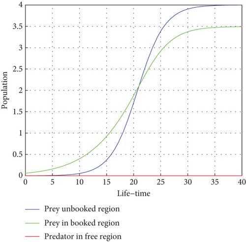
Figure 1 illustrates how there are fewer predators than prey, and the number of prey will rise. Within a population cycle of expansion and fall, these dynamics persist. Both prey populations are still bounded, and T = 27.21^°C indicates that, in the absence of predators, the migration rate of both prey regularly surpasses a certain threshold. This supports Theorem 1.

Details are in the caption following the image — **Figure 1 (a) Time series plot**
Open in figure viewer PowerPoint

Existence of prey population at the initial conditions (0.001,0.06,0.00) with parametric values r₁ = 0.5, r₂ = 0.2, μ = 0.5, δ = 0.06. (a) The stable case at E₂. (b) The periodic case.

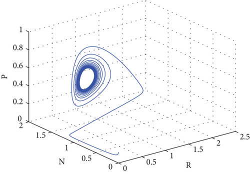
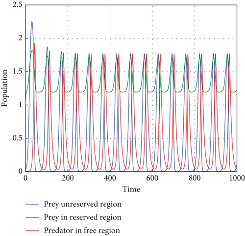
Here, we verify the fulfillment of the prerequisites outlined in Theorem 2, establishing the global asymptotic stability of the system. The established local stability along the solution branch serves as a tool to characterize the overall qualitative behavior of the system. In Figure 2, we depict the dynamics of the three populations based on the data provided at a temperature of T = 26.3^°C. This specific temperature condition allows the predator to coexist in the model system (1) with focal prey during periods of elevated temperatures and diminishing population growth rates.

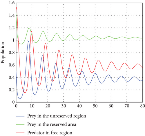
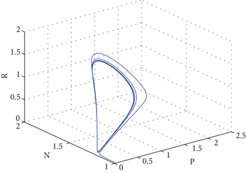
The most significant exogenous variable influencing predator populations on prey is temperature. There are two stages to the relationship between temperature and life history factors, such as development rate. The intrinsic growth rate of a population can be described as having a rise during the first stage, which takes place in the interval between some base and optimal temperature. Should this ideal temperature ever be surpassed, the population growth rate will decrease to zero at the highest point during the second stage. Using the parameters in the Table 2, we can comprehend Figure 2. Theorem 2 is verified first in this analysis, and E(P^∗, N^∗, R^∗) = (0.86,1.64,3.52) indicates the existence of the interior equilibrium point of the model system (1) with parameter values r₁(T) = 0.45, r₂(T) = 1.19604, δ = 0.06, μ(T) = 5.9.

Table 2. Parameter values of model system (1).

Parameters	Numerical values	References
α	0.2	[27]
k₁	100	[27]
k₂	10	[1]
δ	Variable	Estimation
β	0.15	[28]
c	0.5	[29]
T	[10°C, 27.21°C]	[17]
r(T)	Variable	Calculated depending on temperature (T)
μ(T)	Variable	Calculated depending on r(T)

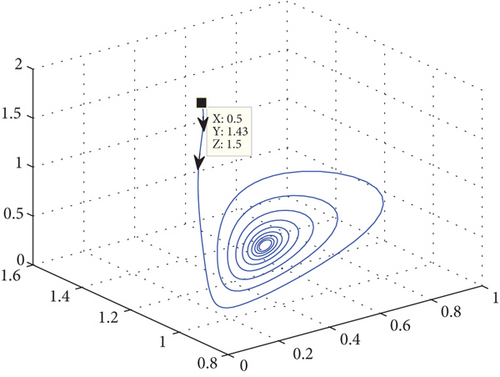
The oscillation behavior of the other interior equilibrium point is seen here in Figure 2. Figure 2 is the corresponding phase portrait which shows a stable limit cycle around the fixed point. We note that, because the initial value is taken near to E₂, the system achieves the attractor soon when the oscillation amplitudes for all time series have the same size, which is globally stable in Figure 3.

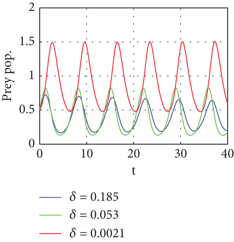
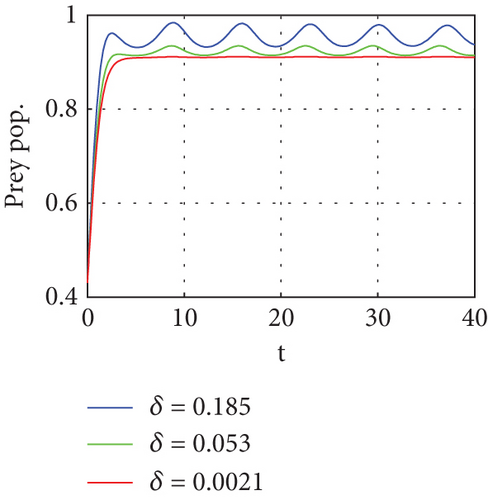
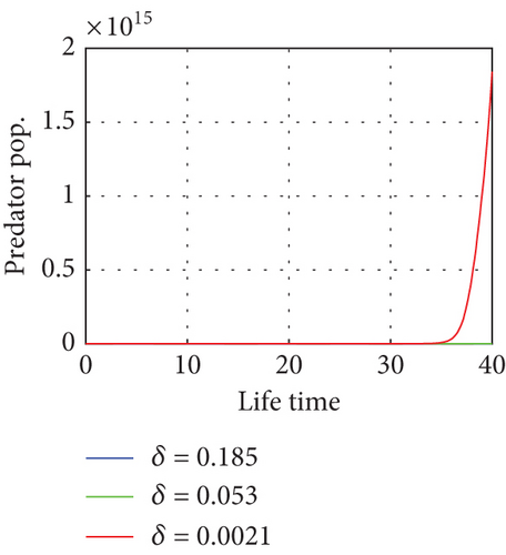
One effective strategy to safeguard the prey–predator system is to build a refuge zone; another is to give the predator more food. Predators stop attacking their prey when they have enough food, allowing the prey to live in the wild. The addition of food supplementation benefits the prey as well as the predator and is generally employed as a biological control tactic. Parameter δ is a significant metric that indicates the quantity of additional food. Thus, we carry out more research to learn how and influence system dynamics. We numerically simulate in multiple ways.

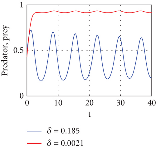
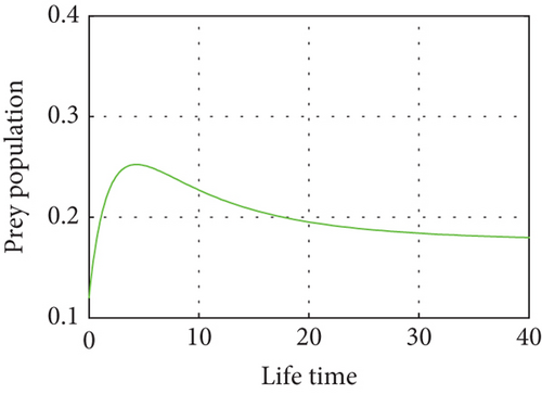
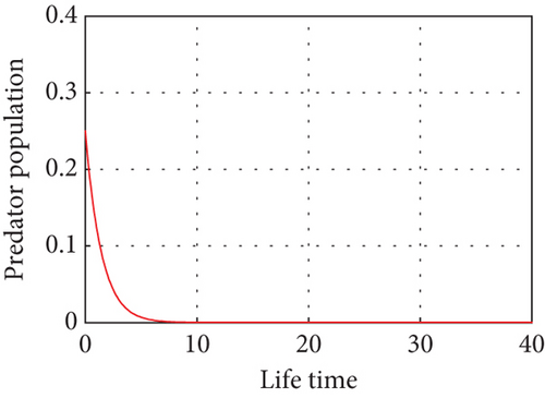
The interior equilibrium point of the system (1) is (0.72,0.012, 0.25), with parameter r₁ = 0.1, r₂ = 0.19, α = 0.5, μ = 0.2. We confirm that Theorem 1 is locally asymptotically stable. Look at Figure 4.

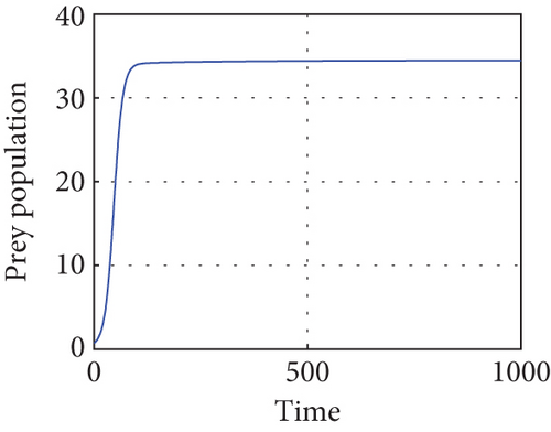
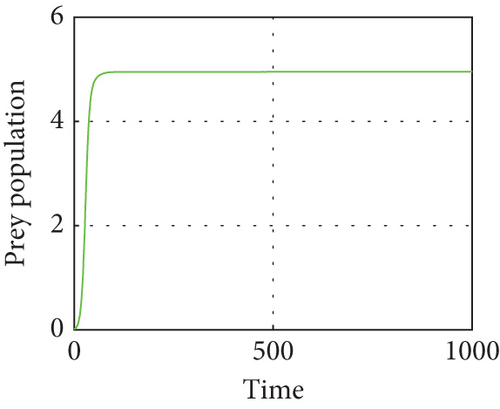
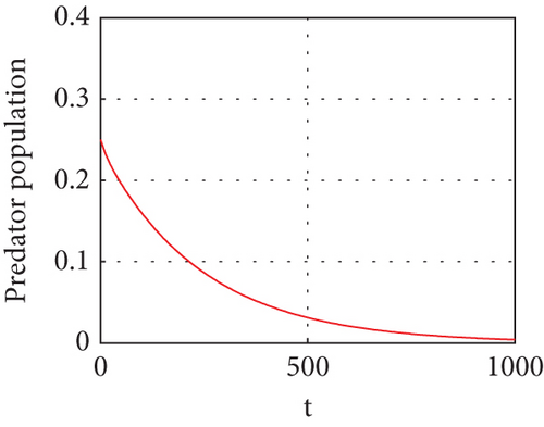
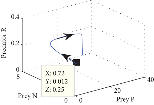
Figure 4 shows that prey populations are increasing as the decreasing of predator populations.

Figure 5 shows that if prey refugees increase, the predator population decreases. That is, prey is inversely proportional to the predator. Increases in the prey refugee can be due to drought (high temperature). Increasing temperature becomes more disturbance of the existing population. Consequently, increased prey refuge becomes a predator population that will die out.

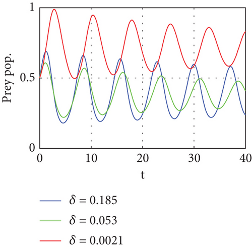
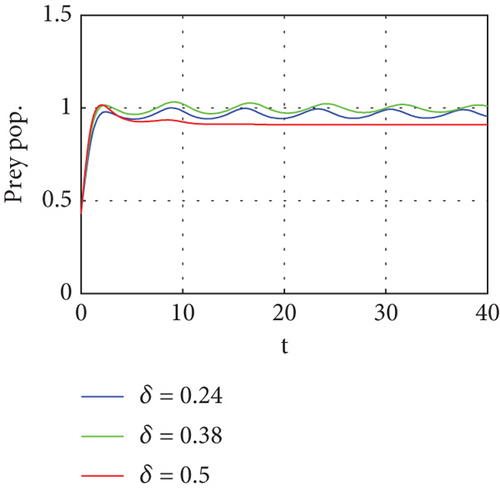
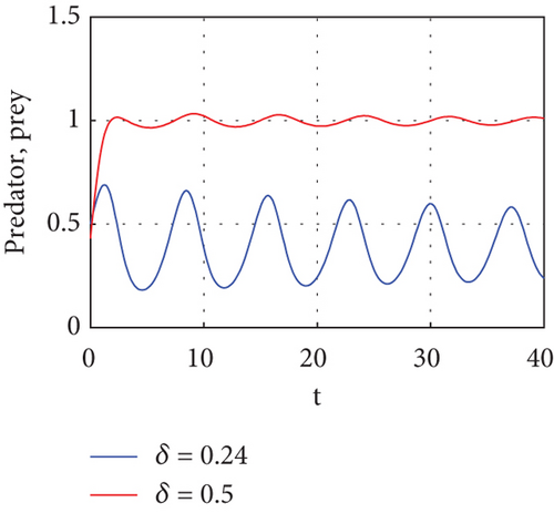
Figure 6 demonstrates that when prey refugee numbers decline, predator populations grow and have access to more food. Declines in prey refuge population size can be due to temperature balance. The stability range of predators increases gradually due to a decrease in prey refuge and an increase in prey in reserved areas.

The bifurcation parameters are summarized in Table 3.

Table 3. Bifurcation thresholds of parameters.

Bifurcation	Thresholds of parameters	Numerical values	References
Transcritical bifurcation	φ	0.1667
	γ	0.8333
	η	1, 1.8	[4]

Figure 7 illustrates the bifurcation diagram around the parameter η that shows the impact of prey population in the reserved area, and it confirms Theorem 5.

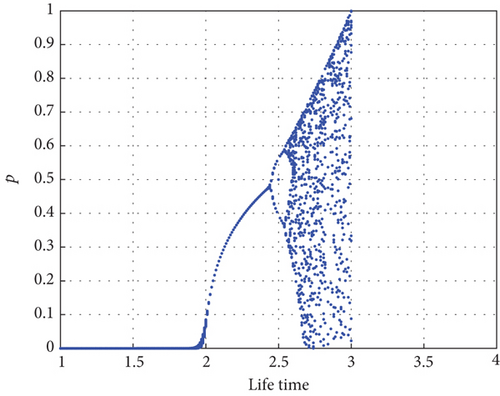
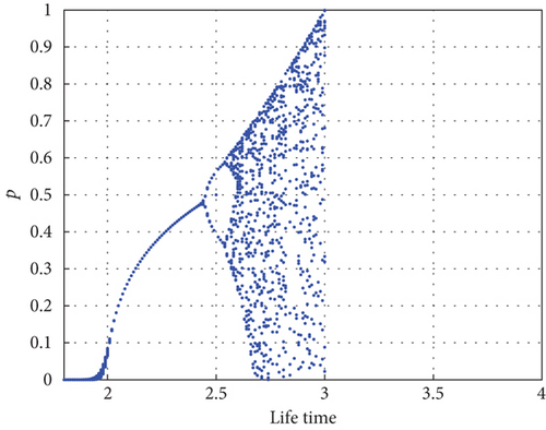
The bifurcation diagram shown in Figure 8 examines the impact of parameter η₁. Predator–prey interaction only displays equilibrium dynamics if the proportion δ of prey refuge is increased to 0.45, as determined from dimensionless data. The red color dash of Figure 8 indicates that the predator conversion is disruptive when the prey refuge is high. For η₁ < 0.45, there is an asymptotically stable equilibrium E₂, as shown by Proposition 4, which is indicated by a solid line (blue) where the red color curve in Figure 8 serves as the saddle point.

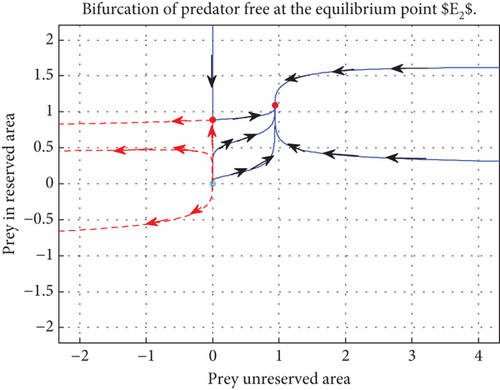
The main results indicate that refuge has a major impact on the stability of the system. Two strategies that work well to lessen the effects of prey refuge and maintain both predator and prey for their natural survival are the creation of refuge areas and the release of more food for predators. Although these methods are both positive and negative, improper application of them can lead to the extinction of a species in addition to maintaining its ongoing survival.

4.2. The Impact of Temperature on Predator–Prey Population

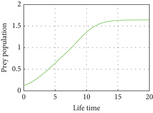
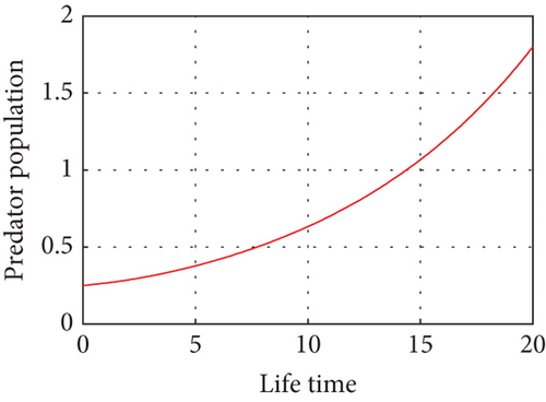
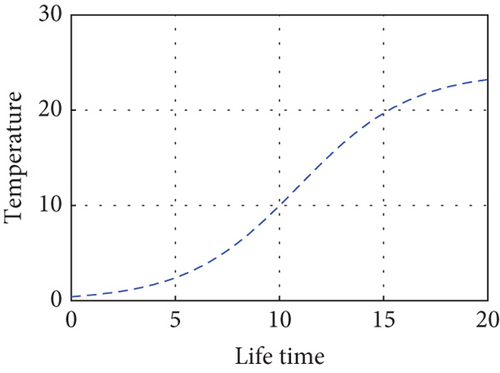
Climate change may impact populations in a number of ways, ranging from individual attributes to population-level impacts that may reshape predator–prey relationships. Climate-related temperature variations can affect a species’ developmental characteristics, particularly its behavior, which can influence how a predator–prey relationship plays out. Look at the following figures.

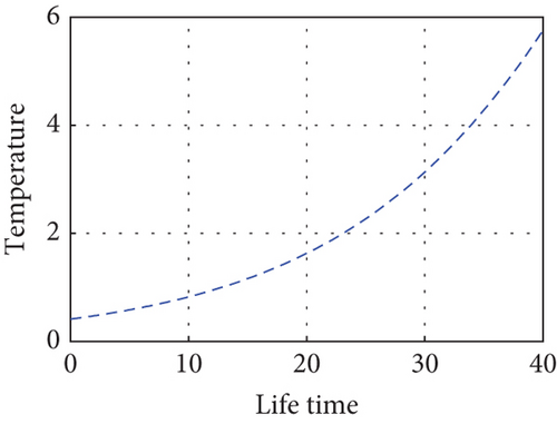
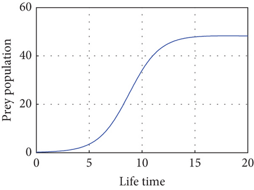
Here, we propose a conceptual model that explains how the relative performances of predators and prey affect the predator–prey populations’ temperature dependence. The predator population is declining as the temperature rises above (27.3°C) due to a lack of food sources and drought, and the prey population in the unreserved area is also declining as a result of climate variability, high temperatures (drought), and the prey reserved area gradually declining in the reserved area as shown in Figure 9. Drought-related climate change may alter predator–prey interactions by altering the spatial and temporal makeup of local communities. This demonstrates how predator–prey populations experience disruptions in their lives when temperatures are high during drought seasons. Populations may exhibit shifts in cyclic length or system stability in response to rising temperatures. The temperature balance is between 10°C and 26°C, and the predator population in the free region is growing modestly, in direct proportion to the increases in the prey population as shown in Figure 10.

5. Conclusion

In conclusion, our study highlights the crucial role of refuges in the biological regulation of predator–prey populations. Expanding refuges, however, may lead to higher prey densities and population epidemics, particularly in hotspot regions qualified as refugia where predators struggle to subdue prey effectively. The solution to our model asymptotically approaches its equilibrium level in the interior of for various values of δ, indicating the significance of migration to reserved regions. As a result of many predator–prey groups actually having access to some kind of shelter, the model becomes more realistic when refuge is added to the system (1). While prey immigration can lessen the chance of extinction due to predation, much like sanctuary does, predator immigration can help manage prey populations and preserve predator populations. From our perspective, the models are significant because they provide a theoretical framework and a way to assess the effects of adding temperature dependency to the intrinsic growth rate.

Indeed, the intrinsic growth rate of the prey population as a function of temperature is represented by the parameters r₁(T) and r₂(T), which have been taken to be constant. Following completion of the work described in this study, we included a temperature-dependent relationship for μ(T). This relationship was derived from relevant parameter values in a manner similar to determining the temperature-dependent values of r₁(T) and r₂(T). Consequently, it makes sense to conclude that the temperature-dependent regions that are important to the population dynamics of the system are the relationships shown in Figures 1 and 4. We present quantitative evidence in favor of the hypothesis that the equilibrium density of prey decreases while that of predators rises as prey refuges grow. In actuality, predator equilibrium density rises and then falls as prey refuges increase.

Furthermore, varying the parameter δ, representing the impact of the unreserved region on population behavior, influences the system’s solution near the equilibrium point. Decreasing δ, indicative of abundant prey, negatively impacts predator density. These findings contribute to our understanding of how environmental factors, refuge dynamics, and population behavior interact in complex ecological systems.

Conflicts of Interest

The authors declare no conflicts of interest.

Author Contributions

Negeri Negese Wayesa: methodology, software, formal analysis, investigation, writing—original draft, writing—review and editing. Legesse Lemecha Obsu: conceptualization, methodology, validation, formal analysis, investigation, writing—review and editing, supervision. Mohammed Yiha Dawed: conceptualization, investigation, validation, formal analysis, writing review and editing, supervision.

Funding

The authors received no specific funding for this work.

Acknowledgments

The authors thank Bule Hora University for its hospitality and support during this work.

Open Research

Data Availability Statement

The data utilized in this study are provided within the manuscript itself.

References

1 Mondal N., Alrabaiah H., Barman D., Roy J., and Alam S., Influence of predator incited fear and interference competition in the dynamics of prey-predator system where the prey species are protected in a reserved area, Ecol Environmental Conservation. (2022) 28, 831–852.
10.53550/EEC.2022.v28i02.040
Google Scholar
2 Selwood K. and Zimmer H., Refuges for biodiversity conservation: a review of the evidence, Biological Conservation. (2020) 245, article 108502, https://doi.org/10.1016/j.biocon.2020.108502.
10.1016/j.biocon.2020.108502
Web of Science® Google Scholar
3 DeMarche M. L., Doak D. F., and Morris W. F., Incorporating local adaptation into forecasts of species’ distribution and abundance under climate change, Global Change Biology. (2019) 25, no. 3, 775–793, https://doi.org/10.1111/gcb.14562, 2-s2.0-85060657685, 30597712.
10.1111/gcb.14562
PubMed Web of Science® Google Scholar
4 Nunez S., Arets E., Alkemade R., Verwer C., and Leemans R., Assessing the impacts of climate change on biodiversity: is below 2°C% enough?, Climatic Change. (2019) 154, no. 3-4, 351–365, https://doi.org/10.1007/s10584-019-02420-x, 2-s2.0-85066913440.
10.1007/s10584-019-02420-x
Web of Science® Google Scholar
5 Luna-Aranguré C. and Vázquez-Domínguez E., Analysis of the application of ecological niche modeling in phylogeographic studies: contributions, challenges, and future, Therya. (2020) 11, no. 1, 47–55, https://doi.org/10.12933/therya-20-844.
10.12933/therya-20-844
Google Scholar
6 Helmuth B., Broitman B. R., Blanchette C. A., Gilman S., Halpin P., Harley C. D., O′Donnell M. J., Hofmann G. E., Menge B., and Strickland D., Mosaic patterns of thermal stress in the rocky intertidal zone: implications for climate change, Ecological Monographs. (2006) 76, no. 4, 461–479, https://doi.org/10.1890/0012-9615(2006)076%5b0461:MPOTSI%5d2.0.CO;2, 2-s2.0-33845336136.
10.1890/0012-9615(2006)076[0461:MPOTSI]2.0.CO;2
Web of Science® Google Scholar
7 Currie-Olsen D., Hesketh A. V., Grimm J., Kennedy J., Marshall K. E., and Harley C. D., Lethal and sublethal implications of low temperature exposure for three intertidal predators, Journal of Thermal Biology. (2023) 114, article 103549, https://doi.org/10.1016/j.jtherbio.2023.103549, 37244058.
10.1016/j.jtherbio.2023.103549
PubMed Web of Science® Google Scholar
8 Bastille-Rousseau G., Schaefer J. A., Peers M. J., Ellington E. H., Mumma M. A., Rayl N. D., Mahoney S. P., and Murray D. L., Climate change can alter predator–prey dynamics and population viability of prey, Oecologia. (2018) 186, no. 1, 141–150, https://doi.org/10.1007/s00442-017-4017-y, 2-s2.0-85034661655, 29167983.
10.1007/s00442-017-4017-y
PubMed Web of Science® Google Scholar
9 Webber Q. M., Albery G. F., Farine D. R., Pinter-Wollman N., Sharma N., Spiegel O., Vander Wal E., and Manlove K., Behavioural ecology at the spatial–social interface, Biological Reviews. (2023) 98, no. 3, 868–886, https://doi.org/10.1111/brv.12934, 36691262.
10.1111/brv.12934
PubMed Web of Science® Google Scholar
10 Manríquez P. H., Jara M. E., González C. P., Seguel M. E., Domenici P., Watson S.-A., Anguita C., Duarte C., and Brokordt K., The combined effects of climate change stressors and predatory cues on a mussel species, Science of the Total Environment. (2021) 776, article 145916, https://doi.org/10.1016/j.scitotenv.2021.145916, 33639464.
10.1016/j.scitotenv.2021.145916
PubMed Web of Science® Google Scholar
11 Lafferty K. D., The ecology of climate change and infectious diseases, Ecology. (2009) 90, no. 4, 888–900, https://doi.org/10.1890/08-0079.1, 2-s2.0-63849101815.
10.1890/08-0079.1
PubMed Web of Science® Google Scholar
12 Pal S., Panday P., Pal N., Misra A., and Chattopadhyay J., Dynamical behaviors of a constant prey refuge ratio-dependent prey-predator model with Allee and fear effects, International Journal of Biomathematics. (2024) 17, no. 1, https://doi.org/10.1142/S1793524523500109.
10.1142/S1793524523500109
Web of Science® Google Scholar
13 Orrock J. L., Preisser E. L., Grabowski J. H., and Trussell G. C., The cost of safety: refuges increase the impact of predation risk in aquatic systems, Ecology. (2013) 94, no. 3, 573–579, https://doi.org/10.1890/12-0502.1, 2-s2.0-84876144252, 23687883.
10.1890/12-0502.1
PubMed Web of Science® Google Scholar
14 Alabacy Z. K. and Majeed A. A., The fear effect on a food chain prey-predator model incorporating a prey refuge and harvesting, Journal of physics: Conference series. (2021) 1804, article 012077.
Google Scholar
15 Loko O. P., Nwagor P., and Georqe I., A simulation study of predator-prey interaction model with changing climatic factors in an aquatic environment, Faculty of Natural and Applied Sciences Journal of Scientific Innovations. (2023) 4, no. 1, 211–220.
Google Scholar
16 Mandal G., Ali N., Guin L. N., and Chakravarty S., Impact of fear on a tri-trophic food chain model with supplementary food source, International Journal of Dynamics and Control. (2023) 11, no. 5, 2127–2160, https://doi.org/10.1007/s40435-022-01104-2.
10.1007/s40435-022-01104-2
Google Scholar
17 Collings J. B., Bifurcation and stability analysis of a temperature-dependent mite predator-prey interaction model incorporating a prey refuge, Bulletin of Mathematical Biology. (1995) 57, no. 1, 63–76, https://doi.org/10.1016/0092-8240(94)00024-7, 7833852.
10.1016/0092-8240(94)00024-7
CAS PubMed Web of Science® Google Scholar
18 Wollkind D. J., Collings J. B., and Logan J. A., Metastability in a temperature-dependent model system for predator-prey mite outbreak interactions on fruit trees, Bulletin of Mathematical Biology. (1988) 50, no. 4, 379–409, https://doi.org/10.1016/S0092-8240(88)90005-5.
10.1016/S0092-8240(88)90005-5
Web of Science® Google Scholar
19 Jana A. and Roy S. K., Fostering roles of super predator in a three-species food chain, International Journal of Dynamics and Control. (2023) 11, no. 1, 78–93, https://doi.org/10.1007/s40435-022-00970-0.
10.1007/s40435-022-00970-0
Google Scholar
20 Dawed M. Y. and Kebedow K. G., Coexistence and harvesting optimal policy in three species food chain model with general Holling type functional response, Natural Resource Modeling. (2021) 34, no. 3, article e12316, https://doi.org/10.1111/nrm.12316.
10.1111/nrm.12316
Web of Science® Google Scholar
21 Ashine A. B. and Gebru D. M., Mathematical modeling of a predator-prey model with modified Leslie-Gower and Holling-type Ii schemes, Mathematics and Decision Sciences. (2017) 17, 20–40.
Google Scholar
22 Abdul Satar H. and Naji R. K., Stability and bifurcation of a prey-predator-scavenger model in the existence of toxicant and harvesting, International Journal of Mathematics and Mathematical Sciences. (2019) 2019, 17, https://doi.org/10.1155/2019/1573516, 2-s2.0-85064341503, 1573516.
10.1155/2019/1573516
Google Scholar
23 Ma Z., Wang S., Wang T., and Tang H., Stability analysis of prey-predator system with holling type functional response and prey refuge, Advances in Difference Equations. (2017) 2017, no. 1, 12, https://doi.org/10.1186/s13662-017-1301-4, 2-s2.0-85027676660.
10.1186/s13662-017-1301-4
Google Scholar
24 Al-Momen S. and Naji R. K., The dynamics of modified Leslie-Gower predator-prey model under the influence of nonlinear harvesting and fear effect, Iraqi Journal of Science. (2022) 63, 259–282, https://doi.org/10.24996/ijs.2022.63.1.27.
10.24996/ijs.2022.63.1.27
Google Scholar
25 Freedman H. I. and Waltman P., Persistence in models of three interacting predator-prey populations, Mathematical Biosciences. (1984) 68, no. 2, 213–231, https://doi.org/10.1016/0025-5564(84)90032-4, 2-s2.0-48749138514.
10.1016/0025-5564(84)90032-4
Web of Science® Google Scholar
26 Zhao J. and Shao Y., Bifurcations of a prey-predator system with fear, refuge and additional food, Mathematical Biosciences and Engineering. (2023) 20, no. 2, 3700–3720, https://doi.org/10.3934/mbe.2023173, 36899600.
10.3934/mbe.2023173
PubMed Web of Science® Google Scholar
27 Zhang H., Cai Y., Fu S., and Wang W., Impact of the fear effect in a prey-predator model incorporating a prey refuge, Applied Mathematics and Computation. (2019) 356, 328–337, https://doi.org/10.1016/j.amc.2019.03.034, 2-s2.0-85063610028.
10.1016/j.amc.2019.03.034
Web of Science® Google Scholar
28 Abdulghafour A. S. and Naji R. K., Modeling and analysis of a prey-predator system incorporating fear, predator-dependent refuge, and cannibalism, Communications in Mathematical Biology and Neuroscience. (2022) 2022.
Google Scholar
29 Melese D., Muhye O., and Sahu S. K., Dynamical behavior of an eco-epidemiological model incorporating prey refuge and prey harvesting, Applications and Applied Mathematics: An International Journal (AAM). (2020) 15, no. 2.
Web of Science® Google Scholar

Citing Literature

All articles

Analysis of Predator–Prey Model With Inclusion of Temperature Variability in Prey Refugees

Abstract

1. Introduction

2. Mathematical Model Formulation

2.1. Model Assumptions

3. Model Analysis

3.1. Positivity, Uniqueness, and Boundedness of Solution

3.1.1. Positivity of the Solution

3.1.2. Boundedness of Solutions of the Model System

3.1.3. Uniqueness

3.2. Existence of Equilibrium Points

3.3. Local Stability of the Equilibrium Point

3.4. Global Stability

3.5. Persistence

3.6. Local Bifurcation Analysis

4. Numerical Simulation

4.1. Simulation Results

4.2. The Impact of Temperature on Predator–Prey Population

5. Conclusion

Conflicts of Interest

Author Contributions

Funding

Acknowledgments

Open Research

Data Availability Statement

References

Citing Literature

Figures

References

Information

About Wiley Online Library

Help & Support

Opportunities

Connect with Wiley

Analysis of Predator–Prey Model With Inclusion of Temperature Variability in Prey Refugees

Abstract

1. Introduction

2. Mathematical Model Formulation

2.1. Model Assumptions

3. Model Analysis

3.1. Positivity, Uniqueness, and Boundedness of Solution

3.1.1. Positivity of the Solution

3.1.2. Boundedness of Solutions of the Model System

3.1.3. Uniqueness

3.2. Existence of Equilibrium Points

3.3. Local Stability of the Equilibrium Point

3.4. Global Stability

3.5. Persistence

3.6. Local Bifurcation Analysis

4. Numerical Simulation

4.1. Simulation Results

4.2. The Impact of Temperature on Predator–Prey Population

5. Conclusion

Conflicts of Interest

Author Contributions

Funding

Acknowledgments

Open Research

Data Availability Statement

References

Citing Literature

Figures

References

Related

Information