In this study, we consider a parameter-uniform convergent numerical approach for a class of time-fractional singularly perturbed partial differential equations (TF-SPDPDEs) with large delay in time that exhibits a regular exponential boundary layer on the right side of the spatial domain. An arbitrary very small parameter ε(0 < ε < <1) multiplies the highest-order derivative term of these singularly perturbed problems. The time-fractional derivative is considered in the Caputo sense with order α ∈ (0, 1). The numerical scheme comprises the L1 scheme and nonstandard finite difference method (FDM) for discretizing the time and space variables, respectively, on a uniform mesh. To show the parameter uniform convergence of the proposed method, the truncation error and stability analysis are discussed. The method is shown to be parameter-uniform convergent of order O((Δt)^2−α + Δx), where Δt and Δx are the step sizes in the time and space directions, respectively. In order to confirm the theoretical predictions, two numerical examples are presented, and the numerical results support the theoretical concepts discussed. Finally, to show the advantage of the proposed scheme, we made comparisons with the existing numerical methods in the literature, and the numerical results reveal that the present scheme is more accurate.

1. Introduction

In different fields of science and engineering, we frequently encounter partial differential equations (PDEs) whose solutions have a multiscale property. This means that in some regions of the domain, the solution behaves smoothly and abruptly in other regions. PDEs that have this property are said to be singularly perturbed PDEs (SPPDEs). The regions where the solution changes abruptly are the inner and/or boundary layer regions, and the parts of the domain where the solution behaves smoothly are the outer regions. If such a rapid change occurs at the boundary of the domain, then the phenomenon is said to be a boundary layer phenomenon. Mathematically, the PDE is singularly perturbed when the perturbation parameter (ε) multiplies the highest-order derivative. This leads to the solution of the SPPDE being qualitatively different from the solution of the unperturbed problem when we set ε = 0. SPPDEs are applicable in various branches of science and engineering, such as in fluid dynamics, quantum mechanics, chemical reactor theory, elasticity, and the theory of porous gas electrodes [1].

Due to the influence of the perturbation parameter, standard numerical methods, such as the finite difference method (FDM), finite element method (FEM), finite volume method (FVM), and collocation method, fail to solve SPPDEs, and unacceptably large oscillations occur in the boundary layer region, unless the mesh discretization used is extremely fine, which is computationally expensive and not practical. To avoid this problem, one needs to use parameter-uniform convergent numerical methods to solve SPPDEs. In the literature, there are two popular uniformly convergent numerical methods for solving SPPDEs in the context of FDMs [2]. They are fitted operator method (FOM) and fitted mesh method (FMM). FOM controls the rapid (abrupt) change of the solution in the boundary layer region by introducing a fitting factor or denominator function on the term containing the singular perturbation parameter with a uniform mesh, whereas FMM uses fine meshes in the boundary layer region and coarse meshes in the region away from the boundary layer (outer region). FMMs are defined on piecewise uniform meshes. FOM can be divided into two groups: the exponentially fitted operator FDM (EFOFDM) and the nonstandard FDM (NSFDM). NSFDM controls the rapid growth of the solution of SPPDEs in the boundary layer region by replacing the denominator of the classical second-order central finite difference approximation of the second-order derivative with a positive function constructed systematically using Mickens rules [3].

In recent decades, fractional calculus has gained great emphasis due to its wide applications in many areas of science and engineering, such as in fluid flow problems with a porous medium, anomalous transport in cell biology, oil industry, neural networks, mass transfer in fluids, feedback control system, finance, and viscoelasticity material [4–8]. It is the study of arbitrary-order derivatives and integrals. Since fractional-order derivative and integral operators have nonlocal characteristics, it is confirmed that they can accurately model the memory effect and the hereditary properties of certain complex systems with anomalous dynamics [9], which are neglected in integer-order derivative and integral operators. There are different definitions of fractional derivatives such as Riemann–Liouville, Riesz, Caputo, Grunwald–Letnikov, Marchaud, Weyl, and Sonin–Letnikov. In this paper, we used the Caputo fractional derivative because it allows the traditional initial and boundary conditions with a known physical interpretation. The PDEs that contain fractional-order derivatives are classified into two groups [10]. They are space-fractional PDEs (SF-PDEs) and time-fractional PDEs (TF-PDEs). Specifically, a TF-PDE can be used to model the time-related anomalous dynamics, which is widely used in oil reservoir simulations, transport of mass and energy dispersion of chemicals in reactors, and so on [11].

In contrast to classical PDEs, which model physical problems only at the current instant, delay PDEs (DPDEs) and time-fractional DPDEs (TF-DPDEs) are used to simulate physical problems for which the future state depends on both the present state and the past history of the system. They give more realistic models for many problems in science and engineering. For this reason, one cannot neglect the delay term, despite the whole history being considered by time-fractional differential equations [10]. Moreover, TF-DPDEs that contain a perturbation parameter are said to be time-fractional singularly perturbed DPDEs (TF-SPDPDEs). Due to the nonlocal property of the time-fractional derivative and the involvements of the perturbation and delay parameters, it is very difficult to find the exact solutions of TF-SPDPDEs. Therefore, we need to find at least an approximate solution using a numerical method that converges uniformly with respect to the perturbation parameter ε.

During the past few decades, various semianalytical methods have been used, such as the Laplace transform method [12], Fourier transform method [13], Adomian decomposition method [14], homotopy perturbation method [15], variational iteration method [16], and generalized differential transform method [17], and numerical methods such as the FDM [18–20], FEM [21], operational matrix method [22], and collocation method [23] have been introduced to solve FPDEs. For instance, Choudhary, Singh, and Kumar [10] proposed a numerical method for a class of TF-PDEs with delay in time. The numerical method comprises the Crank–Nicolson method for the uniformly discretized time domain and the Spline method with a tension factor in the spatial domain. Rihan [24] presented θ-method to solve linear and nonlinear TF-DPDEs. However, the problems considered in the above work are not singularly perturbed. Relatively, if the problems are not singularly perturbed (in the absence of the perturbation parameter), we may not have numerical difficulties to solve.

Within the past 20 years, many scholars have been studied on numerical treatment of classical (integer-order) singularly perturbed DPDEs (e.g., see [25–34] and the references therein). However, the numerical treatments of the TF-SPDPDEs are still at the initial stage. The scholars Sahoo and Gupta in [35] designed a parameter uniformly convergent numerical scheme for a class of time-fractional singularly perturbed convection–diffusion problems without a delay term that exhibits a weak initial layer at the initial time t = 0 and an exponential boundary layer on the right side of the spatial domain as ε⟶0. They discretized the time-fractional derivative using a classical L1 scheme on a graded mesh and a piecewise uniform Shishkin mesh to the space derivatives. Similarly, these authors in [36] developed a robust higher-order uniformly convergent numerical scheme to solve the same problem. The authors employed Alikhanovs L2 − 1_σ approximation in the temporal direction on a graded mesh, and the space domain is discretized on a piecewise uniform Shishkin mesh using a combination of midpoint upwind and central finite difference operators. Liu et al. [11] designed a stable numerical scheme to solve time-fractional SPPDEs with variable coefficients. They employed the tailored finite-point method to approximate the space derivative and the Grunwald–Letnikov and L1 schemes to approximate the time-fractional derivative. Kumie, Tiruneh, and Derese in [37] employed the Crank–Nicolson method combined with the NSFDM for solving TF-SPDPDEs. The authors Aniley and Duressa in [38] presented the NSFDM to solve the time-fractional singularly perturbed convection–diffusion problems with a delay in time. The time-fractional and space derivatives are discretized by using the Crank–Nicolson and NSFDMs, respectively, on a uniform mesh. The scholars Kumar, Podila, and Vigo-Aguiar in [39] developed a parameter uniformly convergent numerical scheme to obtain an approximate solution of time-fractional SPPDEs with delay in time. They used the L1 scheme on a uniform mesh to approximate the time-fractional derivative and the stable FDM with piecewise uniform meshes (which are adequate for FMMs) to approximate the spatial derivatives. Motivated by the study of Kumar, Podila, and Vigo-Aguiar in [39], in this work, this study is aimed at designing a parameter uniformly convergent numerical method with a better accuracy to solve the time-fractional SPPDEs with a large delay in time, which is given in Equations (1) and (2). To approximate the time-fractional and space derivatives, we employed the L1 scheme and NSFDM, respectively, on a uniform mesh. NSFDM, which is one of the FOMs, has an advantage over FMM that is easy to implement and does not require any priori information about the location and width of the boundary layer(s) [40]. The advantage of the proposed method is to develop more accurate parameter uniformly convergent numerical scheme to solve time-fractional SPPDEs with large time delay.

The remaining parts of the paper are structured as follows: Problem formulation appears in Section 2. Section 3 describes the numerical discretization of the continuous problem. In Section 4, we show the convergence analysis of the fully discrete scheme. Numerical examples and results are presented in Section 5, which validates the theoretical results. The article ends with Section 6, which is devoted to the conclusion.

In this paper, C represents a positive constant independent of the perturbation parameter, grid points, and step sizes. Here, ‖.‖_Ω denotes the maximum norm, which is defined by

( )

for a function g defined on some domain Ω.

2. Formulation of the Continuous Problem

Consider the following one-dimensional time-fractional SPPDE with a large delay in time defined on the rectangular domain

in the x − t plane:

(1)

with interval and boundary conditions:

(2)

where 0 < ε < <1 denotes the perturbation parameter, τ > 0 denotes the delay parameter, and the boundary of the domain is Γ = Γ_l ∪ Γ_b ∪ Γ_r. The time-fractional derivative ∂^αu(x, t)/∂t^α is given in the Caputo sense with order α ∈ (0, 1), usually denoted by

and defined by

( )

where Γ represents the gamma function defined as for z ∈ ℂ with Re(z) > 0,

( )

Suppose p(x) ≥ ρ > 0, q(x, t) ≥ β > 0, r(x, t) ≥ γ > 0, and f(x, t) are bounded and sufficiently smooth functions on the domain

. In addition, let us also assume that the given initial and boundary functions satisfy the following compatibility condition at the corner points of

(i.e., at (0,0) and (1,0)). This means

( )

Under these assumptions imposed on the functions ψ_b(x, t), ψ_l(t), ψ_r(t), and f at the corners of Ω, the interval boundary value problem (Equations (1) and (2)) admits a unique solution u(x, t) that exhibits a regular exponential boundary layer of width O(ε) at x = 1 of Ω, when the perturbation parameter becomes very small (ε⟶0). Because of the nonlocality (long memory) of the fractional-order derivative and the model problem contains the delay and perturbation parameters, it is a difficult task to solve singularly perturbed TF-PDEs effectively and accurately. Hence, designing simple and more accurate ε-uniform convergent numerical methods (i.e., methods whose accuracy does not depend on the perturbation parameter) for such problems is an important task and is the objective of this study.

2.1. Properties of the Continuous Problem

In this subsection, we describe some properties of the continuous problem given in Equations (1) and (2) that ensure the applicability of the maximum principle for the stability estimate of its analytical solution. These properties are essential for analyzing the numerical schemes of the semi- and fully discrete problems, which we will present in the next sections.

Lemma 1 (continuous maximum principle). Let satisfy Φ(x, t) ≥ 0, ∀(x, t) ∈ Γ and . Then, .

Proof 1. The proof of this lemma can be done by contradiction. Suppose such that

( )

and assume that Φ(x^⋆, t^⋆) < 0. From the hypothesis, we have (x^⋆, t^⋆) ∉ Γ as Φ ≥ 0 on Γ and (x^⋆, t^⋆) ∈ Ω. As it attains minimum at (x^⋆, t^⋆), we have ∂Φ(x^⋆, t^⋆)/∂x = 0, ∂²Φ(x^⋆, t^⋆)/∂x² ≥ 0 and

(by extremum principle for the Caputo fractional derivative [41]), and since q(x^⋆, t^⋆) ≥ 0, we have

( )

which contradicts the assumption

in Ω. Hence, Φ(x^⋆, t^⋆) ≥ 0. Therefore, we conclude that

Lemma 2. The solution of the continuous problem given in Equations (1) and (2) satisfies the following estimate:

( )

Proof 2. Using the smoothness and compatibility conditions of the solution of the continuous problem (Equation (1)) at the corner points (i.e., (0,0) and (1,0)) and the continuous maximum principle given in Lemma 1 on the barrier functions defined by

( )

give the required estimate. To show this, we have

( )

On the boundary Γ_b,

( )

Additionally, for (x, t) ∈ Ω,

( )

since C can be chosen sufficiently large.

Thus, by using the continuous maximum principle given in Lemma 1, we obtain

( )

This implies that

( )

Lemma 3. Let u(x, t) be the solution of the problem (Equations (1) and (2)). Then, we have

( )

Proof 3. For every , we have the following:

( )

Since |ψ_b(x, 0)| is bounded and using Lemma 2, we obtain the desired result.

Lemma 4 (stability estimate of the continuous problem). Let u(x, t) be the solution of the problem (Equations (1) and (2)). Then, we have

( )

Proof 4. Define the barrier functions

( )

Thus, we have

( )

Also, for (x, t) ∈ Γ_b,

( )

Moreover, for (x, t) ∈ Ω,

( )

Therefore, by using Lemma 1, we get the required result.

3. Numerical Scheme

In this section, we derive a parameter uniformly convergent numerical scheme to approximate the continuous problem given in Equations (1) and (2) by discretizing both the time and space variables with a uniform mesh. To construct the scheme, we first discretize the temporal variable using the L1 scheme. Next, the semidiscretized problem is numerically approximated by using the NSFDM with a simple upwind scheme in the spatial direction.

3.1. Time Discretization

The use of Taylor’s series expansion for the terms containing delay in Equation (1) is invalid when the delay parameter τ is greater than the perturbation parameter ε. As a result, we first descretize the time domain [0, T] into N intervals with uniform step size Δt = T/N. Choosing k in such a way that τ = kΔt and for some positive integer k ∈ (0, N), we have

( )

We can construct the L1 scheme to approximate the Caputo time-fractional derivative

by using linear interpolation formula for the first-order derivative in the following way.

( )

Here, the coefficients b_j, j = 0, 1, ⋯, N − 1 are given by b_j = (j + 1)^1−α − j^1−α and

( )

Now, the term R is the truncation error and approximated by

(3)

Hence, the L1 scheme for the Caputo fractional derivative

is given by

(4)

Neglecting the truncation error from Equation (4) and since b₀ = 1, then the L1 approximation formula for the Caputo fractional derivative is

(5)

Evaluating Equation (1) on both sides at t = t_j and substituting Equation (5), we obtain the following equation:

( )

where

represents the approximate solution of u(x, t_j) at the j^th time level. Rearranging the above semidiscretized problem, we obtain the following:

(6)

(7)

Using semi-discrete differential operator

, Equation (6) can be written as

, where

(8)

(9)

(10)

Using the given interval condition, Equation (9) can be written as

(11)

The semidiscrete operator given in Equation (8) satisfies the following discrete maximum principle.

Lemma 5. Let be a smooth function on . If and , then .

Proof 5. To prove this lemma, we use proof by contradiction technique. Let such that

( )

and assume that

. From the hypothesis, we have x^⋆ ∉ {0, 1},

and since v(x^⋆, t_j) > 0, we have

( )

which is a contradiction to our assumption of

in Ω_x. This shows that our assumption is wrong and then

. Therefore, we conclude that

Theorem 1. Under the smoothness and compatibility conditions, the semidiscretized solution and its derivatives of the problems (Equations (6) and (7)) satisfy the following bounds:

( )

Proof 6. The proof is found in [42].

3.2. Spatial Discretization

Here, we will consider the spatial discretization of Equation (8) by the NSFDM on a uniform mesh. Let M be a positive integer and divide the domain [0, 1] into equal subdivisions M with step size Δx = 1/M in the x direction. Then, we have

( )

We will apply the NSFDM to discretize the space derivative using the principles of Mickens [3]. Consider the following second-order ordinary differential equation with constant coefficient by neglecting the time variable as

(12)

where p(x) ≥ β and v(x) ≥ θ. Hence, the problem given in Equation (12) has two linearly independent solutions, namely, exp(λ₁x) and exp(λ₂x), with

( )

If we denote the approximate solution of

at x_i by U_i, then the general solution of the problem given in Equation (12) at the grid point x_i is given by U_i = A₁exp(λ₁x_i) + A₂exp(λ₂x_i). Using the procedures used in [3], we have

(13)

Evaluating the determinant in Equation (13) and simplifying, we obtain

(14)

which is the difference approximation of the continuous problem given in Equation (12). After performing some computations and rearranging, we obtain the following:

(15)

Now, take the denominator function

Applying the variable coefficient p(x_i) = p_i to this denominator function, we write it as

(16)

Let U_i,j represent the approximation of

. Using the positive function given in Equation (16) as the denominator function to approximate the second-order derivative and a simple upwind finite difference approximation for the first derivative of Equation (8), we obtain the following fully discrete problem:

(17)

with interval boundary conditions:

(18)

The scheme obtained by replacing the denominator of the second-order central finite difference approximation of the second-order derivative by a positive function is said to be the method of nonstandard finite difference.

Rearranging Equation (17), we obtain the following tridiagonal linear system:

(19)

We can write the equation given in Equation (19) in matrix form:

(20)

where the matrix A is the tridiagonal matrix of size (M − 1) × (M − 1) given by

( )

Lemma 6 (fully discrete maximum principle). Assume that the discrete function Φ(x_i, t_j) satisfies Φ(x_i, t_j) ≥ 0 on (x_i, t_j) ∈ Γ^M,N and in . Then, Φ(x_i, t_j) ≥ 0, for all .

Proof 7. We can prove this by contradiction. Let s, s^⋆ be an index such that

( )

Then, by the given hypothesis, we have 0 < s < M and 0 < s^⋆ < N. It follows that . Hence,

( )

which is a contradiction to our assumption. Therefore,

An immediate consequence of Lemma 6 is the uniform stability estimate given below.

Lemma 7. The solution U_i,j of the fully discretized problem in (17) satisfy the following bound:

( )

Proof 8. To prove this lemma, let as denote

( )

and define the barrier function

At the boundary points,

( )

On the discretized domain x_i, i = 1, 2, ⋯, N − 1, we have

( )

By Lemma 6, we obtain , for all . This implies that

( )

In the next section, we estimate the error associated with the spatial discretization and convergence analysis of the presented scheme.

4. Convergence Analysis of the Fully Discrete Scheme

From Lemma 6 and Lemma 7, we proved that the fully discrete operator

satisfies the discrete maximum principle and the uniform stability estimate. In this section, we estimate the truncation error of the fully discrete problem. If U_i,j denotes the approximate solution in the fully discretization of the exact solution u(x, t) at (x_i, t_j), i = 0, 1, ⋯, M, j = 0, 1, ⋯, N, then the truncation error of the scheme (Equations (17) and (18)) is given by

(21)

Next, we need to show that

is bounded. To show this, let as denote ρ = p_iΔx/ε, ρ ∈ (0, ∞). Then, we obtain the relation as derived in [43]

( )

Simplifying and explicitly writing, we obtain

( )

Then, we have the following limit values:

( )

Hence, for all ρ⟶(0, ∞), we have R(ρ) ≤ C. This shows that

( )

Using this result into Equation (21), we obtain

(22)

Using the boundedness of the derivatives of the solution of the semidiscrete problem given in Theorem 1, we obtain the following:

(23)

Lemma 8. For a fixed mesh and for ε⟶0, we have

( )

where x_i = iΔx, Δx = 1/M, for all i = 1, 2, ⋯, M − 1.

Proof 9. Let us consider the partition of the interval [0,1], with points x_i = iΔx, Δx = 1/M, i = 0, 1, ⋯, M. By using x₁ = Δx, 1 − x_M−1 = Δx, we have

( )

Then, by the repeated application of L’Hospital’s rule, we have

( )

Therefore, the proof is completed.

Using the result of Lemma 8 into Equation (23), we get

( )

From Lemma 7, it follows that

(24)

Theorem 2 (parameter-uniform error estimate). If u and U be the exact and numerical solution of the continuous problem (Equations (1) and (2)) and the fully discrete scheme (Equations (17) and (18)), respectively, then the following error bound holds:

(25)

Proof 10. The proof follows from the error estimates given in Equations (3) and (24).

5. Numerical Examples

In this section, we experimentally verify the theoretical results obtained in the previous sections with the following two examples.

Example 1. Consider the following time-fractional singularly perturbed parabolic PDE with delay τ = 1:

( )

with the interval and boundary conditions ψ_b(x, t) = 0, ψ_l(t) = 0, ψ_r(t) = 0.

Example 2. Consider the following time-fractional singularly perturbed parabolic PDE with delay τ = 1:

( )

with the interval and boundary conditions ψ_b(x, t) = 0, ψ_l(t) = 0, ψ_r(t) = 0.

Since the exact solutions of Example 1 and Example 2 are not known, we use the double-mesh principle to determine the maximum pointwise error [44]:

(26)

where U^M,N(x_i, t_j) denotes the numerical solution obtained on a mesh containing M + 1 points in the spatial direction and N + 1 points in the temporal direction and U^2M,2N(x_i, t_j) is obtained by further dividing each subinterval with step sizes given by h/2 and Δt/2 in the space and time direction, respectively. Also, the rate of convergence for both examples is obtained by

(27)

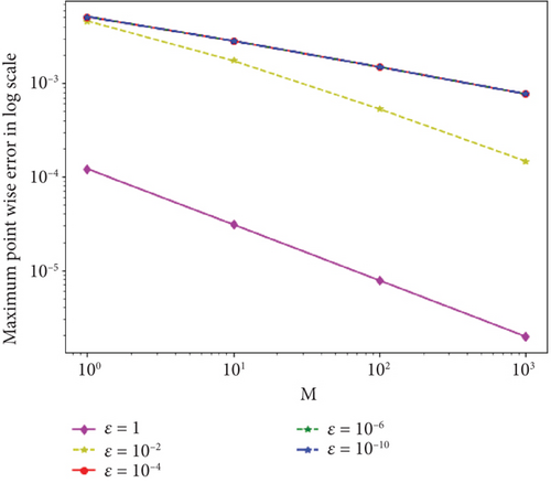
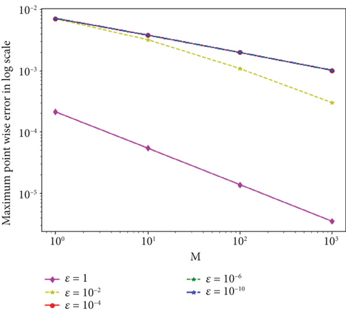
For different values of ε, N and M with a fixed α = 0.6, the maximum pointwise error (E^M,N) and the convergence rate (R^M,N) for Example 1 and Example 2 are shown in Tables 1 and 2, respectively. Similarly, for different values of α, N and M with a fixed ε = 10⁻¹⁰, the maximum pointwise error (E^M,N) and the convergence rate (R^M,N) for for both examples are given in Tables 3 and 4. From the results shown in Tables 1, 2, 3, and 4, it is observed that the maximum pointwise error decreases as the mesh size increases in both directions, which guarantees the ε-uniform convergence of the proposed method. In addition, from the last rows of Tables 1 and 2, it is observed that the present scheme is almost first-order convergent, which is in agreement with the theoretical prediction as shown in Theorem 2. The computed results in Tables 5 and 6 show the comparison of the maximum pointwise error for Examples 1 and 2 of the proposed scheme with the results in [39] for different values of α and a fixed ε. From the numerical results shown in these tables, one clearly observed that the proposed scheme is more accurate than the methods presented in [39].

Table 1. Maximum pointwise error and convergence rate of Example 1 for α = 0.6 with different values of ε.

ε = 10^−k ↓ /(M, N)⟶	(20,16)	(40,32)	(80,64)	(160,128)
k = 0	1.2109 × 10⁻⁴	3.0801 × 10⁻⁵	7.7815 × 10⁻⁶	1.9582 × 10⁻⁶
k = 0	1.9963	1.9988	1.9998	1.9999
k = 2	4.6027 × 10⁻³	1.7283 × 10⁻³	5.2719 × 10⁻⁴	1.4619 × 10⁻⁴
k = 2	1.4391	1.7297	1.8614	1.9625
k = 4	5.1056 × 10⁻³	2.8148 × 10⁻³	1.4828 × 10⁻³	7.6295 × 10⁻⁴
k = 4	0.8902	0.9456	0.9726	0.9863
k = 6	5.1056 × 10⁻³	2.8148 × 10⁻³	1.4828 × 10⁻³	7.6295 × 10⁻⁴
k = 6	0.8902	0.9456	0.9726	0.9863
k = 8	5.1056 × 10⁻³	2.8148 × 10⁻³	1.4828 × 10⁻³	7.6295 × 10⁻⁴
k = 8	0.8902	0.9456	0.9726	0.9863
k = 10	5.1056 × 10⁻³	2.8148 × 10⁻³	1.4828 × 10⁻³	7.6295 × 10⁻⁴
k = 10	0.8902	0.9456	0.9726	0.9863
k = 15	5.1056 × 10⁻³	2.8148 × 10⁻³	1.4828 × 10⁻³	7.6295 × 10⁻⁴
k = 15	0.8902	0.9456	0.9726	0.9863
k = 20	5.1056 × 10⁻³	2.8148 × 10⁻³	1.4828 × 10⁻³	7.6295 × 10⁻⁴
k = 20	0.8902	0.9456	0.9726	0.9863
E^M,N	5.1056 × 10⁻³	2.8148 × 10⁻³	1.4828 × 10⁻³	7.6295 × 10⁻⁴
R^M,N	0.8902	0.9456	0.9726	0.9863

Table 2. Maximum pointwise error and convergence rate of Example 2 for α = 0.6 with different values of ε.

ε = 10^−k ↓ /(M, N)⟶	(20,16)	(40,32)	(80,64)	(160,128)
k = 0	2.1230 × 10⁻⁴	5.4155 × 10⁻⁵	1.3726 × 10⁻⁵	3.4612 × 10⁻⁶
k = 0	1.9991	1.9989	1.9999	1.9999
k = 2	7.0014 × 10⁻³	3.2028 × 10⁻³	1.0799 × 10⁻³	2.9984 × 10⁻⁴
k = 2	1.1786	1.6015	1.8706	1.9650
k = 4	7.1030 × 10⁻³	3.7983 × 10⁻³	1.9731 × 10⁻³	1.0092 × 10⁻³
k = 4	0.9538	0.9785	0.9895	0.9948
k = 6	7.1030 × 10⁻³	3.7983 × 10⁻³	1.9731 × 10⁻³	1.0092 × 10⁻³
k = 6	0.9538	0.9785	0.9895	0.9948
k = 8	7.1030 × 10⁻³	3.7983 × 10⁻³	1.9731 × 10⁻³	1.0092 × 10⁻³
k = 8	0.9538	0.9785	0.9895	0.9948
k = 10	7.1030 × 10⁻³	3.7983 × 10⁻³	1.9731 × 10⁻³	1.0092 × 10⁻³
k = 10	0.9538	0.9785	0.9895	0.9948
k = 15	7.1030 × 10⁻³	3.7983 × 10⁻³	1.9731 × 10⁻³	1.0092 × 10⁻³
k = 15	0.9538	0.9785	0.9895	0.9948
k = 20	7.1030 × 10⁻³	3.7983 × 10⁻³	1.9731 × 10⁻³	1.0092 × 10⁻³
k = 20	0.9538	0.9785	0.9895	0.9948
E^M,N	7.1030 × 10⁻³	3.7983 × 10⁻³	1.9731 × 10⁻³	1.0092 × 10⁻³
R^M,N	0.9538	0.9785	0.9895	0.9948

Table 3. Maximum pointwise error and convergence rate of Example 1 for ε = 10⁻¹⁰ with different values of α.

α ↓ /(M, N)⟶	(20,16)	(40,32)	(80,64)	(160,128)
α = 0.2	4.7541 × 10⁻³	2.5979 × 10⁻³	1.3678 × 10⁻³	7.0623 × 10⁻⁴
α = 0.2	0.8988	0.9495	0.9748	0.9873
α = 0.4	4.9551 × 10⁻³	2.7301 × 10⁻³	1.4420 × 10⁻³	7.4470 × 10⁻⁴
α = 0.4	0.8938	0.9471	0.9735	0.9866
α = 0.6	5.1056 × 10⁻³	2.8148 × 10⁻³	1.4828 × 10⁻³	7.6295 × 10⁻⁴
α = 0.6	0.8902	0.9456	0.9726	0.9863
α = 0.8	5.2144 × 10⁻³	2.8668 × 10⁻³	1.5043 × 10⁻³	7.7126 × 10⁻⁴
α = 0.8	0.8875	0.9448	0.9722	0.9862

Table 4. Maximum pointwise error and convergence rate of Example 2 for ε = 10⁻¹⁰ with different values of α.

α ↓ /(M, N)⟶	(20,16)	(40,32)	(80,64)	(160,128)
α = 0.2	6.3266 × 10⁻³	3.5718 × 10⁻³	1.8937 × 10⁻³	9.6561 × 10⁻⁴
α = 0.2	0.7903	0.8837	0.9415	0.9703
α = 0.4	6.7404 × 10⁻³	3.6148 × 10⁻³	1.8884 × 10⁻³	9.7163 × 10⁻⁴
α = 0.4	0.9491	0.9762	0.9889	0.9946
α = 0.6	7.1030 × 10⁻³	3.7983 × 10⁻³	1.9731 × 10⁻³	1.0092 × 10⁻³
α = 0.6	0.9538	0.9785	0.9895	0.9948
α = 0.8	7.3881 × 10⁻³	3.9148 × 10⁻³	2.0203 × 10⁻³	1.0272 × 10⁻³
α = 0.8	0.9566	0.9781	0.9897	0.9950

Table 5. Comparison of maximum pointwise error of Example 1 for ε = 2⁻¹⁰ with different values of α.

α ↓ /(M, N)⟶	(16,20)	(32,40)	(64,80)	(128,160)
Present scheme
α = 0.25	5.8292 × 10⁻³	3.2563 × 10⁻³	1.7312 × 10⁻³	8.8143 × 10⁻⁴
α = 0.5	6.0987 × 10⁻³	3.4265 × 10⁻³	1.8221 × 10⁻³	9.2528 × 10⁻⁴
α = 0.75	6.2706 × 10⁻³	3.5156 × 10⁻³	1.8617 × 10⁻³	9.4114 × 10⁻⁴
Result in [39]
α = 0.25	1.1726 × 10⁻²	6.3654 × 10⁻²	3.3194 × 10⁻²	1.6943 × 10⁻³
α = 0.5	1.2246 × 10⁻²	6.6457 × 10⁻³	3.4625 × 10⁻³	1.7661 × 10⁻³
α = 0.75	1.3012 × 10⁻²	7.0750 × 10⁻³	3.6857 × 10⁻³	1.8785 × 10⁻³

Table 6. Comparison of maximum pointwise error of Example 2 for ε = 2⁻¹⁰ with different values of α.

α ↓ /(M, N)⟶	(16,20)	(32,40)	(64,80)	(128,160)
Present scheme
α = 0.25	7.9518 × 10⁻³	4.2875 × 10⁻³	2.2446 × 10⁻³	1.1561 × 10⁻³
α = 0.5	8.6536 × 10⁻³	4.6519 × 10⁻³	2.4276 × 10⁻³	1.2447 × 10⁻³
α = 0.75	9.1252 × 10⁻³	4.8630 × 10⁻³	2.5156 × 10⁻³	1.2798 × 10⁻³
Result in [36]
α = 0.25	2.3562 × 10⁻²	1.0942 × 10⁻²	5.2006 × 10⁻³	2.5142 × 10⁻³
α = 0.5	2.4877 × 10⁻²	1.1527 × 10⁻²	5.4771 × 10⁻³	2.6471 × 10⁻³
α = 0.75	2.6875 × 10⁻²	1.2479 × 10⁻²	5.9366 × 10⁻³	2.8698 × 10⁻³

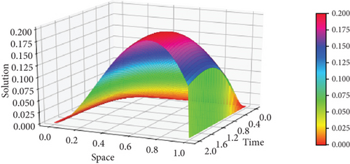
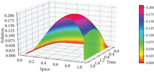
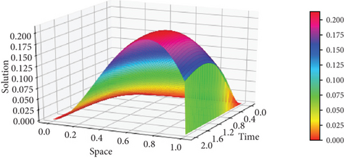
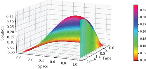
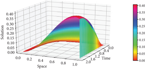
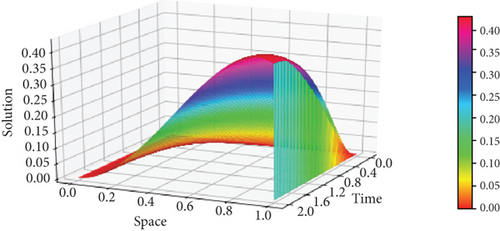
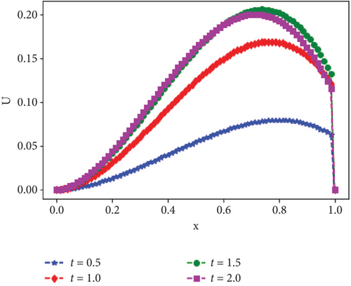
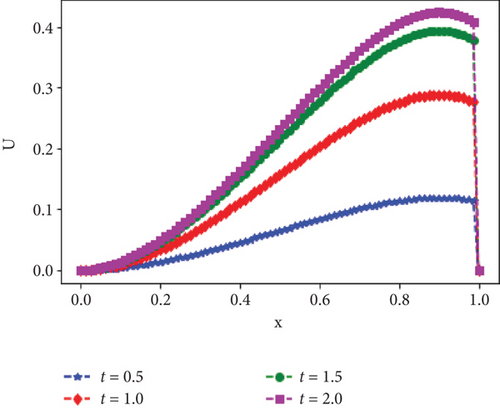
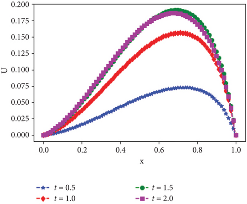
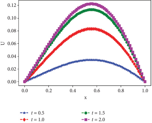
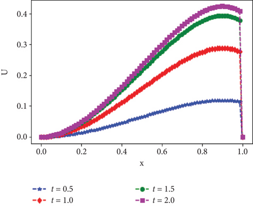
Moreover, the surface plots of the numerical solutions of Example 1 and Example 2 are shown in Figures 1 and 2, respectively, and confirm that the boundary layer is located on the right side of the rectangular domain, that is, along x = 1. In addition, these figures visualize the effects of ε and α on the boundary layer. As the perturbation parameter ε⟶0, the solution behaves more abruptly, and when the fractional order α of the Caputo fractional derivative tends to 1, the resulting figure as shown in Figures 1 and 2 approaches the classical derivative. In other words, as α approaches 1, the Caputo fractional derivative converges to the ordinary derivative. The line plots of Example 1 and Example 2 for α = 0.4 and α = 0.6 with ε = 10⁻¹⁰ are given in Figures 3 and 4, respectively. Similarly, to visualize the effects of ε on the width of the boundary layer for Example 1 and Example 2, the line plots are given in Figures 5 and 6, respectively. The maximum pointwise errors for the solutions for Example 1 and Example 2 are also plotted on a log–log scale in Figure 7. In this figure, one can observe the parameter uniform convergence of the proposed method.

Details are in the caption following the image — **Figure 1 (a) α = 0.2**
Open in figure viewer PowerPoint

3D plot of Example 1 for ε = 10⁻¹⁰, M = 80, and N = 64.

6. Conclusion

This article presents a parameter uniformly convergent numerical approach to solve one-dimensional time-fractional SPPDEs with large time delay exhibiting a regular right boundary layer. The domain is discretized with a uniform mesh in both time and space variables. The numerical scheme comprises the L1 scheme to approximate the time-fractional derivative and NSFDM together with simple upwind scheme to approximate the space derivatives. The stability and uniform convergence of the scheme is analyzed. It is shown that the proposed numerical scheme is parameter-uniform convergent and has a rate of convergence O((Δt)^2−α + Δx). To validate the applicability of the proposed scheme, two test examples are presented and the numerical results support the theoretical predictions. The advantage of the proposed numerical method is that it is easy for implementation and it gives more accurate results. To demonstrate the efficiency of the proposed numerical scheme, comparisons have been made with the results of one pioneering work available in the literature.

In our future research, the authors will further develop a higher-order uniformly convergent numerical scheme to solve time-fractional SPPDEs with time delay that improves the accuracy of the proposed numerical scheme in this article.

Conflicts of Interest

The authors declare no conflicts of interest.

Funding

The authors received no specific funding for this work.

Acknowledgments

The authors are very grateful to the reviewers for carefully reading the manuscript and for their comments and suggestions that have improved the paper very much.

Open Research

Data Availability Statement

Data are contained within the article.

References

1 Singh S., Kumar D., and Ramos H., An efficient parameter uniform spline-based technique for singularly perturbed weakly coupled reaction-diffusion systems, Journal of Applied Analysis & Computation. (2023) 13, no. 4, 2203–2228, https://doi.org/10.11948/20220446.
10.11948/20220446
Google Scholar
2 Mbroh N. A. and Munyakazi J. B., A fitted operator finite difference method of lines for singularly perturbed parabolic convection–diffusion problems, Mathematics and Computers in Simulation. (2019) 165, 156–171, https://doi.org/10.1016/j.matcom.2019.03.007, 2-s2.0-85063640339.
10.1016/j.matcom.2019.03.007
Web of Science® Google Scholar
3 Mickens R. E., Advances in the Applications of Nonstandard Finite Difference Schemes, 2005, World Scientific, https://doi.org/10.1142/5884, 2-s2.0-84967622871.
10.1142/5884
Google Scholar
4 Gülsu M., Öztürk Y., and Anapali A., Numerical solution the fractional Bagley–Torvik equation arising in fluid mechanics, International Journal of Computer Mathematics. (2017) 94, no. 1, 173–184, https://doi.org/10.1080/00207160.2015.1099633, 2-s2.0-84945152000.
10.1080/00207160.2015.1099633
Google Scholar
5 Fitt A., Goodwin A., Ronaldson K., and Wakeham W., A fractional differential equation for a mems viscometer used in the oil industry, Journal of Computational and Applied Mathematics. (2009) 229, no. 2, 373–381, https://doi.org/10.1016/j.cam.2008.04.018, 2-s2.0-67349206588.
10.1016/j.cam.2008.04.018
Web of Science® Google Scholar
6 Benson D. A., Wheatcraft S. W., and Meerschaert M. M., Application of a fractional advection-dispersion equation, Water Resources Research. (2000) 36, no. 6, 1403–1412, https://doi.org/10.1029/2000WR900031, 2-s2.0-0034032484.
10.1029/2000WR900031
Web of Science® Google Scholar
7 Cartea A. and del Castillo-Negrete D., Fractional diffusion models of option prices in markets with jumps, Physica A: Statistical Mechanics and its Applications. (2007) 374, no. 2, 749–763, https://doi.org/10.1016/j.physa.2006.08.071, 2-s2.0-33751093078.
10.1016/j.physa.2006.08.071
Web of Science® Google Scholar
8 Deng Z. Q., De Lima J. L., de Lima M. I., and Singh V. P., A fractional dispersion model for overland solute transport, Water Resources Research. (2006) 42, no. 3, https://doi.org/10.1029/2005WR004146, 2-s2.0-33646517721.
10.1029/2005WR004146
Google Scholar
9 Kilbas A. A., Srivastava H. M., and Trujillo J. J., Theory and Applications of Fractional Differential Equations, 2006, 204, Elsevier.
10.1016/S0304-0208(06)80001-0
Google Scholar
10 Choudhary R., Singh S., and Kumar D., A second-order numerical scheme for the time-fractional partial differential equations with a time delay, Computational and Applied Mathematics. (2022) 41, no. 3, 1–28, https://doi.org/10.1007/s40314-022-01810-9.
10.1007/s40314-022-01810-9
Web of Science® Google Scholar
11 Liu X., Abbas M., Yang H., Qin X., and Nazir T., Existence of chaos for partial difference equations via tangent and cotangent functions, Advances in Difference Equations. (2021) 2021, no. 1, 22, https://doi.org/10.1186/s13662-020-03162-2.
10.1186/s13662-020-03162-2
Google Scholar
12 Atangana A., On the singular perturbations for fractional differential equation, The Scientific World Journal. (2014) 2014, no. 1, 9, 752371, https://doi.org/10.1155/2014/752371, 2-s2.0-84896322966.
10.1155/2014/752371
PubMed Google Scholar
13 Chen C. M., Liu F., Turner I., and Anh V., A Fourier method for the fractional diffusion equation describing sub-diffusion, Journal of Computational Physics. (2007) 227, no. 2, 886–897, https://doi.org/10.1016/j.jcp.2007.05.012, 2-s2.0-36149001420.
10.1016/j.jcp.2007.05.012
Web of Science® Google Scholar
14 Birajdar G. A., Numerical solution of time fractional Navier-Stokes equation by discrete Adomian decomposition method, Nonlinear Engineering. (2014) 3, no. 1, 21–26, https://doi.org/10.1515/nleng-2012-0004.
10.1515/nleng-2012-0004
Google Scholar
15 Daraghmeh A., Qatanani N., and Saadeh A., Numerical solution of fractional differential equations, Applied Mathematics. (2020) 11, no. 11, 1100–1115, https://doi.org/10.4236/am.2020.1111074.
10.4236/am.2020.1111074
Google Scholar
16 Odibat Z. and Momani S., Application of variational iteration method to nonlinear differential equations of fractional order, International Journal of Nonlinear Sciences and Numerical Simulation. (2006) 7, no. 1, 27–34, https://doi.org/10.1515/IJNSNS.2006.7.1.27, 2-s2.0-30344464250.
10.1515/IJNSNS.2006.7.1.27
Web of Science® Google Scholar
17 Odibat Z., Momani S., and Erturk V. S., Generalized differential transform method: application to differential equations of fractional order, Applied Mathematics and Computation. (2008) 197, no. 2, 467–477, https://doi.org/10.1016/j.amc.2007.07.068, 2-s2.0-39449122795.
10.1016/j.amc.2007.07.068
Web of Science® Google Scholar
18 Karatay I., Kale N., and Bayramoglu S., A new difference scheme for time fractional heat equations based on the Crank-Nicholson method, Fractional Calculus and Applied Analysis. (2013) 16, no. 4, 892–910, https://doi.org/10.2478/s13540-013-0055-2, 2-s2.0-84888116422.
10.2478/s13540-013-0055-2
Web of Science® Google Scholar
19 Su L., Wang W., and Yang Z., Finite difference approximations for the fractional advection–diffusion equation, Physics Letters A. (2009) 373, no. 48, 4405–4408, https://doi.org/10.1016/j.physleta.2009.10.004, 2-s2.0-74249113616.
10.1016/j.physleta.2009.10.004
CAS Web of Science® Google Scholar
20 Song L. and Wang W., Solution of the fractional black-scholes option pricing model by finite difference method, Abstract and Applied Analysis. (2013) 2013, 10, https://doi.org/10.1155/2013/194286, 2-s2.0-84880168354, 194286.
10.1155/2013/194286
Google Scholar
21 Zhao Z., Zheng Y., and Guo P., A Galerkin finite element scheme for time–space fractional diffusion equation, International Journal of Computer Mathematics. (2016) 93, no. 7, 1212–1225, https://doi.org/10.1080/00207160.2015.1044986, 2-s2.0-84930397361.
10.1080/00207160.2015.1044986
Google Scholar
22 Li Y. and Zhao W., Haar wavelet operational matrix of fractional order integration and its applications in solving the fractional order differential equations, Applied Mathematics and Computation. (2010) 216, no. 8, 2276–2285, https://doi.org/10.1016/j.amc.2010.03.063, 2-s2.0-77953135236.
10.1016/j.amc.2010.03.063
Web of Science® Google Scholar
23 Saw V. and Kumar S., The Chebyshev collocation method for a class of time fractional convection-diffusion equation with variable coefficients, Mathematical Methods in the Applied Sciences. (2021) 44, no. 8, 6666–6678, https://doi.org/10.1002/mma.7215.
10.1002/mma.7215
Web of Science® Google Scholar
24 Rihan F. A., Computational methods for delay parabolic and time-fractional partial differential equations, Numerical Methods for Partial Differential Equations. (2010) 26, no. 6, 1556–1571, https://doi.org/10.1002/num.20504, 2-s2.0-78650109836.
10.1002/num.20504
Web of Science® Google Scholar
25 Ansari A., Bakr S., and Shishkin G., A parameter-robust finite difference method for singularly perturbed delay parabolic partial differential equations, Journal of Computational and Applied Mathematics. (2007) 205, no. 1, 552–566, https://doi.org/10.1016/j.cam.2006.05.032, 2-s2.0-34247535463.
10.1016/j.cam.2006.05.032
Web of Science® Google Scholar
26 Das A. and Natesan S., Second-order uniformly convergent numerical method for singularly perturbed delay parabolic partial differential equations, International Journal of Computer Mathematics. (2018) 95, no. 3, 490–510, https://doi.org/10.1080/00207160.2017.1290439, 2-s2.0-85014557906.
10.1080/00207160.2017.1290439
Web of Science® Google Scholar
27 Govindarao L. and Mohapatra J., A second order numerical method for singularly perturbed delay parabolic partial differential equation, Engineering Computations. (2019) 36, no. 2, 420–444, https://doi.org/10.1108/EC-08-2018-0337, 2-s2.0-85058347474.
10.1108/EC-08-2018-0337
Google Scholar
28 Kumar D. and Kumari P., A parameter-uniform numerical scheme for the parabolic singularly perturbed initial boundary value problems with large time delay, Journal of Applied Mathematics and Computing. (2019) 59, no. 1-2, 179–206, https://doi.org/10.1007/s12190-018-1174-z, 2-s2.0-85041893391.
10.1007/s12190-018-1174-z
Web of Science® Google Scholar
29 Podila P. C. and Kumar K., A new stable finite difference scheme and its convergence for time-delayed singularly perturbed parabolic PDEs, Computational and Applied Mathematics. (2020) 39, no. 3, 1–16, https://doi.org/10.1007/s40314-020-01170-2.
10.1007/s40314-020-01170-2
Google Scholar
30 Govindarao L. and Mohapatra J., Numerical analysis and simulation of delay parabolic partial differential equation involving a small parameter, Engineering Computations. (2019) 37, no. 1, 289–312, https://doi.org/10.1108/EC-03-2019-0115, 2-s2.0-85071654741.
10.1108/EC-03-2019-0115
Google Scholar
31 Tiruneh A. A., Derese G. A., and Tefera D. M., A nonstandard fitted operator method for singularly perturbed parabolic reaction-diffusion problems with a large time delay, International Journal of Mathematics and Mathematical Sciences. (2022) 2022, 11, https://doi.org/10.1155/2022/5625049, 5625049.
10.1155/2022/5625049
Google Scholar
32 Lalu M. and Phaneendra K., A numerical approach for singularly perturbed nonlinear delay differential equations using a trigonometric spline, Computational and Mathematical Methods. (2022) 2022, 10, https://doi.org/10.1155/2022/8338661, 8338661.
10.1155/2022/8338661
Google Scholar
33 Prasad E. S., Omkar R., and Phaneendra K., Fitted parameter exponential spline method for singularly perturbed delay differential equations with a large delay, Computational and Mathematical Methods. (2022) 2022, 11, https://doi.org/10.1155/2022/9291834, 9291834.
10.1155/2022/9291834
Google Scholar
34 Kumar K., Podila P. C., Das P., and Ramos H., A graded mesh refinement approach for boundary layer originated singularly perturbed time-delayed parabolic convection diffusion problems, Mathematical Methods in the Applied Sciences. (2021) 44, no. 16, 12332–12350, https://doi.org/10.1002/mma.7358.
10.1002/mma.7358
Web of Science® Google Scholar
35 Sahoo S. K. and Gupta V., A robust uniformly convergent finite difference scheme for the time-fractional singularly perturbed convection-diffusion problem, Computers & Mathematics with Applications. (2023) 137, 126–146, https://doi.org/10.1016/j.camwa.2023.02.016.
10.1016/j.camwa.2023.02.016
Web of Science® Google Scholar
36 Sahoo S. K., Gupta V., and Dubey S., A robust higher-order finite difference technique for a time-fractional singularly perturbed problem, Mathematics and Computers in Simulation. (2024) 215, 43–68, https://doi.org/10.1016/j.matcom.2023.08.013.
10.1016/j.matcom.2023.08.013
Google Scholar
37 Kumie H. G., Tiruneh A. A., and Derese G. A., Crank-Nicolson method for solving time-fractional singularly perturbed delay partial differential equations, Research in Mathematics. (2024) 11, no. 1, 1–15, https://doi.org/10.1080/27684830.2023.2293373.
10.1080/27684830.2023.2293373
Google Scholar
38 Aniley W. T. and Duressa G. F., Nonstandard finite difference method for time-fractional singularly perturbed convection–diffusion problems with a delay in time, Results in Applied Mathematics. (2024) 21, article 100432, https://doi.org/10.1016/j.rinam.2024.100432.
10.1016/j.rinam.2024.100432
Google Scholar
39 Kumar K., Podila P. C., and Vigo-Aguiar J., Numerical solution of time-fractional singularly perturbed convection–diffusion problems with a delay in time, Mathematical Methods in the Applied Sciences. (2021) 44, no. 4, 3080–3097, https://doi.org/10.1002/mma.6477.
10.1002/mma.6477
Web of Science® Google Scholar
40 Patidar K. C., High order fitted operator numerical method for self-adjoint singular perturbation problems, Applied Mathematics and Computation. (2005) 171, no. 1, 547–566, https://doi.org/10.1016/j.amc.2005.01.069, 2-s2.0-28444453616.
10.1016/j.amc.2005.01.069
Web of Science® Google Scholar
41 Al-Refai M., On the fractional derivatives at extrema points, Electronic Journal of Qualitative Theory of Differential Equations. (2012) 2012, no. 55, 1–5, https://doi.org/10.14232/ejqtde.2012.1.55.
10.14232/ejqtde.2012.1.55
Google Scholar
42 Kellogg R. B. and Tsan A., Analysis of some difference approximations for a singular perturbation problem without turning points, Mathematics of Computation. (1978) 32, no. 144, 1025–1039, https://doi.org/10.1090/S0025-5718-1978-0483484-9, 2-s2.0-84966216257.
10.1090/S0025-5718-1978-0483484-9
Web of Science® Google Scholar
43 Turuna D. A., Woldaregay M. M., and Duressa G. F., Uniformly convergent numerical method for singularly perturbed convection-diffusion problems, Kyungpook Mathematical Journal. (2020) 60, no. 3, 629–645, https://doi.org/10.1090/S0025-5718-1978-0483484-9, 2-s2.0-84966216257.
10.1090/S0025-5718-1978-0483484-9
Google Scholar
44 Doolan E. P., Miller J. J., and Schilders W. H., Uniform Numerical Methods for Problems With Initial and Boundary Layers, 1980, Boole Press.
Google Scholar

Citing Literature

All articles

Parameter-Uniform Convergent Numerical Approach for Time-Fractional Singularly Perturbed Partial Differential Equations With Large Time Delay

Abstract

1. Introduction

2. Formulation of the Continuous Problem

2.1. Properties of the Continuous Problem

3. Numerical Scheme

3.1. Time Discretization

3.2. Spatial Discretization

4. Convergence Analysis of the Fully Discrete Scheme

5. Numerical Examples

6. Conclusion

Conflicts of Interest

Funding

Acknowledgments

Open Research

Data Availability Statement

References

Citing Literature

Figures

References

Information

About Wiley Online Library

Help & Support

Opportunities

Connect with Wiley

Parameter-Uniform Convergent Numerical Approach for Time-Fractional Singularly Perturbed Partial Differential Equations With Large Time Delay

Abstract

1. Introduction

2. Formulation of the Continuous Problem

2.1. Properties of the Continuous Problem

3. Numerical Scheme

3.1. Time Discretization

3.2. Spatial Discretization

4. Convergence Analysis of the Fully Discrete Scheme

5. Numerical Examples

6. Conclusion

Conflicts of Interest

Funding

Acknowledgments

Open Research

Data Availability Statement

References

Citing Literature

Figures

References

Related

Information