Volume 2024, Issue 1 3680383

Research Article

Open Access

The Sequential Conformable Langevin-Type Differential Equations and Their Applications to the RLC Electric Circuit Problems

M. Aydin

orcid.org/0000-0003-0132-9636

Department of Medical Services and Techniques, Muradiye Vocational School, Van Yuzuncu Yil University, Van, Turkey yyu.edu.tr

Search for more papers by this author

N. I. Mahmudov,

Corresponding Author

N. I. Mahmudov

[email protected]

orcid.org/0000-0003-3943-1732

Department of Mathematics, Eastern Mediterranean University, Famagusta 99628, Turkish Republic of Northern Cyprus, Mersin 10, Turkey emu.edu.tr

Research Center of Econophysics, Azerbaijan State University of Economics (UNEC), Istiqlaliyyat St. 6, Baku 1001, Azerbaijan unec.edu.az

Search for more papers by this author

M. Aydin,

M. Aydin

orcid.org/0000-0003-0132-9636

Department of Medical Services and Techniques, Muradiye Vocational School, Van Yuzuncu Yil University, Van, Turkey yyu.edu.tr

Search for more papers by this author

N. I. Mahmudov,

Corresponding Author

N. I. Mahmudov

[email protected]

orcid.org/0000-0003-3943-1732

Department of Mathematics, Eastern Mediterranean University, Famagusta 99628, Turkish Republic of Northern Cyprus, Mersin 10, Turkey emu.edu.tr

Research Center of Econophysics, Azerbaijan State University of Economics (UNEC), Istiqlaliyyat St. 6, Baku 1001, Azerbaijan unec.edu.az

Search for more papers by this author

First published: 21 May 2024

https://doi.org/10.1155/2024/3680383

Citations: 3

Academic Editor: Waleed Adel

Share a link

Email
Wechat
Bluesky

Abstract

In this paper, the sequential conformable Langevin-type differential equation is studied. A representation of a solution consisting of the newly defined conformable bivariate Mittag-Leffler function to its nonhomogeneous and linear version is obtained via the conformable Laplace transforms’ technique. Also, existence and uniqueness of a global solution to its nonlinear version are obtained. The existence and uniqueness of solutions are shown with respect to the weighted norm defined in compliance with (conformable) exponential function. The concept of the Ulam–Hyers stability of solutions is debated based on the fixed-point approach. The LRC electrical circuits are presented as an application to the described system. Simulated and numerical instances are offered to instantiate our abstract findings.

1. Introduction

Although fractional calculus which can be seen as an extension of traditional calculus is as old as classical calculus, it has become the center of attention in the last decades because fractional differential equations consisting of fractional derivatives which are the most significant subject of fractional calculus express the real-world problem more appropriately in the most of fields such as diffusion [1], engineering [2], tuberculosis (TB) models [3], physics [4], and mathematical physics [5]. Many researchers such as Riemann and Caputo have tried to define what fractional derivatives are since the foundation of the fractional derivative was laid in 1695. In these definitions, there are some drawbacks; for example, some of them do not guarantee that the fractional derivatives of a constant are equal to zero and almost all of them do not fulfill the well-known chain rule, as in the integer order derivatives. In 2014, the conformable derivative given in [6], which is a novel definition and fulfills most of the mentioned above setbacks, was launched. In fact, this new definition is an extension of the traditional derivative of a function. We have observed that fractional derivative becomes an important part of scientific world and is mainly used in the field of health such as the growth of COVID-19 [7, 8], power-law modeling of coronavirus [9], modeling coronavirus disease [10], the Ebola epidemic disease [11], the hantavirus of the European moles [12], and in some mathematical models [13–17]. For more information about conformable derivatives, we advise the readers to look at the works [18–20] and the references therein.

Brownian motion describes the motion or progress of physical (substantial) phenomena in fluctuating environments. In the early 1900s, a full description of Brownian motion was given by Paul Langevin who was the French physicist and known as the ancestor of the Langevin equations. The fractional Langevin equation (FLE) is a stochastic differential equation that describes the motion of a particle undergoing random fluctuations in a medium with memory effects. Unlike the classical Langevin equation, which assumes that the random forces acting on a particle are white noise (independent and identically distributed), the FLE incorporates fractional Brownian motion or fractional Gaussian noise, which exhibits long-range correlations. The standard Langevin equation for the motion of a particle is given by

( )

where m is the particle mass, γ is the friction coefficient, x(t) is the particle’s position, k_B is the Boltzmann constant, T is the temperature, and ξ(t) is Gaussian white noise with zero mean and unit variance.

The FLE introduces a fractional derivative in time to model the memory effects in the system. The fractional derivative is usually described using the Riemann–Liouville fractional derivative or the Caputo fractional derivative. The study of fractional Langevin dynamics is relevant in various fields, including physics, biology, and finance, where systems with long-range memory and non-Markovian behavior are observed. Analytical solutions for the FLE are challenging to obtain, and numerical methods are often employed for simulations and analysis. Key applications of FLEs include the following: biological systems: modeling subdiffusion and superdiffusion in biological systems, such as cell movement, protein dynamics, and other intracellular processes; financial markets: describing the behavior of financial assets with long-range dependencies and memory effects; polymer physics: capturing the anomalous diffusion behavior of polymer chains in complex environments; geophysics: modeling the transport of contaminants in heterogeneous geological formations; and material science: understanding the diffusion of particles in disordered materials.

Many researchers make efforts to generalize the classical Langevin equations; for example, fractional Langevin-type equations are the production of these efforts. Even that is enough to show that the traditional Langevin equations fall short or remain incapable of describing some of today’s sophisticated problems in complicated fluctuating media. Recent works have provided more precise representations of existence and uniqueness results for both initial value problems (IVPs) and boundary value problems associated with nonlinear FLEs. Baghani and Nieto [21] demonstrated the existence and uniqueness of solutions through the application of Banach’s contractive mapping principle, while Yu, Deng, and Luo [22] explored the same aspects using Leray–Schauder’s alternative to derive analytical solutions for nonlinear FLEs. Additionally, Yu, Deng, and Luo [22] introduced sufficient conditions for a unique solution using Banach’s fixed-point theorem. Baghani [23] specifically addressed the existence and uniqueness of analytical solutions for the IVP in Langevin-type differential equations. Wei, Li, and Chea [24] tackled the existence and uniqueness problem for the IVP of fractional differential equations involving Riemann–Liouville-type fractional sequential derivatives, employing an iteration technique. In [25], the authors established sufficient criteria for the existence of solutions for nonlinear Langevin equation involving conformable operators of different orders and equipped with integral boundary conditions. Wei, Li, and Chea [24] investigated the theorem regarding the existence and uniqueness of solutions and explored the practical application of Langevin differential equations with fractional orders in various intriguing scenarios, particularly focusing on their relevance to electrical circuits. Some studies have been done on the nonlinear fractional Langevin-type equations which were introduced and researched in many aspects such as existence and uniqueness [26, 27], solutions [28], interpretation of the fractional oscillator process [29], solvability [30], and stability [31]. To the best of our knowledge, there is no study on IVPs governed by the nonlinear sequential conformable Langevin-type differential equations (SCFLDEs).

To fill this gap, we consider the following nonlinear SCFLDEs:

(1)

where

represents the conformable derivative of order (1/2) < α ≤ 1, μ and λ are real numbers, and f is a continuous disturbance from [0, T] × ℝ to ℝ. Here,

for n = 1, 2, ⋯.

Our efforts are aimed at obtaining a representation of solutions to inhomogeneous linear sequential conformable equations of the Langevin type. This is achieved through the use of the consistent conformable Laplace transform, which is recognized as a highly efficient and powerful tool for solving various differential systems. In addition, having a formula for representing the solution of a linear sequential conformable equation, we study the qualitative properties of nonlinear sequential conformable equations of Langevin type, such as uniqueness, existence, and stability.

The article presents several innovations:

•
We introduce a novel two-dimensional conformable Mittag-Leffler function.
•
A representation of the linear system associated with the nonlinear system is provided.
•
The existence and uniqueness of a solution to our system are investigated, with a focus on its stability.
•
LRC circuits are reformulated as an application to tailor our system.

This paper is organized as follows. We give a short brief about fractional derivatives and Langevin equations and describe our system in Section 1. We share necessary and available tools and concepts in the literature in Section 2. We introduce the conformable bivariate Mittag-Leffler function and look for a representation of a solution to our system in Section 3. We debate about the existence and uniqueness of a solution to our system and its stability in Section 4. We reformulate the LRC circuits as an application to adapt our system in Section 5. We offer numerical and simulated examples to verify our results in Section 6. We summarize all we discover and express some of the open problems in Section 7.

2. Preliminaries

In this section, we remind necessary tools to enable the readers to understand the coming proofs and statements more clearly.

Let a, b ∈ ℝ which is the set of all real numbers. For −∞<a < b < ∞, J = [a, b] is the interval of ℝ, and let

be the Banach space of vector-value continuous functions from J⟶ℝ given with the infinity norm

( )

for a norm ‖.‖ on ℝ.

Definition 1 (see [6].)The following fractional expression

( )

is named as the conformable derivative of order α with the lower bound of a function f : [0, ∞)⟶ℝ. Additionally, if f(.) is differentiable and

exists,

Lemma 1 (see [18].)The conformable derivative of order 0 < α ≤ 1 of a function f : [0, ∞)⟶ℝ exists if it is differentiable at x, and also, holds.

Definition 2 (see [6].)The conformable derivative of order 0 < α ≤ 1 with the lower bound of a function f : [0, ∞)⟶ℝ is given by

( )

Definition 3 (see [20].)The conformable derivative of order n < α ≤ n + 1 with the lower bound of a function f : [0, ∞)⟶ℝ is given by

( )

Proposition 1 (see [20].)Assume that f : [0, ∞)⟶ℝ and 0 < α, β ≤ 1 such that 1 < α + β ≤ 2. Then,

(2)

We give a special case of Proposition 1 in the following corollary.

Corollary 1. Assume that f : [0, ∞)⟶ℝ and 1 < 2α ≤ 2. Then,

( )

For α = β in Equation (2), the following is obtained:

( )

Lemma 2 (see [20].)Assume that f : [0, ∞)⟶ℝ and α ∈ (0, 1]. Then, we have

( )

Definition 4 (see [20].)For every t ≥ 0, the exponential function in the conformable sense is defined as follows:

( )

where d ∈ ℝ, 0 < α ≤ 1.

Definition 5 (see [32].)If a function f satisfies ‖f(t)‖ ≤ ME_α(d, t) for all sufficiently large t, where 0 < α ≤ 1, M and d are positive real numbers; then, f is exponentially bounded in the conformable sense.

Definition 6 (see [32].)The Laplace integral transform of order 0 < α ≤ 1 starting from zero of f in the conformable sense is defined as follows:

( )

where the function f : [0, ∞)⟶ℝ.

From the reference [33], we also know that

(3)

where F_α(t), which is the conformable Laplace transform of f(t), exists.

Theorem 1 (see [33].)Let f(t) be piecewise continuous on t ≥ 0 and have a conformable exponential order at infinity with |f(t)| ≤ ME(a, t) for t ≥ C. Then, the conformable Laplace transform exists for s > a.

Theorem 2 (see [34].)Suppose f(t), , ,…, are continuous and is piecewise continuous on any interval [0, T]. Assume further that f(t), ,…, have a conformable exponential order at infinity. Then, exists and

( )

where

for n = 1, 2, ⋯.

For n = 1, one has

(4)

And also, for n = 2,

(5)

Theorem 3 (see [35].)Assume that f, g : [0, ∞)⟶ℝ and 0 < α ≤ 1. The convolution in the conformable sense of f and g is defined by

( )

provided that the conformable Laplace transforms of both f and g exist for s > 0.

The gamma function for conformable integral is defined as follows:

( )

Proposition 2 (see [36].)The gamma function Γ_α(β) in the conformable sense holds the following identities:

1.
Γ_α(β + 1) = (β + α − 1)Γ_α(β)
2.
Γ_α(β) = α^{(β + α − 1)/α}Γ((β + α − 1)/α)
3.
Γ_α(1) = α

where Γ is the well-known gamma function.

Theorem 4 (see [36].)For p > 0, 0 < α ≤ 1, the conformable Laplace transforms of 1, t, and t^p are equal to

Theorem 5 (see [20].)Let r be both nonnegative and continuous on an interval [a, b] and σ and d be nonnegative constants such that

( )

Then, for all t ∈ [a, b],

( )

Definition 7. The system (1) is said to be Ulam–Hyers stable if for every ε > 0 and every solution y ∈ C([0, T], ℝ) of inequality,

(6)

Then, there exists a solution ν ∈ C([0, T], ℝ) of the system (1) and a real number ς > 0 such that

(7)

Remark 1. A function y ∈ C¹([0, T], ℝⁿ) is a solution of the inequality Equation (6) if and only if there exists a function ρ ∈ C([0, T], ℝⁿ) for every ε > 0, such that

•
‖ρ(t)‖ < ε
•

From Section 3 on, we share our novel contributions.

3. A Representation of Solutions of the Linear System

In this section which is the principle and longest part of the current paper, we spend our efforts to get a representation of solutions to nonhomogeneous linear SCFLDEs via the conformable Laplace integral transformation which is the most useful and powerful tool to solve many differential systems.

So as not to get bogged down in the details of the upcoming proofs, we need to make some preparations by offering lemmas which are valuable all by themselves.

Lemma 3. The following expressions hold true.

( )

where λ, μ ∈ ℝ, s > 0.

Proof 1. We prove the first one by using the binomial series. Based on |λ/s| < 1, one has

( )

In the light of the first item and geometric series with |μ/(s² − λs)| < 1 and |λ/s| < 1, one gets

( )

Definition 8. The conformable bivariate Mittag-Leffler function E_α,β,γ(u, v): [0, ∞)⟶ℝ is defined as follows:

( )

where α, β, γ > 0 and u, v ∈ ℝ.

Lemma 4. We have the following equalities, for λ, μ ∈ ℝ, (1/2) < α ≤ 1, and s > 0,

( )

Proof 2. Under the choices of λ, μ ∈ ℝ, 0 < α ≤ 1, and s > 0, we take the former into consideration

( )

We use Equation (3), Theorem 3, and the former one to show the trueness of the latter one:

( )

The representation of solutions to the system (1) is stated in the sequent theorem.

Theorem 6. Assume that the conformable Laplace transform of , , ν(t), and f(t) exists. The following

( )

is a representation of a solution to the system (1) with f(t, ν(t)) = f(t).

Proof 3. Applying the conformable Laplace integral transformation to the system (1), we get

( )

Implementing Equations (4) and (5) to the above equation, we get

( )

We employ common factor brackets to rearrange the upper equation

( )

Taking the conformable Laplace inverse transform on both sides in the below equation with the help of Equation (3), we acquire

( )

With the aid of Lemma 4, the desired result can be obtained as follows:

( )

Lemma 5. The following expression holds true.

( )

Proof 4. Using the substitution u = (t^α/α) − (s^α/α), one can get

( )

Lemma 6. The conformable Langevin differential Equation (1) is equivalent to the following integral equation:

(8)

Proof 5. Applying the conformable integral to the Langevin differential Equation (1) twice via Lemma 2, one can easily get

( )

Again repeat the same action for the just-above equality, one can get

( )

Corollary 1 provides what we want as the following equality:

( )

Theorem 7. Suppose that Equation (1) has a unique continuous solution ν(t) on [0, T]. If f and for 0 < α ≤ 1 are conformable exponentially bounded on [0, T], then the conformable Laplace transformations of ν(t) and for 1 < 2α ≤ 2 exist.

Proof 6. Lemma 6 expresses that each solution of Equation (1) is also a solution of Equation (8) and vice versa. We simplify Equation (8) as noted below.

( )

Due to the fact that f(t) is conformable exponentially bounded, we have

(9)

and since ν(t) and f(t) are also continuous, they are bounded on the interval [0, T], that is,

(10)

Setting

( )

For t ≥ K, we have

( )

When inequalities (10) are used in the just-above inequality, one can get

( )

We multiply both sides of the inequality by E_α(−δ, t) and use the inequalities E_α(−δ, t) ≤ E_α(−δ, K) for t ≥ K and E_α(−δ, t) ≤ E_α(−δ, s) for t ≥ s to acquire

( )

Due to Equation (9) and Lemma 5, we easily get

( )

If we denote

( )

then by Lemma 5, we get the following outcome:

( )

This means that ν is conformable exponentially bounded on [0, T]. Since f and for 0 < α ≤ 1 are also conformable exponentially bounded on [0, T] from the statement of the theorem, for 1 < 2α ≤ 2 is also conformable exponentially bounded on [0, T] because it is a linear combination of expressions that are conformable exponentially bounded. This is the desired result.

4. Existence and Uniqueness Results and System Stability

In the current section, we first discuss whether a solution to the nonlinear sequential conformable Langevin-type differential system (1) is unique in addition to whether it exists. In the sequel, we debate the concept of stability analysis in terms of solutions to the system (1) based on the fixed-point approach.

Theorem 8. The estimation which is given below always holds true.

( )

d is -1 or 0, α > 0, and μ, λ, and t are real numbers.

Proof 7. Under the restrictions on the parameter, we get

( )

By using the relationship between the conformable gamma function and the well-known gamma function, one gets

( )

and also by properties of the gamma function, one acquires

( )

If one combines these facts, the below inequality is acquired:

( )

If we replace t with t^α/α, we get the estimation expressed in the following corollary.

Corollary 2. Let α > 0 and let μ, λ, and t be real numbers.

( )

Theorem 9. Assume that f : [0, T] × ℝ⟶ℝ is so continuous that it satisfies the Lipschitz condition with the Lipschitz constant L_f, that is,

( )

The nonlinear sequential conformable Langevin system (1) has a unique solution on C²([0, T], ℝ).

Proof 8. As a norm on C²([0, T], ℝ), we define the following function:

( )

Since the well-known space (C²([0, T], ℝ), ‖.‖_∞) is complete with respect to ‖.‖_∞ and ‖.‖_∞ and ‖.‖_w are equivalent, C²([0, T], ℝ) is complete with respect to ‖.‖_w. Now, we define

( )

One can rewrite the above equation as follows with the help of Theorem 3:

( )

Consider the following expression for ν, u ∈ ℝ,

( )

By exploiting Corollary 2, Lemma 5, and the Lipschitz property of f, one gets

( )

and by taking the norm ‖.‖_w on the left-hand side, one acquires

( )

It is possible to choose sufficiently large w > 0 such that

( )

This means that is a contraction. By Banach’s fixed-point theorem, has a unique fixed point. Based on this, one understands that a representation of solutions to the system (1) is both existent and unique on C²([0, T], ℝ).

Theorem 10. Assume that f is a Lipschitzian function with respect to the second component. Then, the system (1) is stable in the Ulam–Hyers sense.

Proof 9. Let η ∈ C²([0, T], ℝ) that fulfills the inequality (6), and let u ∈ C²([0, T], ℝ) that is the unique solution of the system (1) with u₀ = η₀, u₁ = η₁. By employing the rule of and Remark 1, one can have

( )

and also has

for each t ∈ [0, T] due to its uniqueness. One can make an estimation:

( )

Now, everything is ready to estimate |u(t) − η(t)|:

( )

which offers

( )

From the just-above inequality, one can easily get the desired result:

( )

which concludes the proof.

5. An Application to the LRC Circuits

In the present section, we share an LRC electrical circuit that has widespread applications such as the tuning process of television sets, radio receivers, communication systems, and signal processing, to exemplify our theoretical findings, especially offered by Theorem 6.

Second-order nonhomogeneous linear ordinary differential equations arise in the study of electrical circuits after the application of Kirchhoff’s law [37, 38].

Suppose that I(t) is the current in the LRC series electrical circuit where circuit elements L, R, and C stand for the inductance, resistance, and capacitance, respectively. The voltage drops are of inductor, resistor, and capacitor corresponding to L(dI/dt), RI, and Q/C, respectively, that is,

(11)

which have been obtained from experimental data, where Q is the charge of the capacitor and

( )

Our goal is to model this LRC electrical circuit with an IVP so that we can determine the current and charge in the circuit.

For convenience, the units of inductance (L), resistance (R), capacitance (C), charge (Q), and current (I) as electrical quantities are henry (H), ohm (Ω), farad (F), coulomb (C), and ampere (A).

Kirchhoff’s law expressing that the sum of the voltage drops across the circuit elements is equivalent to the voltage E(t) impressed on the circuit is the physical principle to model the differential equation of the LRC circuit. According to Kirchhoff’s law, one knows that

( )

From Equation (11), one can obtain the following differential equations:

( )

By using the following facts that

( )

we get

( )

An IVP including ordinary derivatives is expressed as follows:

(12)

for the charge Q(t) and Q^′(t) = I(t).

We can remodel the IVP for the sequential Langevin-type differential equation by replacing ordinary derivatives with fractional derivatives 0 < α ≤ 1, 1 < 2α ≤ 2. In this context, the desired IVP can be reformulated as noted below:

(13)

where

( )

From Theorem 6, we get an explicit solution of the IVP (13) as stated below:

( )

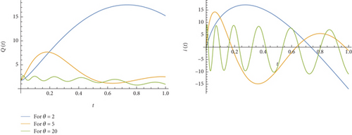
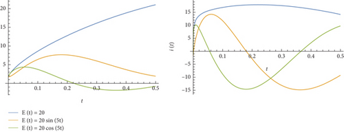
For all simulations, we select the common parameters α = 0.55, L = 10, R = 20, C = 1/15, Q₀ = 1, and Q₁ = 0.6. The graphs of the charge Q and current I for E(t) = 20 together with the common parameters are placed in Figure 1. The charges Q and currents I for distinct frequencies θ = 2, 5, 20 in E(t) = 20sin(θt) are plotted in Figure 2. For E(t) = 20, E(t) = 20sin(2t), and E(t) = 20cos(2t), the charges Q and currents I are drawn in Figure 3.

Remark 2. As shown in Figure 2, the wavelengths of the currents decrease as frequency values increase. It can be read from Figure 3 that E(t) and I(t) are of similar characteristic properties, their amplitudes may be different, and there may also be a phase shift in charge differences.

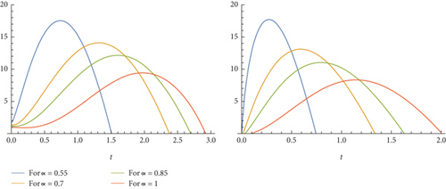
Remark 3. Under the choices of L = 10, R = 20, C = 1/15, Q₀ = 1, Q₁ = 0, 6, and E(t) = 20sin(2t), the charges Q and currents I corresponding to each of α = 0.55, α = 0.7, α = 0.85, and α = 1 are drawn in Figure 4. It is observed that the maximum current values of the system decrease while α values in the system increase.

Details are in the caption following the image — **Figure 1**
Open in figure viewer PowerPoint

Graphs of the charge Q and current I in an LRC circuit.

6. Examples

In this section, we exemplify Theorems 6, 9, and 10.

Example 1. We consider the following linear SCFLDEs:

(14)

It is clear that the system (14) becomes the system (1) with its parameters assigned by certain values. Based on Theorem 6, one gets an explicit solution in a closed form to the system (14) as noted below:

( )

whose graph can be found in Figure 5.

Example 2. We consider the following nonlinear SCFLDEs:

(15)

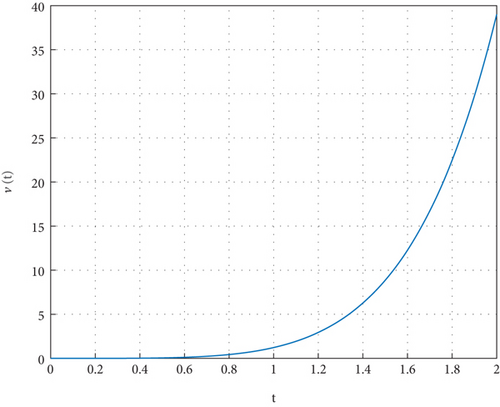
It is clear that the system (15) becomes the system (1) with its parameters assigned by certain values. Based on Theorem 6, one gets the global solution in a closed form to the system (15) as noted below:

( )

One can easily show that the disturbance function f(t) = tan⁻¹(ν(t))/(2 + t⁶) is a Lipschitzian function with respect to the second component as shown below

( )

for ν, u ∈ ℝ. With the Lipschitz constant L_f = 1/2, the condition stated in Theorems 9 and 10 is held. According to Theorems 9 and 10, the system (15) which is the Ulam–Hyers stable has a unique solution on [0, 8].

7. Conclusion

We introduce the SCFLDE. With the help of the conformable bivariate Mittag-Leffler function, an exact analytical solution to linear SCFLDE is obtained through the conformable Laplace transforms. A representation of it is extended to a global solution to the nonlinear SCFLDE. In the sequel, we show that the nonlinear SCFLDE which is stable has a unique solution. We give a detailed application of the LRC circuits and simulated and numerical instances to instantiate our abstract findings. The coming research could be devoted to the notions of asymptotic stability, finite time stability, exponential stability, and Lyapunov-type stability. Another possible study is to ask whether it is approximately controllable or controllable through iterative learning. As another possible study, the system in the case of the general fractional orders may be reconsidered. One can investigate all mentioned above things about the SCFLDE with variable coefficients obtained by replacing constant coefficients with variable coefficients.

Conflicts of Interest

The authors declare no conflicts of interest.

Author Contributions

N. I. Mahmudov carried out the concept and design of the article and helped to draft the manuscript. M. Aydin performed analysis and interpretation of data for this paper, conceived the study, participated in its design and coordination, and drafted the manuscript. All authors read and approved the final manuscript.

Funding

The authors received no specific funding for this work.

Open Research

Data Availability Statement

No underlying data was collected or produced in this study.

References

1 Obembe A. D., Hossain M. E., and Abu-Khamsin S. A., Variable-order derivative time fractional diffusion model for heterogeneous porous media, Journal of Petroleum Science and Engineering. (2017) 152, 391–405, https://doi.org/10.1016/j.petrol.2017.03.015, 2-s2.0-85015420080.
10.1016/j.petrol.2017.03.015
CAS Web of Science® Google Scholar
2 Coimbra C. F. M., Mechanics with variable-order differential operators, Annals of Physics. (2003) 515, no. 11-12, 692–703, https://doi.org/10.1002/andp.200351511-1203.
10.1002/andp.200351511-1203
Google Scholar
3 Sweilam N. H. and Al-Mekhlafi S. M., Numerical study for multi-strain tuberculosis (TB) model of variable-order fractional derivatives, Journal of Advanced Research. (2016) 7, no. 2, 271–283, https://doi.org/10.1016/j.jare.2015.06.004, 2-s2.0-84959452249.
10.1016/j.jare.2015.06.004
PubMed Web of Science® Google Scholar
4 Kilbas A. A., Srivastava H. M., and Trujillo J. J., Theory and Applications of Fractional Differential Equations, 2006, Elsevier Science BV, Amsterdam, The Netherlands.
10.1016/S0304-0208(06)80001-0
Google Scholar
5 Tarasov V., Handbook of Fractional Calculus with Applications, 2019, de Gruyter, Berlin, Germany.
Google Scholar
6 Khalil R., Al Horani M., Yousef A., and Sababheh M., A new definition of fractional derivative, Journal of Computational and Applied Mathematics. (2014) 264, 65–70, https://doi.org/10.1016/j.cam.2014.01.002, 2-s2.0-84893186929.
10.1016/j.cam.2014.01.002
Web of Science® Google Scholar
7 Ibrahim R. W., Altulea D., and Elobaid R. M., Dynamical system of the growth of COVID-19 with controller, Advances in Difference Equations. (2021) 2021, https://doi.org/10.1186/s13662-020-03168-w.
10.1186/s13662-020-03168-w
Web of Science® Google Scholar
8 Joshi H. and Yavuz M., Transition dynamics between a novel coinfection model of fractional-order for COVID-19 and tuberculosis via a treatment mechanism, The European Physical Journal Plus. (2023) 138, no. 5, https://doi.org/10.1140/epjp/s13360-023-04095-x, 37274455.
10.1140/epjp/s13360-023-04095-x
PubMed Web of Science® Google Scholar
9 Bonyah E., Fractional conformable and fractal-fractional power-law modeling of coronavirus, Mathematics in Engineering, Science & Aerospace (MESA). (2020) 11, 577–594.
Google Scholar
10 Abu-Shady M., The conformable fractional of mathematical model for the coronavirus disease 2019 (COVID-19 epidemic), Further Applied Mathematics. (2021) 1, no. 2, 34–42.
Google Scholar
11 Hammouch Z., Rasul R. R. Q., Ouakka A., and Elazzouzi A., Mathematical analysis and numerical simulation of the Ebola epidemic disease in the sense of conformable derivative, Chaos, Solitons & Fractals. (2022) 158, article 112006, https://doi.org/10.1016/j.chaos.2022.112006.
10.1016/j.chaos.2022.112006
Web of Science® Google Scholar
12 Allahamou A., Azroul E., Hammouch Z., and Alaoui A. L., Modeling and numerical investigation of a conformable co-infection model for describing Hantavirus of the European moles, Mathematical Methods in the Applied Sciences. (2022) 45, no. 5, 2736–2759, https://doi.org/10.1002/mma.7950.
10.1002/mma.7950
Web of Science® Google Scholar
13 Aliev F. A., Aliyev N. A., Hajiyeva N. S., and Mahmudov N. I., Some mathematical problems and their solutions for the oscillating systems with liquid dampers: a review, Applied and Computational Mathematics. (2021) 20, no. 3, 339–365.
Web of Science® Google Scholar
14 Duran S., Durur H., Yavuz M., and Yokus A., Discussion of numerical and analytical techniques for the emerging fractional order murnaghan model in materials science, Optical and Quantum Electronics. (2023) 55, no. 6, https://doi.org/10.1007/s11082-023-04838-1.
10.1007/s11082-023-04838-1
Web of Science® Google Scholar
15 Ișik E. and Dagbasi B., A compartmental fractional-order mobbing model and the determination of its parameters, Bulletin of Biomathematics. (2023) 1, no. 2, 153–176, https://doi.org/10.59292/bulletinbiomath.2023008.
10.59292/bulletinbiomath.2023008
Google Scholar
16 Yavuz M. and Sene N., Approximate solutions of the model describing fluid flow using generalized ρ-Laplace transform method and heat balance integral method, Axioms. (2020) 9, no. 4, https://doi.org/10.3390/axioms9040123.
10.3390/axioms9040123
Web of Science® Google Scholar
17 Modanlı M. and Koksal M. E., Laplace transform collocation method for telegraph equations defined by Caputo derivative, Mathematical Modelling and Numerical Simulation with Applications. (2022) 2, no. 3, 177–186, https://doi.org/10.53391/mmnsa.2022.014.
10.53391/mmnsa.2022.014
Google Scholar
18 Abdelhakim A. A. and Machado J. A. T., A critical analysis of the conformable derivative, Nonlinear Dynamics. (2019) 95, no. 4, 3063–3073, https://doi.org/10.1007/s11071-018-04741-5, 2-s2.0-85059552109.
10.1007/s11071-018-04741-5
Web of Science® Google Scholar
19 Birgani T., Chandok S., Dedovic N., and Radenovic S., A note on some recent results of the conformable fractional derivative, Advances in the Theory of Nonlinear Analysis and its Application. (2019) 3, no. 1, 11–17, https://doi.org/10.31197/atnaa.482525.
10.31197/atnaa.482525
Google Scholar
20 Abdeljawad T., On conformable fractional calculus, Journal of Computational and Applied Mathematics. (2015) 279, 57–66, https://doi.org/10.1016/j.cam.2014.10.016, 2-s2.0-84911406110.
10.1016/j.cam.2014.10.016
Web of Science® Google Scholar
21 Baghani H. and Nieto J. J., On fractional Langevin equation involving two fractional orders in different intervals, Nonlinear Analysis: Modelling and Control. (2019) 24, no. 6, 884–897, https://doi.org/10.15388/NA.2019.6.3.
10.15388/NA.2019.6.3
Web of Science® Google Scholar
22 Yu T., Deng K., and Luo M., Existence and uniqueness of solutions of initial value problems for nonlinear Langevin equation involving two fractional orders, Communications in Nonlinear Science and Numerical Simulation. (2014) 19, no. 6, 1661–1668, https://doi.org/10.1016/j.cnsns.2013.09.035, 2-s2.0-84890797227.
10.1016/j.cnsns.2013.09.035
Web of Science® Google Scholar
23 Baghani O., On fractional Langevin equation involving two fractional orders, Communications in Nonlinear Science and Numerical Simulation. (2017) 42, 675–681, https://doi.org/10.1016/j.cnsns.2016.05.023, 2-s2.0-84975883578.
10.1016/j.cnsns.2016.05.023
Web of Science® Google Scholar
24 Wei Z., Li Q., and Chea J., Initial value problems for fractional differential equations involving Riemann–Liouville sequential fractional derivative, Journal of Mathematical Analysis and Applications. (2010) 367, no. 1, 260–272, https://doi.org/10.1016/j.jmaa.2010.01.023, 2-s2.0-77049084247.
10.1016/j.jmaa.2010.01.023
Web of Science® Google Scholar
25 Ahmad B., Agarwal R. P., Alghanmi M., and Alsaedi A., Langevin equation in terms of conformable differential operators, Analele ştiinţifice ale Universităţii" Ovidius" Constanţa. Seria Matematică. (2020) 28, no. 2, 5–14, https://doi.org/10.2478/auom-2020-0016.
10.2478/auom-2020-0016
Web of Science® Google Scholar
26 Ahmad B., Nieto J. J., Alsaedi A., and El-Shahed M., A study of nonlinear langevin equation involving two fractional orders in different intervals, Nonlinear Analysis: Real World Applications. (2012) 13, no. 2, 599–606, https://doi.org/10.1016/j.nonrwa.2011.07.052, 2-s2.0-80054946851.
10.1016/j.nonrwa.2011.07.052
Web of Science® Google Scholar
27 Batiha I. M., Ouannas A., Albadarneh R., Al-Nana A. A., and Momani S., Existence and uniqueness of solutions for generalized Sturm–Liouville and Langevin equations via Caputo–Hadamard fractional-order operator, Engineering Computations. (2022) 39, no. 7, 2581–2603, https://doi.org/10.1108/EC-07-2021-0393.
10.1108/EC-07-2021-0393
Web of Science® Google Scholar
28 Lim S. C., Li M., and Teo L. P., Langevin equation with two fractional orders, Physics Letters A. (2008) 372, no. 42, 6309–6320, https://doi.org/10.1016/j.physleta.2008.08.045, 2-s2.0-52349118652.
10.1016/j.physleta.2008.08.045
CAS Web of Science® Google Scholar
29 Lim S. C. and Teo L. P., The fractional oscillator process with two indices, Journal of Physics A. (2009) 42, no. 6, 065208–066528, https://doi.org/10.1088/1751-8113/42/6/065208, 2-s2.0-64549125064.
10.1088/1751-8113/42/6/065208
Google Scholar
30 Ahmad B. and Nieto J. J., Solvability of nonlinear langevin equation involving two fractional orders with dirichlet boundary conditions, International Journal of Differential Equations. (2010) 2010, 10, https://doi.org/10.1155/2010/649486, 2-s2.0-77956906008, 649486.
10.1155/2010/649486
Google Scholar
31 Ahmadova A. and Mahmudov N. I., Langevin differential equations with general fractional orders and their applications to electric circuit theory, Journal of Computational and Applied Mathematics. (2021) 388, article 113299, https://doi.org/10.1016/j.cam.2020.113299.
10.1016/j.cam.2020.113299
Web of Science® Google Scholar
32 Silva F. S., Moreira D. M., and Moret M. A., Conformable Laplace transform of fractional differential equations, Axioms. (2018) 7, no. 3, https://doi.org/10.3390/axioms7030055, 2-s2.0-85052816342.
10.3390/axioms7030055
Google Scholar
33 Younis J., Ahmed B., AlJazzazi M., Hejaj R. A., and Aydi H., Existence and uniqueness study of the conformable Laplace transform, Journal of Mathematics. (2022) 2022, 7, https://doi.org/10.1155/2022/4554065, 4554065.
10.1155/2022/4554065
Web of Science® Google Scholar
34 Bouchenak A., Generalization of fractional Laplace transform for higher order and its application, Journal of Innovative Applied Mathematics and Computational Sciences. (2021) 1, no. 1, 79–92, https://doi.org/10.58205/jiamcs.v1i1.2.
10.58205/jiamcs.v1i1.2
Google Scholar
35 Khan N. A. and Razzaq O. A., Some properties and applications of conformable fracrional Laplace transform (CFLT), Journal of Fractional Calculus and Applications. (2018) 9, no. 1, 72–81, http://fcag-egypt.com/Journals/JFCA/.
Google Scholar
36 Sarıkaya M. Z., Akkurt A., Budak H., Yıldırım M. E., and Yıldırım H., On some special functions for conformable fractional integrals, Konuralp Journal of Mathematics. (2020) 8, no. 2, 376–383.
Google Scholar
37 Abell M. L. and Braselton J. P., Introductory Differential Equations with Boundary Value Problems, 2014, Elsevier Inc, Academic Press.
Google Scholar
38 Gill V., Modi K., and Singh Y., Analytic solutions of fractional differential equation associated with RLC electrical circuit, Journal of Statistics and Management Systems. (2018) 21, no. 4, 575–582, https://doi.org/10.1080/09720510.2018.1466966.
10.1080/09720510.2018.1466966
Google Scholar

Citing Literature

All articles

The Sequential Conformable Langevin-Type Differential Equations and Their Applications to the RLC Electric Circuit Problems

Abstract

1. Introduction

2. Preliminaries

3. A Representation of Solutions of the Linear System

4. Existence and Uniqueness Results and System Stability

5. An Application to the LRC Circuits

6. Examples

7. Conclusion

Conflicts of Interest

Author Contributions

Funding

Open Research

Data Availability Statement

References

Citing Literature

Figures

References

Information

About Wiley Online Library

Help & Support

Opportunities

Connect with Wiley

The Sequential Conformable Langevin-Type Differential Equations and Their Applications to the RLC Electric Circuit Problems

Abstract

1. Introduction

2. Preliminaries

3. A Representation of Solutions of the Linear System

4. Existence and Uniqueness Results and System Stability

5. An Application to the LRC Circuits

6. Examples

7. Conclusion

Conflicts of Interest

Author Contributions

Funding

Open Research

Data Availability Statement

References

Citing Literature

Figures

References

Related

Information