A Fault Diagnosis Method for Avionics Equipment Based on SMOTEWB-LGBM
Abstract
To tackle the common issue of imbalanced data classes in the fault diagnosis of avionics equipment, this study proposes a method that integrates the Synthetic Minority Oversampling Technique (SMOTE) with Boosting (SMOTEWB) and the Light Gradient Boosting Machine (LGBM). Initially, SMOTEWB is refined through a “successive one-vs-many balancing strategy,” which effectively addresses multiclass sample balance issues. The enhanced data is then employed for pattern recognition and classification using LGBM. Additionally, this study utilizes the Tree-structured Parzen Estimator (TPE) method and five-fold cross-validation to optimize the model’s hyperparameters, thus improving diagnostic accuracy. Experimental validation using University of California Irvine (UCI) public datasets and real-world avionics equipment fault data shows that the proposed SMOTEWB-LGBM method outperforms other common methods in handling multiclass imbalanced datasets. This new approach not only enhances fault diagnosis efficiency but also offers a potent solution for similar multiclass imbalance challenges.
1. Introduction
Fault diagnosis is a crucial technology in the Prognostics and Health Management (PHM) of avionics equipment. With the rapid advancement of integrated electronic circuit technology, module-level fault diagnosis has become increasingly significant. The primary aim of fault diagnosis is to isolate faults in the tested object to the corresponding board module. However, the electrical components in avionics equipment typically exhibit tolerances, and, due to the presence of nonlinearities and feedback loops, the fault mechanisms are complex and challenging to accurately capture with traditional mathematical models. These factors collectively heighten the difficulty of fault diagnosis, thereby increasing the demands on diagnostic techniques [1]. In response to these challenges, machine learning technology has emerged as a powerful tool for addressing fault diagnosis issues. At its core, machine learning views fault diagnosis as a pattern recognition problem, constructing diagnostic models through data-driven methods [2].
In the field of avionics equipment fault diagnosis, the issue of imbalanced data classes poses a significant challenge. Avionics equipment typically operates fault-free, resulting in limited and random fault samples, leading to characteristics of class imbalance in the data. Additionally, due to varying failure rates across different modules, there is a significant disparity in the number of samples for each fault class [3]. Traditional classifiers tend to focus on majority class samples, neglecting minority class samples and complicating the accurate recognition of these minority classes [4, 5].
To mitigate this issue, oversampling technology has become a prevalent solution. Oversampling primarily enhances the representation of minority class samples, either through simple repeated sampling or by synthesizing new minority class samples, thus boosting the classifier’s ability to distinguish these classes, and enhancing classification performance. Traditional oversampling methods, such as random oversampling, are straightforward but can lead to significant overfitting problems. To address this, Chawla et al. [6] introduced the Synthetic Minority Oversampling Technique (SMOTE) in 2002. SMOTE synthesizes new samples by performing random linear interpolation between minority class samples and their k-nearest neighbors, effectively reducing overfitting issues and pioneering new research avenues in oversampling techniques. Subsequent enhancements to SMOTE, such as Borderline-SMOTE [7], ADASYN [8], and SMOTE with Boosting (SMOTEWB) [9], have further refined the quality and classification performance of samples through various strategies. Notably, SMOTEWB integrates the AdaBoost [10] ensemble learning method, calculates the weights of different classes, and categorizes samples into good, lonely, and bad samples based on their features, employing distinct sampling strategies to effectively minimize noise introduction and enhance the quality of synthesized samples.
This study develops a new fault diagnosis method, SMOTEWB-LGBM (Light Gradient Boosting Machine) for avionics equipment by enhancing the SMOTEWB with a “successive one-vs-many balancing strategy” to effectively manage multiclass imbalanced samples. Following these improvements, the method employs the LGBM ensemble learning classifier to analyze the oversampled data. Additionally, this study utilizes the Tree-structured Parzen Estimator (TPE) algorithm and five-fold cross-validation to optimize the model’s hyperparameters, which improves diagnostic accuracy and reduces labor costs. The effectiveness and superiority of this approach have been demonstrated through applications on University of California Irvine (UCI) datasets and actual avionics equipment fault data.
The innovative aspects of this study primarily include the following enhancements: Firstly, the SMOTEWB method is refined with a successive one-versus-many balancing strategy, effectively addressing multiclass imbalances by systematically oversampling each minority class. Secondly, the integration of SMOTEWB’s oversampling with LGBM’s ensemble learning significantly boosts the accuracy and robustness of fault diagnosis. Lastly, the application of the TPE method for automatic hyperparameter optimization minimizes manual tuning, enhancing the model’s overall performance. Collectively, these advancements significantly improve the efficiency and reliability of the fault diagnosis system.
2. A Binary Oversampling Algorithm Based on SMOTEWB
As indicated in Equation (1), the SMOTE algorithm indiscriminately interpolates all minority class samples, without considering possible noise or outliers, leading to a degree of arbitrariness in sample generation.
SMOTEWB enhances the SMOTE algorithm by integrating AdaBoost to assign weights to various sample types. In each iteration, AdaBoost increases the weight of samples that were misclassified in the previous round. Samples are categorized into three types based on their characteristics, and each type undergoes a distinct sampling strategy to minimize noise introduction and reduce the impact of outliers, thus improving the quality of the synthetic samples. The specific methodology of SMOTEWB is detailed in the literature [9].
- 1.
Weight update: Each training sample is assigned a weight that reflects its likelihood of misclassification. The AdaBoost ensemble learning technique is used to increase the weight of samples that were incorrectly classified in the previous round, focusing more on these challenging samples in the subsequent round. The process is outlined below:
Here, the predicted label Fm(xi) represents the prediction result of the base classifier m, and the true label is Yi. I(Yi ≠ Fm(xi)) is an indicator function, which is one when I(Yi ≠ Fm(xi)) is true, and zero otherwise.
- 2.
Noise detection: We conduct noise detection on the dataset by establishing a noise threshold for each sample, which depends on the proportion of majority and minority class samples. Samples exceeding this threshold are classified as noise, while those below it are deemed nonnoise.
In this formula, nmaj represents the number of majority class samples, and n is the total number of samples in the training set. For a minority class sample , if its weight exceeds the noise threshold thmin, it is considered a noise sample; otherwise, it is classified as a nonnoise sample. This detection process is critical for categorizing minority class samples in the next step.
- 3.
Classification of samples: Using the results from noise detection, we dynamically determine the appropriate number of neighboring samples, denoted as k. Minority class samples are then categorized into three groups: good samples, lonely samples, and bad samples:
Good samples are nonnoise samples that include at least one majority class sample within their k-nearest neighbors.
Lonely samples are nonnoise samples that lack majority class samples within their k-nearest neighbors.
- 4.
Sample generation: To address the imbalance between minority and majority class samples, we generate new minority class samples based on a predetermined ratio.
Good samples have additional samples randomly generated using the SMOTE algorithm, which synthesizes new samples between the original sample and a majority class sample from its k-nearest neighbors.
Lonely samples are simply replicated to create new samples.
By implementing these procedures, SMOTEWB effectively tackles the issue of imbalanced binary data through strategic oversampling and the creation of synthetic samples from the minority class, thus achieving a balanced distribution of binary data.
3. Framework for Multiclass Fault Diagnosis Using the SMOTEWB-LGBM Model
3.1. Oversampling of Multiclass Samples Using the SMOTEWB
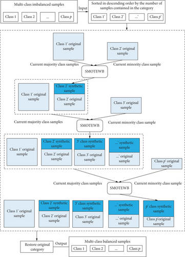
Although SMOTEWB is an effective technique for binary oversampling, it is not ideally suited for addressing imbalanced datasets with multiple classes, such as those frequently encountered in avionics equipment fault diagnosis. Specifically, datasets in this field often exhibit a significant disparity between the number of samples in the normal operating class and those in various fault classes. This variation arises due to the differing frequencies and detectability of faults across the diverse avionics modules. To tackle this challenge, our study proposes a successive one-versus-many balancing strategy that utilizes SMOTEWB to oversample the minority classes, excluding the class with the highest number of samples. This strategy aims to equalize the sample sizes across all classes, thereby enhancing the accuracy and reliability of the multiclass imbalanced dataset. The implementation process is illustrated in Figure 1.
- 1.
Rearrange the initial dataset: Organize the dataset based on the number of samples within each class and assign appropriate labels. In a dataset comprising p classes of samples, denoted as 1, 2, ⋯, p, the samples within each class are reordered in descending order by sample count, resulting in a newly arranged set of samples denoted as 1′, 2′, ⋯, p′. Notably, class 1′ has the highest number of samples, while class p′ has the fewest.
- 2.
Calculate the number of synthetic samples: Starting with the 2′-th class, generate synthetic samples in sequence until the number of samples in this class matches that of the largest class n1′, which corresponds to the 1′-th class. The required number of synthetic samples for the current class i is
- 3.
Perform successive SMOTEWB oversampling: Use the 2′-th class as the minority class and the 1′-th class as the majority class. Generate synthetic samples for the minority class using the SMOTEWB algorithm and add them to the 2′-th class. For the 3′-th class and onwards, use the i-th class as the minority class and the set of 1′, ⋯, i′ − 1 original and synthetic samples as the majority class. Generate synthetic samples for the i′-th class using the SMOTEWB algorithm and add them to the i′-th class. Stop after generating samples for the p′-th class. The final number of samples in each class will be equal to the number of samples in the 1′-th class.
- 4.
Combine all class samples: Both original and synthetic samples are combined according to their original class labels. In the final oversampled dataset, each sample retains the same class label as in the original data.
The successive one-versus-many strategy is designed to diminish the disparity in sample numbers across classes by progressively increasing the samples in each minority class. This approach considers the oversampling outcomes of previous classes, which better preserves the characteristics of the data distribution. Thanks to the robust noise handling capabilities of SMOTEWB, when combined with this strategy, it can generate higher-quality synthetic samples for minority classes, thereby achieving a more balanced distribution for multiclass imbalanced data.
By using the successive one-versus-many strategy to enhance SMOTEWB’s multiclass oversampling, we can achieve a dataset where each class has equal numbers of samples. This not only increases the quantity of training samples but also ensures a balance across different types of data, providing higher-quality training samples for subsequent LGBM pattern recognition.
3.2. LGBM Method for Fault Pattern Recognition
LGBM is a distributed system developed by Ke et al. [11] from Microsoft Research Asia in 2017. It is an enhancement of Gradient Boosting Decision Tree (GBDT) [12], known for its excellent classification capabilities [13]. After oversampling multiclass samples using the SMOTEWB model, the balanced data is fed into the LGBM model for training, enabling precise fault pattern recognition.
Here, f(x; γm) represents the weak model, βm represents the weight coefficient, and γm represents the parameters of the weak model.
Here, c is a constant value that can minimize the loss function.
Here, I(xi ∈ Rmj) is an indicator function. If xi is in the Rmj region, it results in one; otherwise, it is zero.
During the fitting process of decision trees, LGBM converts continuous floating-point eigenvalues into q integers, constructs a histogram of width q, and identifies the optimal segmentation point, substantially reducing storage requirements. The leaf-wise growth strategy, utilized in node splitting, minimizes search and splitting time while increasing accuracy by focusing on the leaves with the highest splitting gain. Furthermore, techniques such as gradient-based one-sided sampling and exclusive feature bundling in LGBM maximize data utilization and accelerate training efficiency.
3.3. Stratified K-Fold Cross-Validation
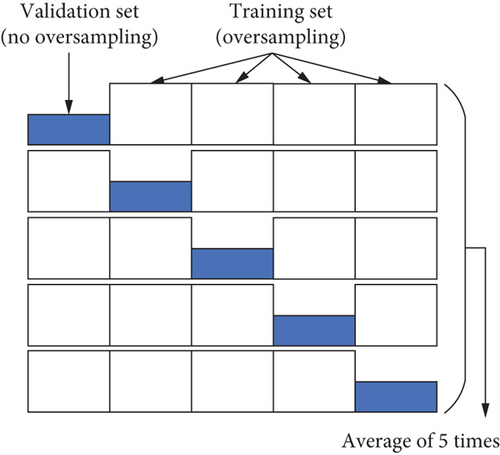
K-fold cross-validation divides the dataset into K subsets of equal size, selecting one subset to assess the model’s performance, while employing the remaining K-1 subsets for training. Given the imbalanced nature of the dataset, the stratified K-fold method is utilized to ensure that the proportion of each class in each subset mirrors that in the original dataset [14]. This approach effectively utilizes the data and mitigates the risk of overfitting. In this study, K is set to five, meaning that five-fold cross-validation is implemented. The training and validation sets are randomly divided into five parts, where each of the five subsets is oversampled using SMOTEWB to create five oversampled subsets.
The schematic diagram of five-fold cross-validation is shown in Figure 2, and to validate the effectiveness of this method, each 50% unsampled subset is used in turn as a validation set, with the corresponding four oversampled subsets serving as the training set. After completing five validation rounds, the average result of these validations represents the outcome of the cross-validation.
3.4. TPE Hyperparameter Optimization
In 2011, Bergstra et al. [15] from Harvard University introduced the TPE, a method that models the relationship between hyperparameters using a tree structure and effectively addresses multidimensional optimization challenges. With only a few iterations, TPE can achieve superior hyperparameter selection. Consequently, TPE is an optimal method for tuning the hyperparameters of the SMOTEWB-LGBM model, requiring minimal computing resources while ensuring efficient operation. This method is adaptable to different objective functions, further enhancing the quality of hyperparameter selection.
Here, x represents the observation point, which is the hyperparameter vector of the model to be optimized; y is the observation value, the outcome of the objective function (loss or evaluation function) for the given parameter x; and y∗ is a threshold, representing a specific quantile of the TPE algorithm used to divide the observations into two density functions, l(x) and g(x), with the sum ranging from zero to one. The algorithm sets y∗ based on existing observations, segregating them into two distinct density functions: l(x) is formed by those observations {x(i)} whose loss is f(x(i)) < y∗, and g(x) consists of the remaining observations. TPE employs Bayesian optimization principles to minimize ineffective search space.
Let γ = p(y < y∗), and to simplify the above formula, construct the denominator asp(x) = ∫p(x|y)p(y)dy = γl(x) + (1 − γ)g(x).
From this formula, maximizing EI involves ensuring that the probability of l(x) is high and that of g(x) is low. In each iteration, the algorithm returns the candidate hyperparameter x∗ with the highest EI value, . During the maximization process, the hyperparameter x that achieves the highest l(x) and the lowest g(x) probabilities obtains the highest EI value. The TPE algorithm uses l(x) and g(x) to generate a collection of hyperparameter samples and evaluates x by the ratio of l(x)/g(x). Each iteration returns the point with the highest EI value. Using this approach, we identify the optimal hyperparameters for the SMOTEWB-LGBM model. In optimizing these parameters, the new x is employed to construct the fault diagnosis model for the SMOTEWB-LGBM algorithm, and the observation y is obtained through training convergence. The new observation point is then compared with the original, updating the probabilistic surrogate model to select the hyperparameter x corresponding to the best result.
In this study, we utilize the microaverage F1 (Micro-F1) score from the five-fold cross-validation as the objective function for optimizing parameters through the TPE method. This method helps identify the optimal hyperparameters by maximizing the aforementioned score.
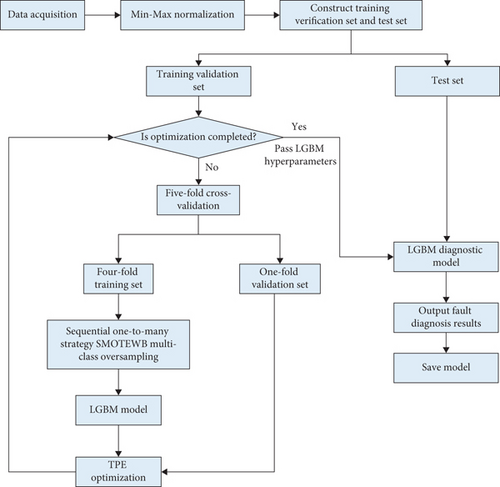
We apply the TPE algorithm to optimize hyperparameters for both SMOTEWB and LGBM simultaneously. Once optimized, the LGBM hyperparameters are then used in the LGBM model for classification diagnosis testing. Although the SMOTEWB hyperparameters do not participate directly in the testing phase, they play a crucial role during the training phase by altering the distribution of the training data through the generation of synthetic samples. This alteration aids in training a more robust LGBM classification model. The framework of this SMOTEWB-LGBM multiclass fault diagnosis is illustrated in Figure 3.
4. Evaluation Indicators and Diagnostic Process
4.1. Evaluation Indicators for Class Imbalance Problem
In traditional classification problems, classification accuracy is commonly used as a key metric to evaluate classifier performance. However, when dealing with imbalanced datasets, relying solely on classification accuracy may not accurately reflect the overall classifier performance. To overcome this limitation, this study incorporates the weighted precision (Weighted-P) as suggested in the literature [16], along with the macroaverage F1 (Macro-F1) score and the Micro-F1 score from the literature [17] as metrics to evaluate classification performance. The confusion matrix for binary classification is presented in Table 1.
| Real situation | Classification results | |
|---|---|---|
| Normal | Abnormal | |
| Normal | TP (true positive) | FN (false negative) |
| Abnormal | FP (false positive) | TN (true negative) |
To extend the F1 score to multiclass classification, two types of averaging are usually used, namely, Macro-F1 score and Micro-F1 score.
These three indicators offer different perspectives to evaluate model performance. The weighted average precision and Micro-F1 score are more sensitive to large classes, while the Macro-F1 score treats all classes as equally important. The three indicators are employed to facilitate a comprehensive analysis of algorithm performance.
4.2. Fault Diagnosis Process
The fault diagnosis process of SMOTEWB-LGBM is as follows.
Step 1. Data preprocessing including Min–Max normalization.
Step 2. Application of the SMOTEWB method with a one-to-many balancing strategy to oversample multiclass imbalanced data, equalizing the sample count across all classes.
Step 3. Pattern recognition using the LGBM ensemble learning method on the balanced data.
Step 4. Optimization of SMOTEWB and LGBM hyperparameters using the TPE algorithm and five-fold cross-validation, followed by model output.
Step 5. Determination of the mode category for new samples and identification of the fault mode.
5. Experiment and Discussion
The SMOTEWB-LGBM method proposed in this study was initially tested on datasets from the UCI and subsequently on avionics equipment for diagnostic experiments. It was also compared with other multiclassification algorithms designed for imbalanced data, such as SMOTEBoost [18], RUSBoost [19], Adacost [20], ImECOC [21], as well as LGBM, which is an ensemble learning method suitable for such data. The TPE algorithm was implemented using the Optuna [22] hyperparameter tuning framework.
The experiments were conducted in the following environment: an Intel Core i9-13900HX processor with a base frequency of 2.20 GHz and a max turbo frequency of 5.60 GHz, and 32 GB of memory. The software environment included a Windows 11 operating system and the PyCharm 2023.1 integrated development environment, using Python version 3.8.5.
5.1. Experiments on UCI Datasets
The UCI datasets, which are publicly available and commonly used to benchmark algorithm performance in machine learning, were selected to test the effectiveness of the proposed method. Six datasets with varying imbalances were used: Balance-scale, Diabetes, Dermatology, Cell-cycle, User-knowledge, and Glass. The details of these datasets are provided in Table 2.
| Dataset name | Number of samples | Number of classes | Number of features | Number of samples in each class |
|---|---|---|---|---|
| Balance-scale | 625 | 3 | 4 | 288, 49, 288 |
| Diabetes | 768 | 2 | 8 | 500, 268 |
| Dermatology | 529 | 6 | 34 | 112, 61, 72, 49, 52, 20 |
| Cell-cycle | 217 | 4 | 17 | 47, 31, 18, 121 |
| User-knowledge | 403 | 5 | 5 | 102, 129, 122, 24, 26 |
| Glass | 213 | 6 | 9 | 69, 76, 17, 13, 9, 29 |
Eighty percent of the data from each dataset were randomly selected as training samples, with the remaining 20% serving as the test set. To minimize the impact of randomness, 10 experiments were conducted on each dataset, and the results were averaged. The findings from these experiments are displayed in Table 3, with the optimal values for each indicator highlighted in bold. Corresponding graphical representations are shown in Figure 4.
| Datasets | Models | Weighted-P | Macro-F1 | Micro-F1 |
|---|---|---|---|---|
| Balance-scale | SMOTEBoost | 0.798 3 | 0.597 9 | 0.840 0 |
| RUSBoost | 0.853 4 | 0.695 1 | 0.808 0 | |
| Adacost | 0.780 4 | 0.588 8 | 0.848 0 | |
| ImECOC | 0.820 4 | 0.615 9 | 0.880 0 | |
| LGBM | 0.831 1 | 0.651 0 | 0.864 0 | |
| SMOTEWB-LGBM | 0.863 4 | 0.696 3 | 0.832 0 | |
| Diabetes | SMOTEBoost | 0.795 2 | 0.765 7 | 0.7857 |
| RUSBoost | 0.701 7 | 0.654 3 | 0.675 3 | |
| Adacost | 0.781 5 | 0.724 0 | 0.733 8 | |
| ImECOC | 0.794 9 | 0.766 7 | 0.798 7 | |
| LGBM | 0.797 8 | 0.771 7 | 0.798 7 | |
| SMOTEWB-LGBM | 0.809 8 | 0.784 2 | 0.805 2 | |
| Dermatology | SMOTEBoost | 0.928 3 | 0.935 4 | 0.918 9 |
| RUSBoost | 0.922 0 | 0.892 4 | 0.890 4 | |
| Adacost | 0.948 0 | 0.932 3 | 0.945 2 | |
| ImECOC | 0.959 2 | 0.956 3 | 0.959 4 | |
| LGBM | 0.945 5 | 0.937 6 | 0.945 2 | |
| SMOTEWB-LGBM | 0.975 6 | 0.969 2 | 0.973 0 | |
| Cell-cycle | SMOTEBoost | 0.550 2 | 0.405 6 | 0.454 5 |
| RUSBoost | 0.643 3 | 0.500 7 | 0.659 1 | |
| Adacost | 0.687 0 | 0.514 9 | 0.636 4 | |
| ImECOC | 0.637 9 | 0.470 2 | 0.659 1 | |
| LGBM | 0.502 9 | 0.618 2 | 0.636 4 | |
| SMOTEWB-LGBM | 0.834 8 | 0.593 9 | 0.727 0 | |
| User-knowledge | SMOTEBoost | 0.912 9 | 0.847 3 | 0.913 6 |
| RUSBoost | 0.695 6 | 0.497 8 | 0.691 4 | |
| Adacost | 0.654 1 | 0.394 7 | 0.567 9 | |
| ImECOC | 0.823 2 | 0.672 3 | 0.864 2 | |
| LGBM | 0.917 1 | 0.799 1 | 0.925 9 | |
| SMOTEWB-LGBM | 0.952 3 | 0.910 7 | 0.950 6 | |
| Glass | SMOTEBoost | 0.790 6 | 0.753 2 | 0.744 2 |
| RUSBoost | 0.513 0 | 0.302 6 | 0.465 1 | |
| Adacost | 0.765 9 | 0.746 1 | 0.790 8 | |
| ImECOC | 0.715 6 | 0.623 8 | 0.744 2 | |
| LGBM | 0.806 3 | 0.663 5 | 0.790 7 | |
| SMOTEWB-LGBM | 0.813 5 | 0.756 2 | 0.767 4 | |
- Numbers in bold represent the best results obtained.
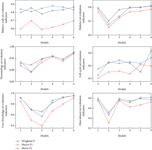
As depicted in Table 3 and Figure 4, the SMOTEWB-LGBM method achieved the highest scores across all evaluation metrics for three datasets—namely, Diabetes, Dermatology, and User-knowledge, and registered the best results in two metrics across three datasets, specifically Balance-scale, Cell-cycle, and Glass. Notably, in the Dermatology dataset, it significantly outperformed other methods. This superior performance underscores the effectiveness of combining the SMOTEWB oversampling method, which adeptly minimizes noise introduction, with the robust classification capabilities of the LGBM ensemble learning method, thus significantly enhancing the classification outcomes for multiclass imbalanced data. The success of this method across multiple datasets also demonstrates its broad applicability.
5.2. Front-End Receiver Fault Diagnosis Experiment
To assess the practical effectiveness of the SMOTEWB-LGBM diagnostic model in avionics equipment diagnosis, we applied it to the fault diagnosis of the front-end receiver in a specific type of aircraft electronic countermeasure system. Figure 5 illustrates the basic working principle of the front-end receiver. The primary function of the front-end receiver is to amplify and filter signals within its operational frequency range, convert them into video signals containing threat information, and forward these signals to both the signal processor for further processing and to the central receiver along with the low-power radio frequency unit. These radio frequency signals carry essential frequency band information pertaining to threat radars.
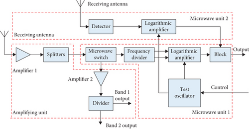
This study conducted module-level fault diagnosis on the front-end receiver. The diagnosis is distinguished between a normal mode and three fault modes based on the receiver’s functionalities. The modes are denoted as follows: normal mode (F0) and three fault modes—amplification unit module failure (F1), microwave unit 1 module failure (F2), and microwave unit 2 module failure (F3). The diagnostic parameters included 12 test measurements, representing 12-dimensional sample features: sensitivity at five frequency points, dynamic range at five frequency points, and gain at two radio frequencies.
Data collection utilized the Automatic Test System (ATS) for this type of aviation equipment, employing standard signal sources, power meters, and spectrum analyzers as specified in the factory maintenance manual. A total of 450 datasets were compiled, with 306 sets of normal samples (F0) and 63, 31, and 50 sets of fault samples for F1, F2, and F3 modes, respectively. This dataset exhibited a pronounced class imbalance.
The data were randomly divided into 80% training samples and 20% test samples. Using the Optuna hyperparameter tuning framework, the TPE algorithm, and stratified five-fold cross-validation, we simultaneously tuned the parameters of the SMOTEWB oversampling algorithm and the LGBM pattern recognition method. The four-fold training set comprised the sample post-SMOTEWB oversampling, while the validation set utilized the original data samples. SMOTEWB required tuning for two parameters, and LGBM required tuning for six parameters. Table 4 displays the optimal hyperparameters obtained through this optimization.
| Category of parameters | TPE tuning parameters | Range of parameter values | Type of parameter values | Optimal hyperparameter values |
|---|---|---|---|---|
| SMOTEWB parameters | n_iters | (30, 100) | int | 96 |
| max_depth | (5, 30) | int | 16 | |
| LGBM parameters | lambda_l1 | (0, 10) | Float | 0.1049 |
| lambda_l2 | (0, 10) | float | 0.2042 | |
| num_leaves | (3, 128) | int | 17 | |
| feature_fraction | (0.5, 1) | Float | 0.5204 | |
| bagging_fraction | (0.5, 1) | Float | 0.9395 | |
| learning_rate | (0, 1) | Float | 0.0979 | |
Figure 6 shows the distribution of class samples before and after SMOTEWB oversampling. Initially, there was a marked imbalance among the classes, with the F0 class having the most samples and the F2 class the fewest—over three times fewer than F0. This imbalance hindered optimal pattern recognition. However, after employing SMOTEWB’s successive one-versus-many strategy for oversampling, the number of samples in each class matched that of the largest class before oversampling, significantly increasing the size of the training dataset and improving the LGBM’s classification performance.
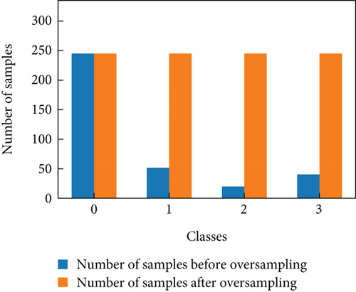
Figure 7 displays a radar chart comparing the mean values of different features for the original samples and the new samples generated by SMOTEWB oversampling. It is evident that no new samples were generated for the F0 class, which was the largest class. In contrast, new samples were created for the F1, F2, and F3 classes, with the mean values of the features for these new samples closely mirroring those of the original samples. This similarity indicates that the new samples preserved the characteristics of the original data and maintained a similar distribution, thereby more accurately representing the original minority samples.
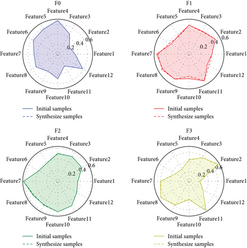
Figure 8 illustrates the trend of the multiclass logarithmic loss value from the first to the 100th iteration of the SMOTEWB-LGBM model under the optimal hyperparameter combination. The chart shows a rapid decrease in the training set loss, stabilizing at approximately 0.08284 after about 60 iterations. The test set loss converged to 0.12148. These results indicate that the default 100 iterations were adequate. The slightly higher loss on the test set compared to the training set, while still low, demonstrates that the model performed robustly on unseen data without overfitting. The minor difference between the loss values of the training and test sets confirms that the model was well-fitted, avoiding overfitting, and was effective in classifying and identifying faults.
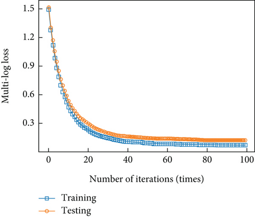
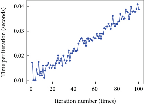
Figure 9 shows the time spent on each iteration of the model training process. The time per iteration follows a nonlinear increasing trend, suggesting that as the number of iterations grows, so does the complexity and computational load of the training process. This nonlinear increase may stem from the dynamic allocation of computational resources. Despite this rise, the overall time per iteration remains within an acceptable range, from approximately 0.01–0.041 s per iteration. The brief testing time of the model indicates its suitability for fault diagnosis in avionics equipment, fulfilling engineering requirements.
To better assess the fault diagnosis performance of the classification model under the imbalanced dataset, Figure 10 presents the model’s classification confusion matrix. The y-axis in the figure represents the actual fault labels of the data, while the x-axis shows the predicted labels.
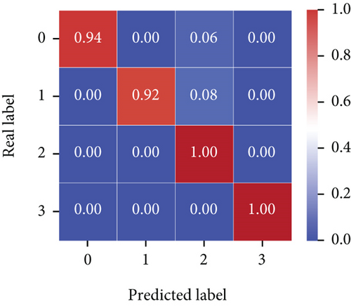
The model achieved 100% prediction accuracy for the F2 and F3 classes, and 94% and 92% classification accuracy for the F0 and F1 classes, respectively. The confusion matrix further confirms that the proposed method can effectively predict multiple classes of data under an imbalanced dataset setting, meeting the high-precision requirements for fault diagnosis of avionics equipment.
The proposed method was also experimentally compared with SMOTEBoost, RUSBoost, Adacost, ImECOC, and other methods, including LGBM. Each method was run 10 times to calculate the average value. Table 5 shows the experimental results, and Figure 11 graphically illustrates these outcomes. Additionally, the time cost of the models was compared, using default hyperparameters for each. Table 5 records the corresponding average training and testing times.
| Models | Weighted-P | Macro-F1 | Micro-F1 |
|---|---|---|---|
| SMOTEBoost | 0.923 7 | 0.892 8 | 0.918 4 |
| RUSBoost | 0.834 6 | 0.730 1 | 0.836 7 |
| Adacost | 0.857 1 | 0.794 8 | 0.816 3 |
| ImECOC | 0.865 8 | 0.781 0 | 0.836 7 |
| LGBM | 0.857 1 | 0.786 8 | 0.857 1 |
| SMOTEWB-LGBM | 0.960 5 | 0.951 0 | 0.959 2 |
- Numbers in bold represent the best results obtained.
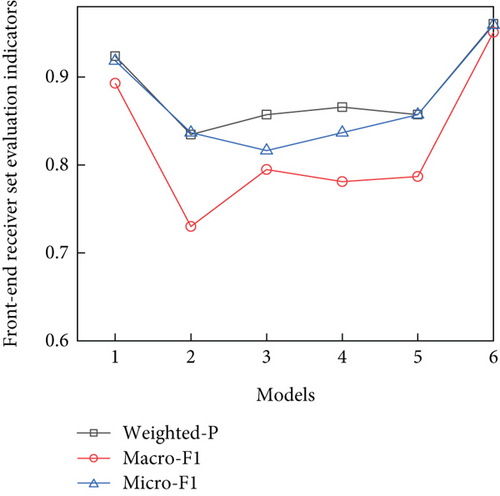
The experimental results presented in Table 5 and Figure 11 demonstrate that in the front-end receiver fault diagnosis experiment, the SMOTEWB-LGBM model outperformed other models, achieving a weighted-average precision of 96.05%, a Macro-F1 score of 95.10%, and a Micro-F1 score of 95.92%. These results indicate that the proposed method effectively meets the fault diagnosis requirement of avionics equipment.
Table 6 details the experimental outcomes of the front-end receiver under various data split ratios. It is evident that most algorithms perform optimally with an 8 : 2 data split ratio. This preference is likely due to the advantage of having a larger training set in the context of small-sample data, which provides more information for the model to learn and understand the intrinsic patterns and features of the data. This comprehensive learning typically results in better model generalization during training, leading to enhanced performance on the test set. Furthermore, the SMOTEWB-LGBM method demonstrates consistently high performance across different data split ratios, underscoring its sophistication and robustness.
| Algorithm | Weighted-P | Macro-F1 | Micro-F1 | ||||||
|---|---|---|---|---|---|---|---|---|---|
| Data segmentation ratio | 8 : 2 | 7 : 3 | 6 : 4 | 8 : 2 | 7 : 3 | 6 : 4 | 8 : 2 | 7 : 3 | 6 : 4 |
| SMOTEBoost | 0.923 7 | 0.933 5 | 0.920 6 | 0.892 8 | 0.848 5 | 0.8317 | 0.918 4 | 0.933 3 | 0.922 2 |
| RUSBoost | 0.834 6 | 0.881 0 | 0.822 3 | 0.730 1 | 0.695 8 | 0.616 2 | 0.836 7 | 0.822 2 | 0.838 9 |
| Adacost | 0.857 1 | 0.877 4 | 0.856 2 | 0.794 8 | 0.670 0 | 0.6480 | 0.816 3 | 0.800 0 | 0.783 3 |
| ImECOC | 0.865 8 | 0.820 7 | 0.819 2 | 0.781 0 | 0.569 8 | 0.5019 | 0.836 7 | 0.807 4 | 0.788 9 |
| LGBM | 0.857 1 | 0.937 1 | 0.928 2 | 0.786 8 | 0.846 2 | 0.838 6 | 0.857 1 | 0.933 3 | 0.922 2 |
| SMOTEWB-LGBM | 0.960 5 | 0.946 9 | 0.928 7 | 0.951 0 | 0.870 4 | 0.801 4 | 0.959 2 | 0.948 1 | 0.927 8 |
- Numbers in bold represent the best results obtained.
6. Conclusions
This study introduces the SMOTEWB-LGBM method, effectively addressing the challenge of multiclass imbalance in avionics equipment fault diagnosis. By integrating SMOTEWB oversampling with LGBM’s pattern recognition, the method not only improves fault diagnosis accuracy but also enhances the robustness of the system. The SMOTEWB, enhanced with a “successive one-vs-many balancing strategy,” optimizes the quality of training samples, thereby enhancing the LGBM model’s learning efficiency. Additionally, the use of the TPE method for hyperparameter optimization minimizes manual intervention, further boosting the model’s performance. Experimental results demonstrate superior performance, achieving a Weighted-P of 96.05%, a Macro-F1 score of 95.10%, and a Micro-F1 score of 95.92%, significantly outperforming existing methods like SMOTEBoost, RUSBoost, Adacost, ImECOC, and standalone LGBM.
However, the current application is limited to specific datasets. Future research will expand this method’s application to a broader range of avionics equipment and other fault diagnosis areas to verify its generalizability and effectiveness.
Conflicts of Interest
The authors declare no conflicts of interest.
Funding
This research was funded by the Mount Taishan Scholar Construction Project in Shandong Province, China, with grant number tstp20221146.
Acknowledgments
We thank the authors of smote-variants, LightGBM, and Optuna open-source code. Our code is based on their open-source code for improvement.
Open Research
Data Availability Statement
The UCI datasets used in this study are openly available in the database at https://archive.ics.uci.edu/datasets (accessed on January 1, 2024).


