International Journal of Aerospace Engineering

Volume 2024, Issue 1 2583156

Research Article

Open Access

Improved Variable Structure Interacting Multimodels for Target Trajectory Tracking and Extrapolation

Xuanming Ren,

Xuanming Ren

orcid.org/0000-0001-9685-4083

College of Civil Aviation, Nanjing University of Aeronautics and Astronautics, Nanjing 211106, China nuaa.edu.cn

Search for more papers by this author

Xinmin Tang,

Corresponding Author

Xinmin Tang

[email protected]

orcid.org/0000-0001-9573-2172

School of Transportation Science and Engineering, Civil Aviation University of China, Tianjin 300300, China cauc.edu.cn

Search for more papers by this author

Yang Zhou,

Yang Zhou

College of Civil Aviation, Nanjing University of Aeronautics and Astronautics, Nanjing 211106, China nuaa.edu.cn

Search for more papers by this author

Xiangmin Guan,

Xiangmin Guan

Key Laboratory of Civil Aviation General Aviation Operation, Civil Aviation Management Institute of China, Beijing 100102, China camic.cn

Search for more papers by this author

Xuanming Ren,

Xuanming Ren

orcid.org/0000-0001-9685-4083

College of Civil Aviation, Nanjing University of Aeronautics and Astronautics, Nanjing 211106, China nuaa.edu.cn

Search for more papers by this author

Xinmin Tang,

Corresponding Author

Xinmin Tang

[email protected]

orcid.org/0000-0001-9573-2172

School of Transportation Science and Engineering, Civil Aviation University of China, Tianjin 300300, China cauc.edu.cn

Search for more papers by this author

Yang Zhou,

Yang Zhou

College of Civil Aviation, Nanjing University of Aeronautics and Astronautics, Nanjing 211106, China nuaa.edu.cn

Search for more papers by this author

Xiangmin Guan,

Xiangmin Guan

Key Laboratory of Civil Aviation General Aviation Operation, Civil Aviation Management Institute of China, Beijing 100102, China camic.cn

Search for more papers by this author

First published: 16 May 2024

https://doi.org/10.1155/2024/2583156

Academic Editor: Chuang Liu

Share a link

Email
Wechat
Bluesky

Abstract

To improve the lengthy computation time of conventional variable structure interacting multiple model (VSIMM) algorithm and increase the precision of target prediction and extrapolation, the target state and flight intent information captured by the Automatic Dependent Surveillance-Broadcast (ADS-B) are used as the model’s prior information; combining this information with VSIMM theoretical framework, we purpose an intent variable structure interacting multiple model (INT-VSIMM) algorithm. Firstly, the motion pattern of the target in the flight phase of the flight path is decomposed, and complete sets of motion models are established. Secondly, according to the principle of directed graph switching, a model set switching method is designed, which is mainly based on “hard” switching and supplemented by “soft” switching. Finally, the INT-VSIMM algorithm is used to track the trajectory of the target aircraft, and short-term trajectory extrapolation is performed based on the target state estimation. The simulation results show that the target tracking performance computational time based on the INT-VSIMM algorithm is superior to the comparative existing methods, and the extrapolated trajectory has less error in the short term, which can satisfy the needs of conflict detection.

1. Introduction

With the rapid development of the global air transportation business, the density of aircraft in airspace has posed a challenge to the handling capacity of air controllers, which will inevitably increase the risk of accidents for aircraft in airspace [1, 2]. To this end, enabling aircrew to take on some of the conflict detection responsibilities through airborne surveillance and communication technology can effectively alleviate the workload of controllers and ensure the safety of aircraft operation.

The advancement of air surveillance technology allows the ownship to obtain flight states and intention information of the target aircraft through Automatic Dependent Surveillance-Broadcast (ADS-B) messages sent by the target aircraft [3]. Based on this information, the aircraft has the ability to track surrounding aircraft [4–6] and extrapolate their flight trajectory [7] for the near future, and providing data assistance for conflict detection. However, since the intention information of the aircraft is difficult to capture and discontinuous, the current research mainly extrapolates the flight trajectory in the near future based on the historical trajectory information of the target aircraft [8–10].

For conflict detection problems, the tracking and prediction of targets depend on the assumptions of the target motion model. Single-model estimation is a classic method for target tracking research, which is characterized by simple structure and easy implementation [11]. However, the trajectory tracking and extrapolation problem of an aircraft involves complex stochastic nonlinear mixed system state estimation, resulting in single-model estimation that is prone to cause a mismatch between aircraft’s motion pattern and predicted model. Reference [12] proposes an interactive multiple model (IMM) algorithm based on the Markov transformation coefficients. This algorithm divides the flight actions into corresponding motion modes, such as uniform motion, uniform acceleration motion, and uniform turning, so that the aircraft can match one or more corresponding motion models in each motion mode to describe aircraft motion [13, 14]. Considering that actual noise generally conforms to colored noise processes, Singer proposed the Singer model in 1970. Singer model is a global statistical model that does not require detection during target tracking; therefore, there is no time lag [15, 16]. The “current” statistical (CS) model of manoeuvring target assumes that the mean acceleration is a nonzero first-order time-dependent function, and the “current” probability density of acceleration is expressed by the modified Rayleigh distribution [17–19], which is more in line with the actual aircraft flight situation.

Owing to the utilization of a fixed model set within the IMM algorithm, to ensure a meticulous and precise depiction of the target’s motion characteristics, a substantial number of motion models need to be used to cover all possible manoeuvres of the target. As the proliferation of models escalates, model mismatch caused by model competition can lead to a decrease in tracking accuracy [20]. For this reason, reference [21] proposes a variable structure interacting multimodel (VSIMM) architecture, which builds a matching model set for each motion mode and uses the observation data to select the optimal model set to describe the current motion of the target [22–24]. Based on the VSIMM architecture, reference [25] designed a fuzzy adaptive controller and introduced a nonlinear system to adjust the self-adaptivity of parameters. Reference [26] introduces a fuzzy membership function in the CS model for adaptive regulation of target acceleration. In order to solve the problem of traditional tracking algorithm adaptive biases when tracking strong manoeuvring target, reference [27] uses a feedback network to monitor the matching degree between different models and the actual motion of the target in real-time. Although the above algorithms all utilize a posteriori information to match the optimal model set for the target’s current motion, which improves the tracking accuracy, none of them are able to use the prior information to guide the switching of the model set. Thus, the target tracking suffers from the issues of model set switching lag and model set mismatch.

In summary, this research proposes a flight intent variable structure interacting multiple model (INT-VSIMM) algorithm, aiming to enhance the situational awareness of the aircraft during the flight phase by utilizing the information of the aircraft’s flight intent. The main contributions of this research can be summarized as follows:

1.
By integrating the ADS-B data transmitted by the target aircraft, we analysed the flight status and expected flight intent of the target aircraft. On this basis, we established a complete set of models composed of four basic motion models to adapt to the motion patterns of aircraft in various flight scenarios.
2.
Based on the principle of model set switching of directed graphs, we proposed a model set switching method that mainly uses “hard” switching and supplements with “soft” switching. This method helps match the most suitable model set for the current motion of monitoring targets, thereby improving the computational accuracy and efficiency of multimodel algorithms.
3.
According to the one-step prediction result of the target’s current state, the target trajectory is extrapolated in the short term, which helps to achieve accurate and rapid conflict detection.

2. Modeling of Target Motion State

2.1. Problem Description

The airborne ADS-B out device can encode the aircraft’s status information such as longitude, latitude, altitude, speed, and heading, as well as the intention information of selecting altitude and selecting heading, and then broadcast them in the form of different types of messages. The ownship can receive and decode messages from surrounding airspace through the ADS-B in device, so as to perceive the operation state of the surrounding aircraft. As for the extrapolation of aircraft trajectory, the completeness and accuracy of captured information from other aircraft will directly affect the predicted longitude of the trajectory. In this paper, by capturing airborne position message (APM), airborne velocity message (AVM), target state, and situation message (TSSM), we obtain the target aircraft’s position information (longitude, latitude, and altitude information), speed and heading information (east-west speed, north-south speed, and climb rate information), and the flight intention information (selected altitude and selected heading information). Based on the target information, we utilize the VSIMM algorithm combined with the Kalman filter for tracking and, finally, extrapolate the short-term trajectory based on the motion trend of the target aircraft.

2.2. Kinematics Model of Ownship

The motion state of aircraft can be represented by the following discrete system state equation:

()

where Φ(t) represents state transition matrix, Γ(t) is the system noise-driven matrix, w(t) ~ N(0, Q_t) is the state equation white noise, Q(t) is the process noise covariance, and X(t) is the state vector of the system at time t.

Given that the Cartesian coordinate system causes a divergence when illustrating ADS-B height data [28], the geodetic coordinate system is chosen as the reference frame for target tracking, and writing the state variables of the target aircraft in the form of three-phase components, the target state variable X(t) can be expressed as

()

Here, α(t), β(t), and γ(t) are the component of three directions; x(t), , and are the position, velocity, and acceleration of the target aircraft in longitude direction at time t, respectively; y(t), , and are the position, velocity, and acceleration of the target aircraft in latitude direction at time t, respectively; h(t), , and are the displacement, velocity, and acceleration of the target aircraft in altitude direction at time t, respectively.

2.2.1. Constant Velocity (CV) Straight Flight

Assuming that the target moves uniformly, establish the CV motion model for the target. During the cruise phase, aircraft are mostly in a state of CV straight-line flight, so the CV model is the most basic and commonly used flight model. This model is very useful in theoretical research because it represents the basic motion state of an aircraft under ideal conditions and can serve as the basis for complex models.

The target state vector in the direction of longitude is represented as

, and w(t) is Gaussian white noise obeying [0, σ²]. For filtering and processing convenience, it is necessary to expand all motion models to the maximum dimension of the model set. Given the fourth-order state transition matrix of the turning model in the model set, we need to expand the CV_LNG model to four orders, and the expanded dimensions should be filled with 0. The discrete equation of the CV_LNG model is as follows:

()

where state vector

and

is the transition matrix,

is the system noise-driven matrix, and T is the sampling period.

Then, the target motion models along latitude direction CV_LAT and altitude direction CV_QNE are similar with CV_LNG, therefore the discrete state equation of latitude and altitude direction:

()

Here, and are the state vectors of latitude and altitude, respectively; ; .

2.2.2. Constant Acceleration Straight Flight

The constant accelerated (CA) model represents the flight state of an aircraft under the influence of constant thrust. For example, during takeoff and landing and accelerated cruising stages, aircraft usually perform constant acceleration flight. The CA model is very important for tracking and predicting the maneuverability of aircraft.

Consistent with the modeling principle of the CV model, the target’s CA motion is modeled in three directions, the discrete form of state equation:

()

Here, , , and are the state vectors, , .

2.2.3. Variable Acceleration Flight

The variable acceleration model represents the flight state of an aircraft under the influence of changing thrust. For example, in complex weather conditions or when performing special manoeuvres, such as avoiding obstacles, aircraft may perform variable acceleration flight. This model is very common in actual flight and is very useful for simulating and dealing with sudden flight conditions.

The variable acceleration motion in this article adopts the CS model, which is a first-order time-dependent model with nonzero mean acceleration, and the acceleration of the target aircraft at the next moment is based on the neighbourhood of the “current” acceleration. Despite the “current” model that can represent the manoeuvring characteristics of the target aircraft faithfully, the tracking effect is weak when the target acceleration is outside the [(4 − π/4)a_max, a_max] and [a_min, (4 − π/4)a_min] intervals. Therefore, the “current” model is not suitable for tracking less manoeuvring target aircraft.

Assuming that the motion of the target in three directions follows variable acceleration, then establish the CS model for the target based on the CS model, the discrete state equation of the CS_LNG model can be given by

()

where

, and

represent the state vector of three directions;

;

are the system input control matrixes;

;

is the estimated value of current acceleration.

2.2.4. Constant Angular Velocity Turning Flight

The constant turning (CT) model represents the aircraft turning at a constant angular velocity during horizontal flight. In actual flight, turning is a very common operation, such as in route navigation, obstacle avoidance, and tactical manoeuvres. The CT model is the basis of heading control in target tracking models.

Unlike the models based on random processes, the CT model is primarily dependent on the target’s kinematic characteristics in order to more accurately describe the target’s spatial trajectory. Considering that there are fewer cases of civil aviation manoeuvring in the vertical direction when it is cruising, this section adopts a two-dimensional model that describes horizontal motion for the CT model and uses CV_QNE, CA_QNE, and CS_QNE models for tracking in the vertical direction.

In addition, considering that the turning maneuver of target is a nonlinear motion, the longitude and latitude directions will be coupled while discretizing the state equations. Hence, we decoupled the longitude and latitude directions of the target motion state when establishing the turning model of longitude and latitude direction. The discrete state transition equation of the target aircraft can be expressed as follows:

()

where

and

are state vector,

2.2.5. Prior Information of the Model

The prior information used in this study includes the flight status information and flight intention information of the target aircraft.

ADS-B is to broadcast the precise position generated by the Global Positioning System (GPS) and the motion status stored by the airborne flight management system (FMS). Other communication terminals receive this broadcast through data links and perform decoding analysis to achieve airspace monitoring. By capturing and decoding the ADS-B APM and AVM of the target aircraft, we obtained data on the longitude, latitude, and altitude of the target aircraft, as well as the magnitude and direction of flight speed. These data reflect the current flight status information of the target aircraft. In target tracking filtering, after preprocessing the flight status information, the position, velocity, and acceleration data of the target in three directions are sequentially inserted into the observation matrix, thereby completing the update of the current target aircraft position and velocity status.

By capturing and decoding the TSSM, we can obtain FMS-selected altitude and heading data, which can serve as the flight intent information of the target aircraft, reflecting the changing trend of altitude and heading of the target in the near future. After decoding, this data is inserted into the intent matrix and used to guide the system in adopting “soft” or “hard” switching when updating the model set. The structure of message and the meaning of each field can be found in the RTCA DO-260B document [29]. The structure of the 56-bit ME field in the message is shown in Figure 1.

Details are in the caption following the image — **Figure 1 (a) Airborne position message**
Open in figure viewer PowerPoint

Message analysis result.

In this way, the target aircraft’s longitude, latitude, and altitude data can be acquired by decoding the APM and used as the observation values to update target aircraft’s current position state. Furthermore, the ground speed, heading, and vertical speed parsed through the AVM can be transformed into the speed information in three directions after projection and used as the observation values to update target aircraft’s current velocity. The observation equation in the geodetic coordinate system is

()

Here, observation matrix ; Z(t) is the observation value; v(t) is the observation noise, obeying [0, R_t], and R_t is the observation noise covariance matrix. Continuous correction of tracking errors using flight status information can effectively improve tracking accuracy. In addition to the target position, this study also added observation inputs for target velocity, which can provide a more accurate estimation of the current behaviour of the target.

Civil aircraft may send TSSM before and after scheduled waypoints or ATC-designated waypoints, especially when these points represent significant route changes or flight plan updates. This message will contain information on aircraft’s current state and flight intentions and will be broadcast at random intervals that are uniformly distributed over the range of 1.2 to 1.3 s, to ensure that other aircraft and ground control stations can understand the aircraft’s anticipated manoeuvres.

There are several fields in the TSSM message that are dedicated to representing the intent information of the target aircraft. The FMS selects altitude and heading data that reflect the expected trends in target altitude and heading and therefore serves as the flight intent of the target aircraft.

The novelty of this study is to utilize the FMS-selected altitude and selected heading data to serve as a pivotal basis for model set switching. Since the target’s flight intent information directly reflects the expected flight status of the aircraft in the near future, it is evidently faster and more accurate compared to the filtering estimation results. Using flight intent as prior information to guide model set switching will undoubtedly greatly improve inherent delays and enhance model tracking accuracy. This part of theory will be elaborated upon with meticulous detail in the ensuing section.

3. Model Set Adaptive Switching Algorithm

3.1. Model Set Based on Directed Graphs

The motion modes of target are decomposed into straight and turning flight at constant altitude, constant heading lift, and turning during lift. The above four flight modes cover all the flight manoeuvres of a civil aviation aircraft in the normal flight, and each flight mode is mathematically described by six submodels. The corresponding relationship between model set and model submodel is shown in Table 1.

Table 1. The relationship between target motion states and model submodel.

Model set U	Target motion states	Submodel m_i
U₁	Straight flight under constant altitude	CA_LNG, CV_LNG, CS_LNG, CA_LAT, CV_LAT, CS_LAT
U₂	Turning flight under constant altitude	CA_LNG, CT_LNG, CS_LNG, CA_LAT, CT_LAT, CS_LAT
U₃	Climbing/descending flight under constant heading	CA_LNG, CA_LAT, CA_QNE, CS_LNG, CS_LAT, CS_QNE
U₄	Climbing/descending under turning flight	CT_LNG, CT_LAT, CV_QNE, CS_LNG, CS_LAT, CS_QNE

The state judgment of the target adopts a combination of event-driven and model probability-driven methods, fully utilizing the prior information of the target to achieve better tracking results. Adaptively, the current model set is that switch from the previous model set to a model set that is closer to the target motion state, after the state judgment. Figure 2 depicts the directed diagram of the model set.

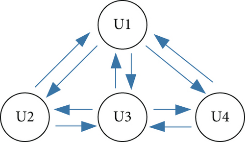
3.2. Model Set Switching Rules

The commonly used directed graph switching method is to switch the current model set to a new model set that is more suitable for the target motion state based on the system’s judgment of the target motion state at the last time. This model set switching method essentially has a certain time lag, which means that adjustments need to be made at the next moment when the target undergoes manoeuvring. This paper decodes the TSSM to extract flight intention information such as the selected altitude and heading of the target aircraft. The flight intention of an aircraft reflects its expected flight state in the near future, which is obviously more accurate compared to the predicted results of the model. Using flight intention as a prior information to guide the switching of the model set will undoubtedly enormously improve the tracking accuracy of the model and improve the fixed time lag. Thereby, this section integrates the heading and altitude flight intentions, thereupon proposes a model set switching rule based on the intent information to achieve fast and accurate model set switching.

Flight intention driven is a “hard” switching rule, and whereas it can simply and directly promote the computational efficiency and prediction accuracy of the model, the acquisition of flight intention information is not continuous in the process of tracking the target aircraft. For this reason, it is necessary to provide a “soft” switching rule as a supplementary means of model set switching. This section matches the current optimal model by calculating the likelihood probability of each model set, which can achieve “soft” switching of the model set. The principle of model set switching is shown in Figure 3.

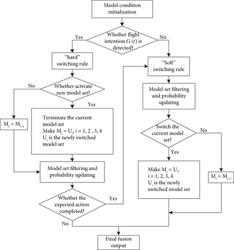
Define flight intention driven as “hard” switching. Whereas “hard” switching can simply and directly promote the computational efficiency and prediction accuracy of the model, the acquisition of flight intention information is not continuous in the process of tracking the target aircraft. For this reason, it is necessary to provide a “soft” switching rule as a supplementary means of model set switching. This section matches the current optimal model by calculating the likelihood probability of each model set, which can achieve “soft” switching of the model set.

Assuming that the system captures flight intention G(t) = [h_s(t), φ_s(t)] at time t, where h_s(t) represents the FMS-selected altitude, φ_s(t) represents the FMS-selected heading, and G(t) is the intention matrix. The “hard” switching rule based on flight intention is as follows:

()

The above “hard” switching criterion can be used to activate an individual model set, whereas the time when to terminate the model set depends on whether the target has completed the expected action as the termination condition. In other words, when the filtering result does not reach the intended set value, it indicates that the target has not completed the expected action, and then, the filtering result will be fused and output. In contrast, the filtering result has reached the intention set value, which indicates that the target has completed the expected action, and intention-based “hard” switching result will no longer be applicable; finally, the likelihood-based “soft” switching method will be used to solve the optimal model set.

The model set switching method based on the model set likelihood probability has to filter and estimate all model sets and then calculate the likelihood probability of the model set on the basis of the residual and its covariance. Taking model set U₁ as an example, after model filtering and model probability update, the maximum likelihood probability of U₁ is calculated according to residuals and covariance and compared with the maximum likelihood probability of all other model sets. Subsequently, the model set with the maximum likelihood probability is selected to be switched to the current model set and eventually output the filtering results of the optimal model set.

The advantage of this method over traditional VSIMM algorithm is that the procedure of model set switching and state estimation output can be accomplished by only one filtering, which greatly reduces the computation time. Assuming the model set likelihood probability

is the cumulative sum of the likelihood probability of each submodel

in that model set, denoted as

()

Among them, d_i(t) and S_i(t) represent the residual vector and covariance at time t, respectively, and their mathematical expressions are introduced in Section 4.

4. Tracking and Extrapolation of Target Aircraft

4.1. INT-VSIMM-Based Filtering Algorithm

The model set adaptive switching method discussed in Section 3 is incorporated into the model set sequence condition estimation to recognize the motion pattern of the target aircraft. The INT-VSIMM filtering algorithm proposed in this study consists of four parts: building a complete model set, model filtering estimation, selecting the optimal model set, and fusion output. The diagram of the algorithm is shown in Figure 4.

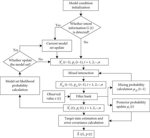
The specific steps of the INT-VSIMM algorithm are as follows.

Step 1. Model initialization

1.
Building model sets. Establish the complete model set U that is sufficient to cover all possible movements of the target aircraft.
2.
Assign transfer probabilities to submodels. Assuming that the set-model M_t contains n submodels at time t, the matrix of model transfer probabilities from model m_i to m_j(m_i ∈ M_t, m_j ∈ M_t):

()

Then, the probability of transferring from model m_i to m_j at moment t − 1 can be expressed as follows:

()

Here, u_i represents the probability that the system is model m_i at time t − 1.

Step 2. According to the “hard” switching rule introduced in Section 3, select the model set for filtering estimation.

Step 3. Model filtering estimation

1.
Filter initialization. The mixing probability from m_i to m_j:

()

Mixed state estimates for model m_j at time t − 1:

()

Mixed covariance estimation for model m_j:

()

Here, is the state estimation corresponding to the filter output of model m_i at moment t − 1, P_i(t − 1|t − 1) is the covariance matrix corresponding to the filter output of model m_i at moment t − 1, is the state input of the filter corresponding to model m_j at moment t, which is calculated by weighted summation of the state estimates output by each filter at time t − 1, and the weight is the mixed probability of each submodel to model m_j; P_0j(t − 1|t − 1) is the covariance matrix input of the filter corresponding to model m_j at time k, which is calculated by weighted summation of the covariance matrix estimates of each filter output at time t − 1; u_j|i(t − 1|t − 1) is the mixed probability that the model matches m_i at time t − 1 and m_j at time t, conditional on the information Z(t):

()

2.
Model conditional filtering.

Due to the establishment of the linear motion equation of the target in Section 2.2 and the modeling of system noise as Gaussian white noise, under the assumptions of linear system and Gaussian noise, the Kalman filter ensures that the estimated value is as close to the true value as possible by minimizing the mean square error. Of course, if the system is assumed to be nonlinear or non-Gaussian noise, using methods such as unscented Kalman is a better choice. In addition, the Kalman filter only requires one iteration to update the state estimation and has better speed and accuracy than other filtering methods in dynamic systems and short-term prediction. Finally, the Kalman filter divides state prediction and update into two steps, which makes the algorithm structure clear and facilitates the implementation of subsequent trajectory extrapolation work.

In this study, the nonlinear motion of the target is decomposed into linear motion in three directions: longitude, latitude, and altitude. In order to avoid confusing model predictions in different directions, the state input is filtered by the Kalman filter in the three directions, respectively.

One-step prediction of the state and its covariance:

()

The residual information d_j(t) and its covariance S_j(t):

()

The gain matrix of the Kalman filter is as follows:

()

Update the target state and covariance using observation data:

()

Step 4. Optimal model set switching.

1.
Maximum likelihood probability update. The updated expression for the model likelihood function Λ_j(t) is given in Equation (22) and brings the model likelihood function into Step 2 for model set switching.
2.
Model probability update

()

Here, is the probability of transferring from another model to model m_j.

3.
Select the optimal model set. Select the optimal model set according to the “soft” switching rules introduced in Section 3.

Step 5. Fusion output.

The fusion output of the filter is the weighted value of the filter estimation results after filtering each submodel in the optimal model set. The weighted state estimation and its covariance P(t|t) are as follows:

()

where

is the filter correction error, which eliminates the difference between the state filter estimate of model m_j and fusion output.

4.2. Trajectory Extrapolation Based on INT-VSIMM

According to the calculation in Section 4.2, we can track the motion state of the target aircraft at the current time, but in order to predict potential flight conflicts in advance, it is necessary to extrapolate the trajectory of the target. Since the state estimation of the target is constantly updated with observations, this section only performs short-term extrapolation of the target trajectory to provide data support for aircraft conflict detection.

As can be seen from Step 3, the one-step prediction result of the model state is only related to the state vector

, the variance

, and the model probability

, whose update is independent of the observations. Thereupon, this study employs the estimated state filtering values of a certain time model for one-step prediction, and the extrapolation results will be used as inputs for the next extrapolation calculations. Assuming that the current time is t, the probability of M_j at time t + 1 can be obtained from the full probability equation:

()

State prediction value and prediction filtering mean square matrix of INT-VSIMM:

()

Here, is the estimated value of the model m_j at time t + 1.

5. Numerical Simulation

5.1. Simulation Environment and Parameter Setting

The filtering data in this study is the ADS-B message of the aircraft with flight number CXA8830 on December 5, 2022, which is within 1400s of the climbing flight phase. Firstly, eliminate the acquired message data that was duplicated or anomalous to get 1209 trajectory points. Then, assume that the time when received the air position message is t, and the next time that received the air position message is t + 1; the duration of the discretization time step is T. Within the duration of pheromones, the decoded position and speed information is inserted into the observation matrix, and the decoded intention information is inserted into the intention matrix. According to the Nyquist sampling theorem, the sampling frequency should be at least twice the highest frequency of the signal. Therefore, this article sets T = 0.6 s.

The simulation was performed under AMD Ryzen 3 2200G processor, with 3.5 GHz main frequency and 64-bit Windows 10. The simulation results were compared with the traditional VSIMM algorithm and the IMM algorithm, and the initial parameter settings are shown in Table 2.

Table 2. Model initial parameter.

Submodel direction	Target initial state	Initial model probability	Initial model transition probability
Model set U₁
Longitude direction α
Latitude direction β
Altitude direction γ	—	—	—
Model set U₂
Longitude direction α
Latitude direction β
Altitude direction γ	—	—	—
Model set U₃
Longitude direction α
Latitude direction β
Altitude direction γ
Model set U₄
Longitude direction α
Latitude direction β
Altitude direction γ

The process noise covariance and observation noise covariance matrix of the respective models are set as follows: Γ(t) = diag(0.1², 0.1², 0.1², 0.1²) and R(t) = diag(2500, 2500, 2500,2000,2000,2000).

5.2. Simulation Results and Analysis

In the case of the simulation in this study, the prior information of the conventional VSIMM algorithm and IMM algorithms was tracked using a single observation, while the INT-VSIMM algorithm receives the intent data (select altitude 26,816 feet, select heading 87.89 degrees) additionally when the target aircraft runs up to 873 s. The comparison curves between the calculated trajectory of the three filtering algorithms and the real trajectory are shown in Figure 5.

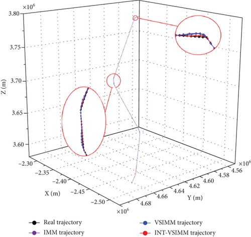
From Figure 5, it can be seen that all the three algorithms are able to realize the target tracking effectively, and among them, the conventional IMM and VSIMM algorithms do not have much difference in the tracking effect when the target changes motion pattern; however, the tracking effect of the INT-VSIMM algorithm is obviously unquestionably superior to the first two, which is closer to the real trajectory.

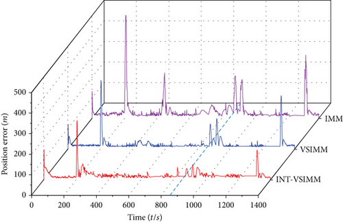
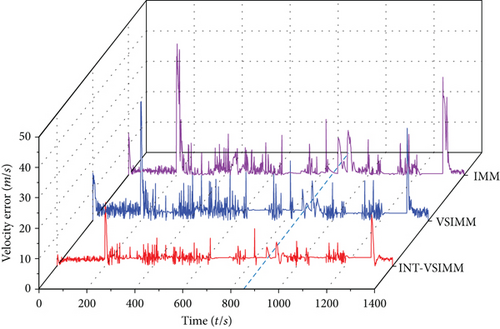
Figure 6 shows the position tracking error curves and velocity tracking error curves of the three filtering algorithms, respectively. It can be seen that when the motion mode of the target aircraft changes, the tracking error curves of the three filtering algorithms will significantly oscillate, which is basically the result from model mismatch caused by the switching delay of the model set, as well as submodel prediction confusion. The INT-VSIMM algorithm received the target’s intention data at 873 s and used it to modify the state’s heading and altitude. The maximum errors of position and velocity have been improved by 42.44% and 22.01% compared to traditional IMM algorithms and 13.54% and 8.87% compared to conventional VSIMM algorithms, respectively. The mean errors of position and velocity have been reduced by 23.57% and 25.30% compared to traditional IMM algorithms and 6.84% and 18.50% compared to conventional VSIMM algorithms, respectively. The maximum tracking error and mean error of the three filtering algorithms are shown in Table 3, and all indicators of the INT-VSIMM algorithm are optimal.

Table 3. Performance comparison of position and velocity error.

Error type	IMM algorithm	VSIMM algorithm	INT-VSIMM algorithm
Maximum position tracking error (m)	502.212	334.424	289.142
Maximum speed tracking error (m/s)	75.984	65.026	59.258
Mean position error (m)	44.692	34.157	31.822
Mean speed error (m/s)	13.077	11.985	9.768

The VSIMM algorithm based on a multimodel set architecture has multiple model sets running at any time, so it has an intrinsic increase in computation compared to fixed structure IMM filters. To address this issue, the INT-VSIMM algorithm proposed in this study reduces the filtering computation of redundant model sets by using intentional data and, in addition, optimizes the flow of the filtering algorithm, which reduces the simulation computation time by 12.08% relative to the VSIMM algorithm. The simulation time of the three filtering algorithms is shown in Table 4.

Table 4. Simulation time of trajectory tracking.

Filtering algorithm	IMM algorithm	VSIMM algorithm	INT-VSIMM algorithm
Calculative time (s)	3.522	4.900	4.308

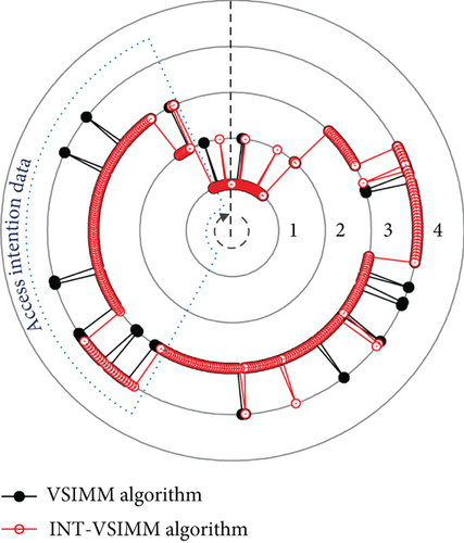
Figure 7 depicts the trend of the INT-VSIMM algorithm’s optimal model set at each instant. The black dashed line in the figure represents the starting position of the target aircraft’s motion, and the model set curve changes in a clockwise direction. From the figure, it can be seen that due to the guiding effect of intention data on model set switching, the INT-VSIMM algorithm avoids repeated model set switching during pattern recognition, thereby improving model stability and adaptability.

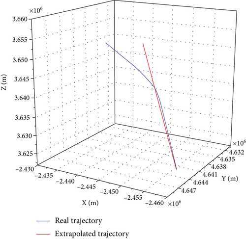
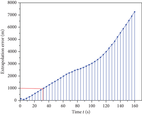
The filtered output of t = 368 s is selected as the initial state of an extrapolation of 160 s. Figures 8(a) and 6(b) show the comparison and error curves between the extrapolated trajectory and the real trajectory, respectively. It can be seen that an extrapolated trajectory can obtain better prediction results in the short term, although the extrapolation error gradually increases with the extension of extrapolation time, and the error has reached 1000 m at 32 s and 7176 m at 160 s. Therefore, the short-term extrapolation trajectory of the INT-VSIMM algorithm proposed in this study can be used as the basis for conflict detection.

6. Conclusions

Aiming at the target tracking and short-term trajectory extrapolation problems during the flight phase of the route, this study fully considered the aircraft’s airspace situational awareness ability, optimized the VSIMM architecture, and proposed the INT-VSIMM filtering algorithm. A complete set of motion models was established according to the target motion pattern, the switching between each model set was realized by using the target flight intention and the model set likelihood probability, and the short-term trajectory extrapolation was carried out based on the filtering estimation results.

The simulation results prove that (1) the INT-VSIMM algorithm improves the problems of model set switching lag and submodel mismatch relative to the conventional VSIMM algorithm and IMM algorithm and greatly improves the target tracking accuracy and model stability, (2) the computation time of the INT-VSIMM algorithm reduces by 12.08% compared to that of the conventional VSIMM algorithm, and (3) the extrapolation method can better reflect the future trajectory of the target in the short term, which serves as a guide for the conflict detection and interval keeping works.

In this study, we mainly focus on the short-term precise tracking and trajectory prediction of civil aircraft in the flight phase. In the future, we will consider the real environmental factors of the airspace where the target is located, with the expectation of further improving the tracking accuracy of the target and extending the time for precise trajectory prediction.

Conflicts of Interest

The authors declare no conflicts of interest.

Funding

This research was funded by the Major Project of the National Social Science Fund of China (grant nos. 61773202 and 52072174), the National key R&D plan (grant no. 2021YFB1600500), the Civil Aviation General Aviation Operation Key Laboratory of China Civil Aviation Management Cadre Institute (grant no. 6142505180407), and the National Defense Science and Technology Key Laboratory of Avionics System Integrated Technology of China Institute of Aeronautical Radio Electronics (grant no. CAMICKFJJ-2019-04).

Open Research

Data Availability Statement

The data used to support the findings of this study are available on request from the corresponding author. The data are not publicly available due to privacy or ethical restrictions.

References

1 Yu H. C., Fang Z. X., Murray A. T., and Peng G. J., A direction-constrained space-time prism-based approach for quantifying possible multi-ship collision risks, IEEE Transactions on Intelligent Transportation Systems. (2021) 22, no. 1, 131–141, https://doi.org/10.1109/TITS.2019.2955048.
10.1109/TITS.2019.2955048
Web of Science® Google Scholar
2 Luo Y. L., Liao Y. R., and Li Z. M., Strong tracking CKF adaptive interacting multiple-model algorithm based on maneuvering hypersonic-target tracking, Journal of Beijing University of Aeronautics and Astronautics. (2022) 48, https://doi.org/10.13700/j.bh.1001%2D5965.2022.0587.
10.13700/j.bh.1001-5965.2022.0587
Google Scholar
3 Lee H. and Lee H. T., Extracting flight plans from recorded ADS-B trajectories, International Journal of Aeronautical and Space Sciences. (2023) 24, no. 2, 581–589, https://doi.org/10.1007/s42405%2D022%2D00539%2D3.
10.1007/s42405-022-00539-3
Web of Science® Google Scholar
4 Li Y. F., Research on potential ground risk regions of aircraft crashes based on ADS-B flight tracking data and GIS, Journal of Transportation Safety & Security. (2022) 14, no. 1, 152–176, https://doi.org/10.1080/19439962.2020.1754981.
10.1080/19439962.2020.1754981
CAS Web of Science® Google Scholar
5 Liang T. and Gan X. S., An ADS-B information-based collision avoidance methodology to UAV, Actuators. (2023) 12, no. 4, https://doi.org/10.3390/act12040165.
10.3390/act12040165
PubMed Web of Science® Google Scholar
6 Wu Y., Yu H. Y., Du J. P., Liu B., and Yu W. T., An aircraft trajectory prediction method based on trajectory clustering and a spatiotemporal feature network, Electronics. (2022) 11, no. 21, https://doi.org/10.3390/electronics11213453.
10.3390/electronics11213453
Web of Science® Google Scholar
7 Xu Y. F., Wandelt S., Sun X. Q., Yang Y., Jin X., Karichery S., and Drwal M., Machine-learning-assisted optimization of aircraft trajectories under realistic constraints, Journal of Guidance, Control, and Dynamics. (2023) 46, no. 9, 1814–1825, https://doi.org/10.2514/1.G007038.
10.2514/1.G007038
Web of Science® Google Scholar
8 Akhter S. and Habibi S., The interacting multiple model smooth variable structure filter for trajectory prediction, IEEE Transactions on Intelligent Transportation Systems. (2023) 24, no. 9, 9217–9239, https://doi.org/10.1109/TITS.2023.3271295.
10.1109/TITS.2023.3271295
Web of Science® Google Scholar
9 Dal Sasso V., Fomeni F. D., Lulli G., and Zografos K. G., Planning efficient 4D trajectories in air traffic flow management, European Journal of Operational Research. (2019) 276, no. 2, 676–687, https://doi.org/10.1016/j.ejor.2019.01.039, 2-s2.0-85060995156.
10.1016/j.ejor.2019.01.039
Web of Science® Google Scholar
10 Seenivasan D. B., Olivares A., and Staffetti E., Multi-aircraft optimal 4D online trajectory planning in the presence of a multi-cell storm in development, Transportation Research Part C: Emerging Technologies. (2020) 110, 123–142, https://doi.org/10.1016/j.trc.2019.11.014.
10.1016/j.trc.2019.11.014
Web of Science® Google Scholar
11 Ayhan S. and Samet H., Aircraft trajectory prediction made easy with predictive analytics, Proceedings of the 22nd ACM SIGKDD International Conference on Knowledge Discovery and Data Mining, 2016, San Francisco, 21–30, https://doi.org/10.1145/2939672.2939694, 2-s2.0-84984984273.
10.1145/2939672.2939694
Google Scholar
12 Khaledian H., Saez R., Jordi V. V., and Prats X., Interacting multiple model filtering for aircraft guidance modes identification from surveillance data, Journal of Guidance Control and Dynamics. (2023) 46, no. 8, 1580–1595, https://doi.org/10.2514/1.G007139.
10.2514/1.G007139
Web of Science® Google Scholar
13 Luo Y. Z., Yang Z., Yi J. Q., and Zhou J. Y., Improved adaptive IMM algorithm for space maneuvering target tracking, Systems Engineering and Electronics. (2021) 43, no. 12, 3658–3666, https://doi.org/10.12305/j.issn.1001%2D506X.2021.12.29.
10.12305/j.issn.1001-506X.2021.12.29
Google Scholar
14 Hanghang Y. O., Qisong H. A., Minjian Y. U., Hongzhi L. O., Haiyan Y. A., and Pengyong L. I., Target tracking algorithm based on AIGWO-IMMUKF, Journal of Beijing University of Aeronautics and Astronautics. (2020) 46, no. 10, 1826–1833, https://doi.org/10.13700/j.bh.1001%2D5965.2019.0405.
10.13700/j.bh.1001-5965.2019.0405
Google Scholar
15 Dong C., Guo Z., and Chen X., Signal and information processing, networking and computers, Lecture Study in Electrical Engineering Book Series, 2022, 917, Springer Nature, Singapore, 696–703.
Google Scholar
16 Ning J., Chen J., and Wu Q., An adaptive filtering algorithm for singer model based on expectation model, Telecommunication Engineering. (2022) 62, no. 10, 1464–1469.
Google Scholar
17 Zhang Z. H. and Zhou G. J., Maneuvering target state estimation based on separate modeling of target trajectory shape and dynamic characteristics, Journal of Systems Engineering and Electronics. (2022) 33, no. 5, 1195–1209, https://doi.org/10.23919/JSEE.2022.000115.
10.23919/JSEE.2022.000115
Web of Science® Google Scholar
18 Hou Z. and Bu F., A small UAV tracking algorithm based on AIMM-UKF, Aircraft Engineering and Aerospace Technology. (2021) 93, no. 4, 579–591, https://doi.org/10.1108/AEAT%2D01%2D2019%2D0013.
10.1108/AEAT-01-2019-0013
Web of Science® Google Scholar
19 Zhang Z., Guo H., He J., and Yan L., Adaptive interactive multiple model target tracking algorithm based on Markov matrix with acceleration correction factor, 2022 China Automation Congress (CAC), 2022, Xiamen, China, 3227–3232, https://doi.org/10.1109/CAC57257.2022.10055933.
10.1109/CAC57257.2022.10055933
Google Scholar
20 Xiao C. H., Li J., Lei H., and Wang H., Hypersonic re-entry gliding target tracking based on AVSIMM algorithm, Journal of Beijing University of Aeronautics and Astronautics. (2019) 45, no. 2, 413–421, https://doi.org/10.13700/j.bh.1001%2D5965.2018.0314, 2-s2.0-85063273710.
10.13700/j.bh.1001-5965.2018.0314
Google Scholar
21 Lukes P. and Riha M., Variable structure interacting multiple model for highly aperiodic sensors with poor measurement precision, IET Radar, Sonar & Navigation. (2021) 15, no. 10, 1181–1194, https://doi.org/10.1049/rsn2.12102.
10.1049/rsn2.12102
Web of Science® Google Scholar
22 Han S. T., Yingjiao R. O., Dongliang P. E., Mengfan X. U., and Yunfei G. U., A novel variable structure multi-model approach based on error-ambiguity decomposition, Chinese Journal of Aeronautics. (2020) 33, no. 6, 1731–1746, https://doi.org/10.1016/j.cja.2020.01.016.
10.1016/j.cja.2020.01.016
Web of Science® Google Scholar
23 Chen X., Li Z. W., Xu A., and Hu X. D., VSIMM algorithm based on target maneuver pattern recognition, Systems Engineering and Electronics. (2020) 42, no. 5, 999–1006.
Google Scholar
24 Zhang B. L., Gao Y. X., and Duan Z. S., Variable structure multiple model fixed-interval smoothing, Chinese Journal of Aeronautics. (2023) 36, no. 2, 139–148, https://doi.org/10.1016/j.cja.2022.04.006.
10.1016/j.cja.2022.04.006
Web of Science® Google Scholar
25 Chen Y., Cheng Z., and Wen S. L., Modified IMM algorithm for unmatched dynamic models, Systems Engineering and Electronics. (2011) 33, no. 12, 2593–2597.
Google Scholar
26 Goswami A. and Lee C. S. G., Design of an interactive multiple model based two-stage multi-vehicle tracking algorithm for autonomous navigation, 2015 IEEE Intelligent Vehicles Symposium (IV), 2015, Seoul, Korea (South), 261–266, https://doi.org/10.1109/IVS.2015.7225696, 2-s2.0-84951071246.
10.1109/IVS.2015.7225696
Google Scholar
27 Zeng Y., Lu W., Yu B., Tao S., Zhou H., and Chen Y., Improved IMM algorithm based on support vector regression for UAV tracking, Journal of Systems Engineering and Electronics. (2022) 33, no. 4, 867–876, https://doi.org/10.23919/JSEE.2022.000075.
10.23919/JSEE.2022.000075
Web of Science® Google Scholar
28 Tang X. M. and Zheng P. C., IMM algorithm for aircraft short term track extrapolation based on geodetic coordinate system, Systems Engineering and Electronics. (2022) 44, no. 7, 2293–2301.
Google Scholar
29 Radio Technical Commission for Aeronautics, Minimum Operational Performance Standards (MOPS) for 1090MHZ Extended Squitter Automatic Dependent Surveillance-nBroadcast and Traffic Information Services Broadcast, 2009, RTCA, DO-260B.
Google Scholar

All articles

Improved Variable Structure Interacting Multimodels for Target Trajectory Tracking and Extrapolation

Abstract

1. Introduction