Gumboro disease is a viral poultry disease that causes immune suppression on the infected birds leading to poor production, mortality, and exposure to secondary infections, hence a major threat in the poultry industry worldwide. A mathematical model of the transmission dynamics of Gumboro disease is developed in this paper having four compartments of chicken population and one compartment of Gumboro pathogen population. The basic reproduction number R_og is derived, and the dynamical behaviors of both the disease-free equilibrium (DFE) and endemic equilibrium are analyzed using the ordinary differential equation theory. From the analysis, we found that the system exhibits an asymptotic stable DFE whenever R_og < 1 and an asymptotic stable EE whenever R_og > 1. The numerical simulation to verify the theoretical results was carried out using MATLAB ode45 solver, and the results were found to be consistent with the theoretical findings.

1. Introduction

Infectious bursal disease (IBD) popularly known as Gumboro is a viral poultry diseases that cause high morbidity and mortality, hence a major threat to the poultry industry due to high economic losses associated with it worldwide. Gumboro disease is associated with clinical disease symptoms such as depression, watery diarrhea, ruffled feathers, and dehydration [1].

Gumboro disease affects mostly young chickens around 3–6 weeks of age. Gumboro virus is extremely difficult to eradicate as it is hardy and can live in a great range of environmental conditions, and it is transmitted from one bird to another through feacal–oral route [2].

Generally, the poultry sector plays an important role in the growth of the economy as well as in poverty reduction. According to the Agricultural Sector Development Strategy 2010, in Kenya, each year, about 20 tonnes of poultry meat worth 3.5 billion Kenyan shillings and 1.3 billion eggs worth 9.7 billion Kenyan shillings are produced. This increased production of poultry is necessitated by the increased demand for quality protein especially in developing countries [3].

The IBD virus was observed 40 years ago with Kenya’s first case reported in 1991 in commercial birds on the Kenyan coast; the disease has remained to be a great threat to the commercial poultry industry not only in Kenya but also in the whole world [4].

Mathematical modeling over the years has become a very important tool that is used in the prediction, assessment, and control of various outbreaks. A number of these models that describe the impacts of preventive and control strategies on the transmission dynamics of various poultry infectious diseases have been developed. A study to investigate the impacts of quarantine and vaccination in controlling avian influenza disease was done by [5], and the results established that combining quarantine with vaccination is an effective strategy for control of the disease.

A mathematical model of Newcastle disease with optimal control having five compartments was formulated by [6]. The findings of the study showed that in the absence of control measures, the number of infected bird increased significantly and reduced significantly in the presence of control measure implying that the control measures were effective methods of controlling the disease.

Several mathematical models have been done to describe the dynamics of Gumboro disease; for instance, [7] formulated a model to investigate the impact of the environment in the spread of Gumboro infections while [8] described a model to describe the effects of vaccination and biosecurity measures in controlling Gumboro infection.

Although several Gumboro models have been developed, to the best of our knowledge, a Gumboro model with pathogen compartment has not been developed. In this paper, we formulate a Gumboro model capturing the pathogen compartment to study the dynamics of Gumboro disease.

2. Model Formulation

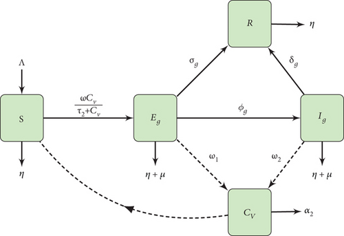
A model with Gumboro pathogen population N_g and the chicken population N_c is developed in this research. Thus, the total population at a given time (t) is N(t) = N_c(t) + N_g(t). Gumboro pathogen population N_g has one compartment consisting of concentration of Gumboro virus in the environment C_V. The chicken population N_c is grouped into four compartments which consist of susceptible chicken S, birds that are at early stages of infection with Gumboro E_g, birds that are in acute stages of infection with Gumboro I_g, and those that will recover from Gumboro disease in both early and acute stages of infections simultaneously R. The model assumes that the bird population recruitment rate to the susceptible compartment will be Λ. The susceptible birds are infected with Gumboro at the rate of ωC_V/τ₂ + C_V. Where ω is the contact rate of susceptible birds with an IBD virus-contaminated environment, τ₂ is the IBD virus concentration in the environment with a 50% probability of Gumboro infections. All bird populations experience natural death at the rate η. Additionally, they die from Gumboro at the rate of μ. The Gumboro-infected birds in both stages of infection shed the virus to the environment at the rates ω₁₋₂ which die at the rate α₂, while σ_g and δ_g are recovery rates for birds at both early and acute stages of infection. Birds at the early stages of Gumboro infections move to the acute stages of infection at the rates ϕ_g.

2.1. Model Assumptions

The model assumptions are as follows:

1.
The bird species that are infected with Gumboro is chicken.
2.
Chickens are recruited into the system by birth or immigration.

2.2. Model Flow Chart and Equations

From Figure 1, the following equations are developed:

(1)

Details are in the caption following the image — **Figure 1**
Open in figure viewer PowerPoint

Flow chart.

3. Basic Properties of the Model

In this section, we discuss the positivity and boundedness of the solutions of the model.

3.1. Positivity of the Solutions of the Model

Theorem 1. There exists a nonnegative solution set {S, E_g, I_g, R, C_V}(t) of model (1) for all t > 0 given that the initial conditions S(0) > 0, E_g(0) ≥ 0, I_g(0) ≥ 0 R(0) ≥ 0, C_V(0) ≥ 0 in have nonnegative values.

Proof 1. From the first equation of system (1), we have

(2)

Equation (2) can be expressed as

(3)

Separating the variables, we obtain

(4)

Integrating on both sides of Equation (4), we have lnS > −(γ_g + η)t + c₁ or

(5)

From Equation (5), it is clear that S(0) = c for t = 0.

Therefore, and as t⟶∞, we have S(t) > 0∀t > 0.

Also from the second equation of system (1)

( )

we have

( )

Solving the above equation by separation of variables, we have

( )

Upon integrating on both sides, we have lnE_g(t) ≥ −(σ_g + ϕ_g + η + μ)t + c:

(6)

Clearly for t = 0, c = E_g(0).

Thus, Equation (6) becomes

( )

and as t⟶∞, we have

Applying the same method to other equations of the system (1), we get

( )

. Thus (S(0) > 0, E_g(0) ≥ 0, I_g(0) ≥ 0, R(0) ≥ 0, C_V(0) ≥ 0) for all t > 0.

3.2. Boundedness of the Solutions of the Model

Let be a feasible region in which the solutions of the total population are bounded, where Ω_C is the feasible region of the solutions of the bird population and that of the Gumboro pathogen population is given by . We show that the solutions of the system (1) are bounded in the feasible region.

The total bird population is N_C given by

( )

Thus, from system (1), we have

(7)

When the birds are not infected, Equation (7) reduces to

(8)

Upon solving Equation (8), we get

(9)

And taking limits as t⟶∞, we have

(10)

Thus, the bird population is bounded in

( )

Considering the last equation of system (1), that is Equation (10), we have

(11)

Upon reduction of Equation (11), we have

(12)

By using the integrating factor, we solve Equation (12) to get

(13)

Taking the limit of Equation (13), as t tends to infinity, gives N_g ≤ Λ(ω₁ + ω₂)/ηα₂. Thus, the Gumboro population is bounded in the region

( )

Since the bird population and Gumboro pathogen population are bounded, then the model will be analyzed in a suitable feasible region

( )

4. Analysis of the Model

4.1. Disease-Free Equilibrium (DFE) Point

The DFE of the system (1) is computed by letting S = S^∗,

, R = R^∗ = 0, and

and setting the right-hand side of the equations of the system (1) equal to zero, then solving the resulting system of equations. Hence, we get

( )

4.2. Reproduction Number for Gumboro Model

The reproduction number R_0g is described as the average number of secondary cases that result from an average initial case in a completely susceptible population in [9]. In our situation, the reproduction number R_0g is the average number of secondary cases resulting from a typical Gumboro infection case in a completely uninfected population. R_0g is found using the Next Generation Matrix approach by [10]. Let the rates of new infections in class j be denoted by f_j, while the rates of chicken transfers into and out of class j are represented by v_j. The Next Generation Matrix is given by FV⁻¹, where F and V are the Jacobian matrices of the vectors f_j and v_j, respectively, at

. The following equations capture the infected population.

(14)

From the system (14), we have

( )

Also, from the system (14), we have

( )

By definition of F and V, we have

( )

and

where

c₂ = σ_g + ϕ_g + η + μc₅ = δ_g + η + μ

Using Mathematica software, the inverse of V is given by

( )

Thus

( )

which implies that the basic reproduction number, R_0g, for the Gumboro model is given by

( )

4.3. Local Stability of DFE

The DFE is locally asymptotically stable if all the real parts of the eigenvalues of the Jacobian matrix of the system (1) at the DFE are all negative.

The Jacobian matrix of the system (1) at the DFE

is given by

(15)

From the Jacobian matrix (15), we have the following characteristic equation:

(16)

In view of Equation (16), λ₁ = −η and λ₂ = −η are the eigenvalues of the Jacobian matrix (15). The other three eigenvalues can be obtained from the following reduced characteristic equation:

(17)

where

( )

It is clear that

( )

and a₂, a₃ > 0 if R_0g < 1

According to Routh–Hurwitz criteria, Equation (17) has roots with negative real parts if a₀ > 0, a₁ > 0, a₂ > 0, a₃ > 0 and a₁a₂ − a₀a₃ > 0. Thus, the DFE of the system of Equation (1) is locally asymptotically stable if the following theorem holds.

Theorem 2. The DFE of the system of Equation (1) is locally asymptotically stable when R_0g < 1 and unstable otherwise.

4.4. Global Stability of DFE

In this section, we use the Castillo–Chavez theorem in [11] to analyse the disease-free state’s global asymptotic stability. To begin, the system (1) must be expressed in the following format:

(18)

where

and

. Uninfected individuals are represented by the components of

, while infected ones are represented by the components of

. The system’s DFE now becomes

. The following two conditions must be met to provide global asymptotic stability.

1.
is globally asymptotically stable (GAS)

(19)

where

is an M-matrix (the off-diagonal components of G are nonnegative) and Ω represents the region where the model makes biological sense. The following theorem holds if the system (18) meets the aforementioned two conditions.

Theorem 3. The DFE is a GAS equilibrium of system (18) provided that R_0g < 1 and the assumptions in Equation (19) are met.

Proof 2. From Theorem 2, the DFE () is locally asymptotically stable when R_0g < 1. Consider

(20)

From Equation (20), we have

(21)

and it follows that

(22)

Thus

( )

Thus, the first and the second conditions in Equation (19) are satisfied since

( )

and

, respectively. Therefore,

has a global asymptotic stability

4.5. Existence of the Endemic Equilibrium Point ()

Theorem 4. There exists a positive endemic equilibrium point for the system of Equation (1) provided that R_0g > 1.

Proof 3. Letting S = S^∗∗, , , R = R^∗∗, and and setting the right-hand side of the equations of the system (1) equal to zero, we get

(23)

Explicitly solving for values of , we obtain

(24)

Thus, a positive exists if R_0g > 1.

4.6. Local Stability of Endemic Equilibrium

We use the center manifold theory as described in [12] to assess the stability of the endemic equilibrium, , because evaluating the eigenvalues of the Jacobian matrix of system (1) at the endemic equilibrium is complicated. Theorem 4.1 in [12] outlines the procedure of analyzing the local stability of endemic equilibrium in a nutshell. The coefficients, a and b of the normal form, are two key quantities in expressing the system’s dynamics on the center manifold theory as described in Theorem 4.1 in [12]. According to part (iv) of Theorem 4.1 in [12], if a < 0 and b > 0, the endemic equilibrium is locally asymptotically stable for R_0g > 1 but close to 1.

Theorem 5. The endemic equilibrium is locally asymptotically stable if R_0g > 1

Proof 4. By using the center manifold theory, Theorem 4.1 in [12], we rename the variables in the system (1) as S = x₁, E_g = x₂, I_g = x₃, R = x₄, and C_V = x₅ such that . Further, by using , the system (1) can be written in the form dX/dt = F(X), with , as follows:

(25)

Suppose that ω = ω^∗ is a bifurcation parameter when R_0g = 1, solving for ω^∗ for R_0g = 1 from

( )

we have

(26)

The Jacobian matrix of the system (25) at with ω = ω^∗ is given as

(27)

The Jacobian matrix (27) has zero eigenvalues close to ω = ω^∗; thus, the center manifold theory is utilized to examine the dynamics of the system. Let , a right eigenvector associated with the Jacobian matrix (Equation (27)), be close to ω = ω^∗, then

(28)

Solving system (28), we get

(29)

Also, let , a left eigenvector associated with the Jacobian matrix (Equation (27)), be close to ω = ω^∗, such that

(30)

Solving system (30), we obtain

(31)

Using the formula described in [12], we compute a and b:

( )

To get the bifurcation coefficient a, we first obtain the nonzero partial derivatives of the model system (25) evaluated at . Thus, it is evident that

(32)

so that

(33)

Using Equations (29) and (31), Equation (33) can be written as

( )

For the coefficient b, we have the following nonzero partial derivatives of the model system (25) evaluated at :

(34)

Hence,

(35)

Using Equations (29) and (31), Equation (35) can be written as

( )

Since a < 0 and b > 0, it follows that the endemic equilibrium is locally asymptotically stable if R_0g > 1.

4.7. Global Stability of the Endemic Equilibrium Point

Theorem 6. The endemic equilibrium point of the system (1) is GAS if R_0g > 1.

Proof 5. We have shown in Section (4.5) that the endemic equilibrium point exists when R_0g > 1. Using the Poincaré–Bendixson theorem, the global stability of the endemic equilibrium point is investigated [13]. It follows from Dulac’s multiplier, 1/SE_gI_gRC_V, that

(36)

Due to the fact that Ω is positively invariant and the endemic equilibrium exists whenever R_0g > 1, there are no periodic orbits in Ω according to Dulac’s criterion. From the Poincaré–Bendixson theorem, it follows that all solutions of the limiting system originating in Ω remain in Ω for all time t. The absence of periodic orbits suggests that whenever R_0g > 1, the special endemic equilibrium of the Gumboro model is GAS.

5. Numerical Simulation

Numerical simulations to prove the theoretical results for the Gumboro disease mathematical model were carried out using MATLAB ode 45 solver. This was made possible by the use of some parameters in the literature and others that were estimated or assumed as shown in Table 1.

Table 1. Parameter description.

Parameter	Value	Source
Λ	10	[7]
ω	0.000143 (0.000143–0.0143)/day	[7]
τ₂	0.009/day	Assumed
η	0.0001543/day	[7]
μ	0.032143/day	[7]
ω₁	0.008 (0.008–0.08)/day	Assumed
ω₂	0.009 (0.009–0.09)/day	Assumed
α₂	0.0900982/day	Assumed
θ_g	0.0039 (0.0039–0.39)/day	Assumed
σ_g	0.0165/day	[8]
δ_g	0.021429/day	[7]
ϕ_g	0.033/day	[8]

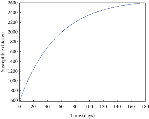
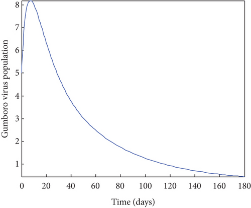
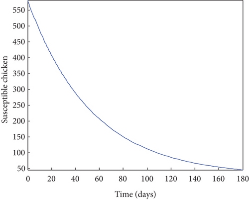
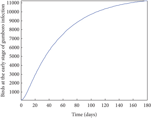
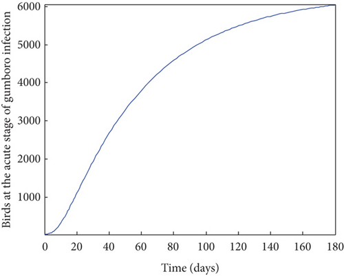
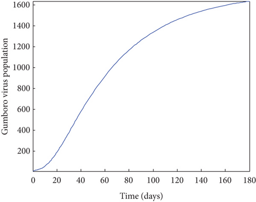
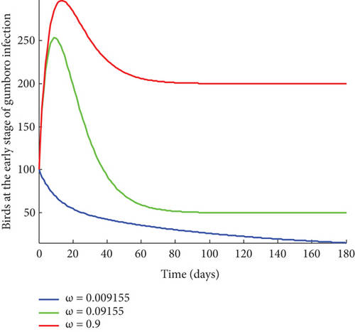
From Figure 2, it was shown that the number of birds at early stages of infection, acute stages of infection, and the pathogen population converges to zero while the susceptible birds’ population tends to a constant λ/η when R_0g < 1 which implies that whenever Gumboro disease dies out, only the susceptible chicken would remain. Figure 3 also shows that birds at early and acute stages of infection together with the pathogen population tend towards the endemic equilibrium point when R_0g > 1 while the susceptible birds converge to zero indicating that Gumboro disease remains endemic. From Figure 4, it was shown that birds at early stages of infection increase with the increase in the contact rate of susceptible to Gumboro disease-contaminated environment.

6. Conclusion

A mathematical model of Gumboro disease transmission dynamics was formulated in this paper. The disease-free and endemic equilibrium points were determined, and the reproduction number was derived. The findings showed that Gumboro disease dies out whenever R_0g < 1 and persists in the chicken population whenever R_0g > 1. Also, it was realized that minimizing the contact rate of chicken to a contaminated environment lowers cases of infections in a population. These numerical simulation findings were found to be in harmony with the theoretical stability analysis results.

Conflicts of Interest

The authors declare no conflicts of interest.

Author Contributions

All the authors collaborated in carrying out this study. Author I.C. designed the study, author J.S.M. wrote the first draft of the manuscript and performed the mathematical analysis of the study and the literature review, and author W.N.M. performed the numerical simulation. All authors read and approved the final manuscript.

Funding

The authors received no specific funding for this work.

Acknowledgments

The authors appreciate the ample time given by their respective universities in writing this manuscript.

Open Research

Data Availability Statement

All data is provided in this paper.

References

1 Daraj J., Infectious bursal disease in poultry, 2019, https://www.msdvetmanual.com/poultry/infectious-bursal-disease/infectious-bursal-disease-in-poultry, on 23/6/2021.
Google Scholar
2 George T. and Jessica B. W., Infectious Bursal Disease (GUMBORO) in Backyard Chicken, 2018, Mississippi state university publication number P3211.
Google Scholar
3 Mengesha M. and Tsega W., Phenotypic and genotypic characteristics of indigenous chickens in Ethiopia: a review, African Journal of Agricultural Research. (2011) 6, no. 24, 5398–5404.
Google Scholar
4 Mutinda W. U., Nyaga P. N., Njagi L. W., Bebora L. C., and Mbuthia P. G., Gumboro disease outbreaks cause high mortality rates in indigenous chickens in kenya, Bulletin Health and Production Africa. (2018) 61, 571–578.
Google Scholar
5 Mishra B. K. and Sinha D. N., A mathematical model on avian influenza with quarantine and vaccination, Journal of Immunological Techniques & Infectious Diseases. (2016) 5, no. 4.
Google Scholar
6 Uwakwe J. I., Inyama S. C., and Omame A., Mathematical model and optimal control of New-Castle disease (ND), Applied and Computational Mathematics. (2020) 9, no. 3, 70–84, https://doi.org/10.11648/j.acm.20200903.14.
10.11648/j.acm.20200903.14
Google Scholar
7 Omollo E. A. and Kimathi G., Formulation of a mathematical model for the transmission dynamics of infectious bursal disease (IBD), incorporating effects of environmental factors, Asian Research Journal of Mathematics. (2020) 16, no. 9, 20–35, https://doi.org/10.9734/arjom/2020/v16i930217.
10.9734/arjom/2020/v16i930217
Google Scholar
8 Uwakwe J. I., Inyama S. C., Emerenini B. O., and Nse C. A., Mathematical and Control Model of Bursal Disease (Ibd), 2019, IOSR Journal of Mathematics (IOSR-JM) e-ISSN.
Google Scholar
9 Diekmann O. and Heesterbeek J. A. P., Mathematical Epidemiology of Infectious Diseases: Model Building, Analysis and Interpretation. Vol. 5, 2000, John Wiley & Sons.
Google Scholar
10 Van den Driessche P. and Watmough J., Reproduction numbers and sub-threshold endemic equilibria for compartmental models of disease transmission, Mathematical Biosciences. (2002) 180, no. 1-2, 29–48, https://doi.org/10.1016/s0025-5564(02)00108-6, 2-s2.0-0036845274, 12387915.
10.1016/S0025-5564(02)00108-6
CAS PubMed Web of Science® Google Scholar
11 Castillo-Chavez C., Feng Z., and Huang W., On the computation of R₀ and its role on global stability, Mathematical Approaches for Emerging and Reemerging Infectious Diseases. (2002) 125, 229–250, https://doi.org/10.1007/978-1-4757-3667-0-13.
10.1007/978-1-4757-3667-0_13
Google Scholar
12 Castillo-Chavez C. and Song B., Dynamical models of tuberculosis and their applications, Mathematical Biosciences and Engineering. (2004) 1, no. 2, 361–404, https://doi.org/10.3934/mbe.2004.1.361.
10.3934/mbe.2004.1.361
PubMed Web of Science® Google Scholar
13 Adebimpe O., Moses B. O., and Okoro O. J., Global stability analysis of a SEIR epidemic model with saturation incidence rate, International Journal of Mathematical Sciences. (2014) 34, no. 1.
Google Scholar

All articles

Mathematical Modeling of the Transmission Dynamics of Gumboro Disease

Abstract

1. Introduction

2. Model Formulation

2.1. Model Assumptions

2.2. Model Flow Chart and Equations

3. Basic Properties of the Model

3.1. Positivity of the Solutions of the Model

3.2. Boundedness of the Solutions of the Model

4. Analysis of the Model

4.1. Disease-Free Equilibrium (DFE) Point

4.2. Reproduction Number for Gumboro Model

4.3. Local Stability of DFE

4.4. Global Stability of DFE

4.5. Existence of the Endemic Equilibrium Point ()

4.6. Local Stability of Endemic Equilibrium

4.7. Global Stability of the Endemic Equilibrium Point

5. Numerical Simulation

6. Conclusion

Conflicts of Interest

Author Contributions

Funding

Acknowledgments

Open Research

Data Availability Statement

References

Figures

References

Information

About Wiley Online Library

Help & Support

Opportunities

Connect with Wiley

Mathematical Modeling of the Transmission Dynamics of Gumboro Disease

Abstract

1. Introduction

2. Model Formulation

2.1. Model Assumptions

2.2. Model Flow Chart and Equations

3. Basic Properties of the Model

3.1. Positivity of the Solutions of the Model

3.2. Boundedness of the Solutions of the Model

4. Analysis of the Model

4.1. Disease-Free Equilibrium (DFE) Point

4.2. Reproduction Number for Gumboro Model

4.3. Local Stability of DFE

4.4. Global Stability of DFE

4.5. Existence of the Endemic Equilibrium Point ()

4.6. Local Stability of Endemic Equilibrium

4.7. Global Stability of the Endemic Equilibrium Point

5. Numerical Simulation

6. Conclusion

Conflicts of Interest

Author Contributions

Funding

Acknowledgments

Open Research

Data Availability Statement

References

Figures

References

Related

Information