Enhancing Load Forecasting Accuracy in Smart Grids: A Novel Parallel Multichannel Network Approach Using 1D CNN and Bi-LSTM Models
Abstract
Load forecasting plays a pivotal role in the efficient energy management of smart grid. However, the complex, intermittent, and nonlinear smart grids and the complexity of large dataset handling pose difficulty in accurately forecasting loads. The important issue is considering the cyclic features, which have not yet been adequately addressed through the trigonometric transformations. Furthermore, using long short-term memory (LSTM) or 1D convolution neural network (1D CNN) and existing hybrid models involve stacked CNN-LSTM architectures, employing 1D convolutions as a preprocessing step to downsample sequences and extract high- and low-level spatial features. However, these models often overlook temporal features, emphasizing higher-level features processed by the subsequent recurrent neural network layer. Therefore, this study considers a novel approach to independently process features for spatial and temporal characteristics using a parallel multichannel network comprising 1D CNN and bidirectional-LSTM (Bi-LSTM) models. The proposed model evaluated the National Transmission and Dispatch Company (NTDC) load dataset, with additional assessment on two datasets, American Electric Power and Commonwealth Edison, to ensure its generalizability. Performance evaluation on the NTDC dataset yields results of 3.4% mean absolute percentage error (MAPE), 513.95 mean absolute error (MAE), and 623.78 root mean square error (RMSE) for day-ahead forecasting, and 0.56% MAPE, 94.84 MAE, and 115.67 RMSE for hour-ahead load forecast. The experimental results demonstrate that the proposed model outperforms stacked CNN-LSTM models, particularly in forecasting hour- and day-ahead loads. Moreover, a comparative analysis with previous studies reveals superior performance in reducing the error gap between predicted and actual values.
1. Introduction
The smart grid has grown to accommodate large-scale renewable energy and incorporate the communication network into managing the protracted frequency and voltage of the smart grid at various levels [1, 2]. In the smart grid, most of the reliance is on the short-term load forecasting (STLF) to assess the security of the power systems, predict the load to schedule the generation, and provide dispatcher information in the short term. STLF forecasts the electrical load, which ranges from hours to days. The load prediction for the STLF function involves several functions that include economic trends, cyclical trends, weather patterns, and unforeseen factors [3]. Economic realities play out in boosting a facility by constructing new buildings and laboratories. There are weekly and daily cycles, and regarding load estimates, seasonal fluctuations significantly affect the results and vacations. HVAC is considered a climate-dependent load in different electrical systems, even in facilities with considerable electrical loads smaller than the systems controlling them, usually in industrial or Institutional electrical systems. In addition, the load level of a facility can be altered significantly by events such as lengthy human absence, planned and unplanned power systems, and other outages [4]. Further, the AI-based forecasting mechanisms enhance the load forecasting models compared to general procedures to minimize discrepancies and augment systems’ reliability. Likewise, in the smart grid environment, such an STLF solution is needed for the customer due to its dependency on outside factors that are highly intertwined and nonlinear. In this regard, many studies have been undertaken on the fundamentals and application of deep learning algorithms to build accurate and robust load forecasters.
1.1. Literature Review
The study has extensively reviewed the literature on smart power systems’ STLF models. For instance, Morais et al. [5] presented a unique hybrid system based on the weighted support vector regression technique (LWSVR) and the grasshopper optimization algorithm (MGOA). Parameters for the LWSVR were derived using the MGOA method applied to various real-world datasets. Rodríguez et al. [6] trained the recurrent neural network (RNN) topology utilizing an algorithm based on the Levenberg–Marquardt technique to devise a forecaster for the smart grid, ensuring a more stable operational behavior. Sensitivity analysis was conducted, and accuracy was determined using simple error matrices, showing a 0.5% error in 97% of the day’s output. Aly [7] presented the STLF method utilizing a blend of diverse models and integrating clustering methods to elevate overall system effectiveness and quality. These models comprise varying combinations of Kalman filtering, wavelet, and artificial neural network (WNN and ANN) techniques. Simulation results showcase the superior performance of the proposed models. The effectiveness of the proposed approach is validated by utilizing datasets from two distinct locations: Egypt and Canada. The correlation between electrical load and weather parameters is studied in [8, 9], and machine learning (MLR) technique is used to predict the short-term load of the power grid. While considering the acceptable limits of error, the load level was successfully forecasted for a week using the accuracy metric of mean absolute percentage error (MAPE). The reported MAPE for the 168-hr forward load forecasting data is 3.99%. Debnath and Mourshed [10] introduced a nonparametric regression method for STLF, relying on a probability density function and various influencing variables, such as time and weather. With minimal parameters, the approach depends on past data accuracy. The study assessed temperature forecast impacts, highlighting potential errors. In [11], an STLF technique integrates the lifting scheme with autoregressive integrated moving average (ARIMA) models. The lifting technique divides the load series into subseries and projects them using ARIMA models, utilizing the Coiflet 12 wavelet. The method, evaluated with Tai Power load types, surpasses traditional ARIMA and BPN techniques in feasibility and efficiency. Performance metrics like MAPE, mean absolute error (MAE), and root mean square error (RMSE) validate the effectiveness of the proposed technique and determine its efficacy in load forecasting. In [12], a practical and accurate commutable forecasting system was developed, providing user-friendly hourly predictions for MW hr demand with lead times ranging from 1 to 24 hr. The approach, grounded in real-world considerations, incorporated 2 years of hourly load data, tests, and adjustments for holidays and weather disruptions. Operating on overall system demand, the system generated 24 predictions every hour. Initial coefficients were estimated from the first 1,680 hr, and forecasts were computed every fifth hour to optimize computational efficiency. The system exhibited a typical 2%–4% of average load standard error for lead times from 1 to 24hr, with forecast mistakes following a normal distribution. Yang et al. [13] proposed a Novel Technique of SVR, which is based on the sequential grid approach, to enhance the accuracy of the STLF process. The study conducted a simulation analysis in which the grid parameters were optimized using the proposed grid algorithm, significantly improving performance by outperforming conventional SVR models. In [14, 15], a novel STLF method was presented using clustering and ANN that enhanced real-time forecasting accuracy by grouping historical load and temperature data and employing the backpropagation method. The clustered approach showed reduced maximum and average percentage errors across all days of the week compared to a nonclustered system, emphasizing the effectiveness of clustering in improving load prediction precision with ANN. Kong et al. [16] focused on the progression of shallow and deep neural networks, encompassing multilayer perceptron, long-short term memory, and gated recurrent unit, to tackle STLF.
In [17], a practical and accurate commutable forecasting system is developed, providing user-friendly hourly predictions for MWh demand with lead times ranging from 1 to 24 hr. The approach, grounded in real-world considerations, incorporates 2 years of hourly load data, tests, and adjustments for holidays and weather disruptions. Operating on overall system demand, the system generates 24 predictions every hour. Initial coefficients are estimated from the first 1,680 hr, and forecasts are computed every fifth hour to optimize computational efficiency. The paper [18] introduces an SVR base model for load forecasting, trained on load and weather data, without the need for submetering data. The model’s simplicity facilitates quick and straightforward computation on a computer, offering advantages to demand response participants. In [19], the study focuses on the progression of shallow and deep neural networks, encompassing multilayer perceptron, long-short term memory, and gated recurrent unit, to tackle STLF. The research work in [20] introduces a deep learning framework centered on long short-term memory (LSTM) for predicting short-term electric loads for individual units. It emphasizes the advantages of merging CNN and LSTM layers within a hybrid structure. Employing data acquired from the Australian Government’s Smart Grid Smart City project, the investigation exhibits heightened precision in forecasting energy usage for individual households. The combined CNN-LSTM model outperforms the standalone LSTM model, showcasing its ability to precisely predict energy consumption, particularly in scenarios marked by anomalies and varied load patterns. In [21], the paper presents an LSTM neural network forecasting model for short-term electrical demand, offering both single-step and intraday rolling horizon predictions. The model incorporates weather data and significantly enhances accuracy by including a definite feature vector with time-of-day, holiday flag, and day-of-week indices.
1.2. Research Gap and Paper Contribution
The aforementioned literature covered a broad range of STLF models aimed at addressing issues related to load forecasting. However, a persistent gap still exists. For instance, the issue of cyclic features has not been covered in detail, particularly regarding trigonometric transformations. Additionally, utilizing LSTM and 1D convolutional neural networks (1D CNN) alongside existing hybrid models entails the employment of stacked CNN-LSTM architectures. These architectures incorporate 1D convolutions as a preprocessing stage to downsample sequences and extract both high- and low-level spatial features. However, it is noteworthy that these models frequently neglect temporal features, instead prioritizing higher-level features processed by subsequent RNN layers.
Keeping in view the aforementioned issues, this study proposes a deep learning technology that integrates different layers, including LSTM, CNN, and Bi-LSTM. Various preprocessing methods are devised to enhance the model’s performance. The employed Bi-LSTM layer considers past and future contexts within the sequential data stream and captures bidirectional temporal features. Further, the parallel operation performs two different tasks. Segment 1 extracts the spatial features using the CNN method, while the second segment captures the temporal characteristics using the Bi-LSTM and LSTM methods. Thus, the aggregated operation further enhances the model’s performance by handling spatial and temporal features individually, subsequently improving the efficiency of the LSTM forecaster.
1.3. Structure of the Paper
The paper is structured in the following manner: Section 2 illustrates the proposed model, while Section 3 presents the different data preprocessing steps, including the train test split, data cleaning, feature extraction, and development of the input matrix. Section 4 presents the results and discussion, explaining the model’s training and the hour-ahead and day-ahead scenarios. Section 5 concludes the key findings of the study.
2. Proposed Methodology
The proposed model is shown in Figure 1, with a CNN layer followed by a Max-Pooling layer to get important features and dropout to reduce overfitting. The first bidirectional layer collects long-lasting temporal correlations in power usage in the forward and backward directions. The next two LSTM layers are quite good at extracting long-term positive interdependencies. Combined with a 1D CNN, the LSTM network runs concurrently. In Figure 1, the LSTM, “30” indicates the number of units; in CNN, “32” shows the number of filters, and “6” indicates the kernel size.
The temporal load data global characteristics are captured in the convolutional route using a large kernel in the 1D CNN. This calculated decision makes it easier for the model to identify broad trends and patterns that run the whole length of the input sequence. However, the next 1D CNN layer’s smaller kernel concentrates on localized characteristics, allowing the model to identify minute details and minuscule variances in the input. The intended discrepancy in kernel widths enables the model to better understand the underlying dynamics of load forecasting by thoroughly evaluating both coarse- and fine-grained input features. Collecting temporal correlations within the load series across time falls to the LSTM and Bi-LSTM layers that make up the second parallel pathway shown in Figure 1. In this configuration, Bi-LSTM extracts the enhanced temporal features from temporal data as the Bi_LSTM can store the temporal data features in either direction. However, the LSTM is famous for sequential data, so its hybridization enhanced the results. Bi-LSTM is a technique for gathering short-term and long-term information in backward and forward passes to understand sequences’ relationships keenly. This technique thoroughly explains the contextual linkages within the temporal sequence.
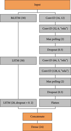
The subsequent LSTM layers, with their various units and dropout mechanisms, are designed to discover and know the time-related properties and long-term dependencies required for the exaction of the short-term load prediction. The planned integration of convolutional and recurrent layers in the two parallel paths allows for a joint evaluation of spatial and temporal features, thereby equipping the model to identify and anticipate load patterns properly. The complex architecture of the model essentially combines large and small kernels in the 1D CNN route with LSTM and Bi-LSTM layers in a parallel pathway to mix different filters and network configurations. The detailed process for developing the input Matrix is explained in Section 3.
Bi-LSTM enhances the simple LSTM by passing the input sequence in both forward and backward directions, with forward and backward LSTM layers together outputting the result. Although unidirectional LSTM can fully use historical information, it can not use future information in its prediction work [22]. However, the Bi-LSTM method will consider past and future data, making the model’s forecasted values more accurate. Bi-LSTM could be more effective than simple LSTMs and capable of enhanced performance in activities involved in load forecasting because it considers both the order of the input data and the order of the events. Nevertheless, in the case of CNNs, it may only be insufficient to capture the temporal dependencies pertinent to time series that are chargeable for prognostic tasks requiring future values for prediction. Therefore, the proposed solution incorporates RNN and combines CNN with LSTM to enhance performance and accuracy during data processing [23].
3. Data Preprocessing
For best learning, the data must be effectively preprocessed before being used for model training. A well-prepared dataset improves a model’s capacity to identify trends and connections. The main preprocessing procedures are training test split, data cleaning, high-level feature extraction, and preparing the data into a 3D format (samples, time steps, and features) suitable for model training. Figure 2 shows the complete preprocessing flowchart. These steps have thoroughly been explained in the following subsections.
3.1. Train Test Split
The train-test split is the first step in data preparation; it entails splitting the dataset into separate groups for testing, validation, and training. This data splitting is essential for appropriately evaluating the model’s generalization performance. Seventy percent of the data is usually set aside for training, which enables the model to discover patterns and correlations within the dataset.

Twenty percent of the data comprise the next subset set aside for validation. During the training phase, this validation set is essential for adjusting the model’s hyperparameters and avoiding overfitting. Finally, the testing subset will use the final 10% of the data. Crucially, this phase is carried out right from the beginning to reduce the possibility of data leaking, guaranteeing that data from the testing set does not unintentionally affect the model while it is being trained. This preventive step is essential to assess the model’s performance on untested data, improving the MLR model’s resilience and dependability.
3.2. Data Cleaning
Repairing or deleting erroneous, incomplete, or duplicate data from a dataset is called data cleaning or cleansing. Data cleansing must come first in your workflow. When working with huge datasets and combining multiple data sources, one will likely duplicate or incorrectly classify data. Inaccurate or wrong data will degrade the quality of your algorithms and results, rendering them unreliable. Figure 3 demonstrates the steps involved in data cleaning [24]. All essential procedures are made for National Transmission and Dispatch Company, Pakistan (NTDC), American Electric Power (AEP), and Commonwealth Edison (COMED) hourly load consumption statistics while maintaining or improving data quality.

Some preliminary information of all these datasets is summarized in Table 1 [25].
| Parameter | Values | ||
|---|---|---|---|
| NTDC | AEP | COMED | |
| Samples with NaN | 2 | 0 | 0 |
| Minimum load before preprocessing | 500 | 121,273 | 66,497 |
| Maximum load before preprocessing | 24,786 | 121,296 | 66,504 |
| Missing values in the data | 120 | 27 | 11 |
| Redundant | 53 | 4 | 4 |
| Outliers | 10 | — | — |
| Samples after preprocessing | 46,728 | — | — |
| Minimum load after preprocessing | 1648 | — | — |
| Maximum load after preprocessing | 22,696 | — | — |
3.2.1. Missing Values Handling
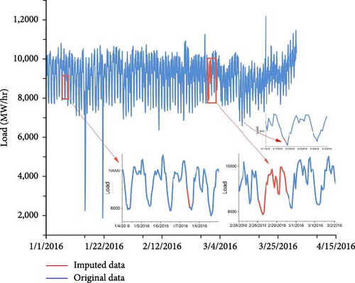
All three datasets, namely NTDC, AEP, and COMED, contain instances of missing data. These missing values are classified into three types: single missing values, two consecutive missing values, and many consecutive missing values. Specific techniques were applied to address each category to maintain the inherent trends in the data. For single missing values, linear interpolation was employed, utilizing the time parameter to ensure accurate estimation. In the case of two consecutive missing values, the missing values were filled by incorporating the mean of the surrounding data points. Similarly, the approach involved averaging the load data from 2 weeks before and 2 weeks ahead for datasets with many consecutive missing values. This methodology is illustrated in Figure 4, depicting the approach applied to datasets with a higher occurrence of consecutive missing values.
3.2.2. Outlier Handling
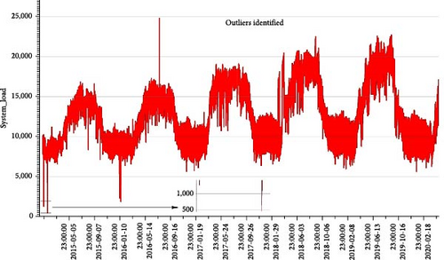
The NTDC dataset exhibits the presence of 10 outliers, as detailed in Table 1 and visually represented in Figure 5. In contrast, the remaining two datasets, AEP and COMED, primarily showcase higher outliers occurring at regular intervals. This pattern suggests that these higher values in the latter datasets should not be treated as outliers, as they align with inherent consumption patterns. However, in the case of the NTDC dataset, the identified outliers are noteworthy and potentially attributed to unique events, such as the blackout in Pakistan in 2015, as illustrated in Figure 6(a).
A systematic process is used to find and remove outliers to strengthen the dataset’s resilience and dependability, as shown in Figures 6(a) and 6(b). This procedure applies the preprocessing methods previously covered to outliers and handles them similarly to missing values. The main objective is to put into practice a thorough strategy that ensures the data’s future analysis and modeling appropriately represent the underlying consumption patterns. This technique lessens the effect of abnormal data points by handling outliers the same way as missing values. The dataset is thoroughly refined by incorporating them into the preprocessing approaches that were previously explained. This significantly enhances the representation’s correctness and resilience, making the dataset more suitable for analytical purposes. This method ensures the dataset’s trustworthiness and promotes a detailed understanding of consumption patterns—essential for insightful and trustworthy investigations.


3.2.3. Redundant Handling
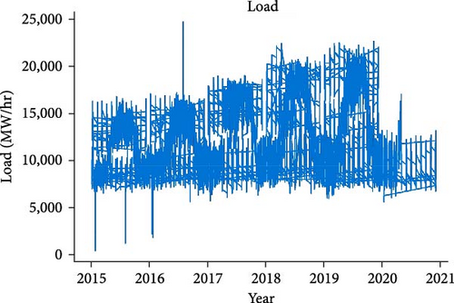
Redundant data, characterized by duplicates or repetitions, are identified within NTDC, AEP, and COMED datasets. The graphical representation in Figure 7 sheds light on the impact of redundant data, specifically within the NTDC dataset. A meticulous two-step process is implemented across all datasets to tackle this issue effectively. In the initial step, the redundant data undergo a resampling procedure. In the second step, the last instance of the duplicated data is systematically removed. This ensures that all datasets are thoroughly cleansed, eliminating any trace of duplicate entries. This approach not only addresses the challenge posed by redundant data but also enhances the overall integrity and accuracy of the datasets.
3.3. Feature Extraction
Feature extraction is critical for extracting relevant patterns and information from unprocessed data and improving knowledge of the underlying relationships. Important features from the dataset were extracted for our study, as shown in Figure 8. Figure 8 graphically illustrates some retrieved attributes and information on their distributions and variances. A correlation analysis was conducted to investigate the interdependencies among these factors further, and Table 2 demonstrates how these attributes connect with system load. The correlation coefficients between different pairs of characteristics are summarized in Table 2, providing a thorough understanding of how they relate to the system load. Figure 8(b) clarifies the significant association with the summer season. In particular, the load’s overall mean always gets closer to its maximum value throughout June, July, and August. This well-thought-out study emphasizes the obvious relationship between certain characteristics and the system load, and Figure 8(b) graphically highlights the summer’s significant impact on load dynamics.
| Feature | Spearman correlation |
|---|---|
| NTDC | |
| Month of year | 0.226 |
| Day of week | −0.018 |
| Hour of day | 0.148 |
| Holiday | −0.012 |
| Winter peak | −0.134 |
| Summer peak | 0.254 |
| Spring peak | 0.023 |
| Autumn peak | 0.052 |
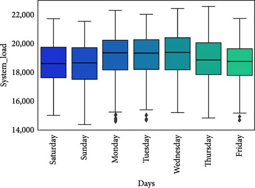
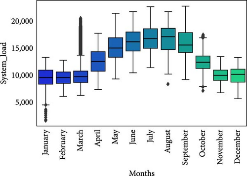
A higher correlation coefficient suggests a stronger linear association between the two features. Correlation analysis helps identify which features may affect each other and can guide further steps in model development. This integrated feature extraction, visualization, and correlation analysis approach contributes to a more shaded understanding of the dataset and forms the basis for constructing effective forecasting models. Further, features are transformed according to their nature, as shown in Figure 2, before making the input matrix.
3.4. Input Matrix
- (a)
Define Parameters: This shows the establishment of key parameters, specifically determining the size of the input window (indicating the number of time steps considered as input) and specifying the size of the output window (representing the number of time steps projected into the future).
- (b)
Create Input–Output Pairs: A systematic progression involves sliding the input window through the time series data. The input window is extracted at each position as features, and the subsequent time step/steps are identified as the output. This process is iteratively executed until the last sample of the time series data.
- (c)
Organize Data into 3D Array: The resulting input–output pairs are organized into a 3D array structure. This array is configured with dimensions corresponding to the number of samples, the size of the input window, and the number of features. The resulting 3D representation facilitates the incorporation of temporal dependencies, enabling a comprehensive analysis of the time series data within an MLR framework.
4. Result and Discussion
To train the model, the experiments were conducted on a system with the following hardware specifications: an Intel 64 Family 6 Model 158 Stepping 10 Genuine Intel CPU with multiple cores operating at a frequency of 2,601.0 MHz, 31.85 GB of RAM, and Windows 10. We employed an NVIDIA GeForce RTX 2080 with Max-Q Design to ensure optimal GPU performance, boasting 8,192.0 MB of memory, with the GPU driver version 54633. On average, each experiment took around 16 min to complete. These robust hardware setups provided a solid foundation for our computational activities, ensuring efficient and reliable performance throughout the experiments.
4.1. Model Training
- (i)
The model undergoes training for 60 epochs in the initial phase, utilizing a batch size of 512. During this training period, a learning rate of 10−3 is applied. A crucial aspect of this training process involves incorporating a Keras callback mechanism designed to save the best-performing model. The validation loss serves as the criterion for selecting the optimal model, guaranteeing that the model chosen shows a decrease in validation loss compared to the previous stage.
- (ii)
In the subsequent phase, the optimal model that was previously saved is reloaded, and a refinement is implemented by reducing the learning rate to 10−4. When this changed model is retrained, the optimal model remains intact.
- (iii)
At this stage of the process, the model is further optimized by reducing its rate of learning to 10−5. Afterward, the models are considered the best to perform in this setup. Thus, the model’s overall performance is improved using different training stages and learning rates and storing the optimized model at each step.
KERAS with backend TENSOLFLOW, a reliable neural network framework, is utilized to build these models. In addition to ensuring dependability, this choice of framework and backend shows a dedication to utilizing cutting-edge technologies in the industry. Moreover, the best-saved model is used to analyze the test data, and validation loss is monitored continuously. The load estimates for the hourly and day-ahead periods depend upon a 24-hr load period.
4.2. Hour-Ahead Forecasting
Hourly load forecasting is a crucial part of energy management systems that guarantees the stability and effectiveness of power networks. Precise forecasts facilitate the distribution of resources and load balancing by utilities, changing the overall system performance. Recently, there has been a growing interest in developing advanced forecasting models to increase the accuracy of hour-ahead load estimates. Figure 9 displays the output of our recommended forecasting model and two state-of-the-art models detailed in [26, 27]. The models are evaluated on three distinct datasets: AEP, COMED, and NTDC. The performance of these models was assessed using three crucial assessment metrics: MAPE, RMSE, and MAE. Our proposed model demonstrated good prediction accuracy on the AEP, COMED, and NTDC datasets, with MAPE values of 0.66, 0.5, and 0.56, respectively. This outstanding result outperforms CNN-LSTM-a and CNN-LSTM-b in all three datasets, demonstrating the efficacy of our methodology. The results clearly show that our proposed model performs better than the stacked CNN-LSTM models given in [26, 27], providing compelling evidence of its higher forecasting abilities.
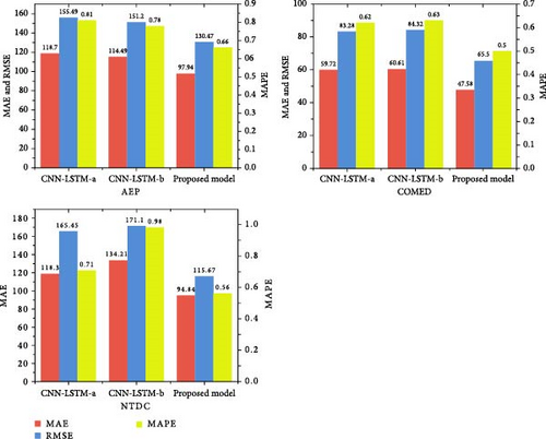
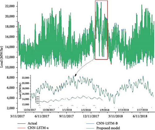
Figure 10 provides additional visualization of our model’s forecasting skills by comparing the anticipated values to real load values and those of other comparator models. The validity and reliability of our suggested strategy are strengthened by this extra representation, which improves our comprehension of the model’s efficiency in collecting and forecasting hour-ahead load patterns.
4.3. Day-Ahead Forecasting
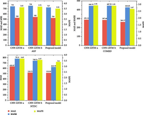
Forecasting models must be successful for energy utilities to plan and distribute resources as efficiently as possible in day-ahead load forecasting. Figure 11 compares our proposed day-ahead forecasting model to two cutting-edge algorithms published in [27], employing three separate datasets, and the results are outstanding. While our recommended model and the comparative model from [27] exhibit practically identical MAPE values on the AEP dataset, it is crucial to remark that there is a clear difference between RMSE and MAE. The difference between RMSE and MAE demonstrates how effectively our model predicts the future by minimizing forecasting mistakes and inconsistencies in the AEP dataset. It is important to mention that the RMSE and MAE analysis is significant since it provides information related to the accuracy of the proposed forecaster, which reduces the error with the actual data compared to the comparator model, as mentioned in [27]. In day-ahead forecasting, which has utilized the date set of AEP, COMED, and NTDC, the generated MAPE values were 3.5, 2.67, and 3.4, respectively, showing the precision of the proposed model in delivering exact day-ahead load estimations across multiple datasets. Further, the MAPE value, which has the least value among the others, when compared to the comparison model from [27], shows the model’s forecasting accuracy with a high degree of accuracy. This excellent result validates our day-ahead forecasting model’s high technical performance and gives energy utilities a useful tool for efficient day-ahead load planning and decision-making.
5. Conclusions
This study proposed an STLF technique for a smart grid using a CNN, Bi-LSTM, and LSTM. To enhance the performance, all the available features are treated separately by CNN and Bi-LSTM, followed by LSTM. The proposed model, having parallel paths for feature extraction, outperforms the stacked CNN-LSTM networks. Compared with other models, the proposed model is tuned for multistep forecasting, which gives good results for both single and multistep forecasting on real-time AEP, NTDC, and COMED datasets. The results presented for hour-ahead and day-ahead forecasting indicate that our proposed method efficiently extracts rich feature representations due to its parallel path structure. This is evident from simulations, where the proposed model achieves the lowest values of MAE, RMSE, and MAPE at 3.4%, 513.95%, and 623.78% for day-ahead forecasting, and 0.56%, 94.84%, and 115.67% for hr-ahead load forecasting, compared to stacked CNN-LSTM models.
In future work, the effectiveness of the proposed approach could be further improved by incorporating temperature data, which may contribute additional contextual information. Consideration might be given to substituting the current CNN architecture with a state-of-the-art alternative, moving away from stacked CNN layers for potential performance enhancements. Intelligent preprocessing techniques could be explored to refine the model’s understanding of temporal dependencies, such as incorporating data from the same hour from the last day, week, or month into the historical context. Moreover, adapting the model to enable probabilistic forecasting offers a promising avenue for enhancing predictive capabilities and capturing uncertainty in the forecasting process.
Conflicts of Interest
The authors declare that they have no conflicts of interest.
Authors’ Contributions
Conceptualization was handled by Syed Muhammad Hasanat, Rehmana Younis, Muhammad Talha Ejaz, Kaleem Ullah, and Zahid Ullah. Data curation was performed by Syed Muhammad Hasanat, Muhammad Haris, and Hamza Yousaf. Formal analysis was carried out by Sadia Watara, Kaleem Ullah, and Zahid Ullah. Investigation responsibilities were assumed by Muhammad Talha Ejaz, Muhammad Haris, Hamza Yousaf, Kaleem Ullah, and Zahid Ullah. The methodology was devised by Syed Muhammad Hasanat, Rehmana Younis, and Kaleem Ullah. Project administration was handled by Saad Alahmari, Muhammad Haris, and Zahid Ullah. Resources were provided by Hamza Yousaf, Sadia Watara, and Saad Alahmari. Software resources were managed by Syed Muhammad Hasanat, Saad Alahmari, and Kaleem Ullah. Supervision was provided by Kaleem Ullah and Zahid Ullah. Validation procedures were conducted by Muhammad Talha Ejaz, Hamza Yousaf, and Zahid Ullah. Data visualization was conducted by Syed Muhammad Hasanat, Muhammad Haris, Sadia Watara, and Kaleem Ullah. The original manuscript draft is written by Syed Muhammad Hasanat, Rehmana Younis, Muhammad Talha Ejaz, Hamza Yousaf, and Kaleem Ullah. It was subsequently reviewed and edited by Saad Alahmari, Muhammad Haris, Sadia Watara, and Zahid Ullah. Every contributor has thoroughly examined and endorsed the finalized manuscript for publication.
Acknowledgments
The authors extend their appreciation to the Deanship of Scientific Research at Northern Border University, Arar, KSA, for funding this research work through the project number “NBU-FPEJ-2024-451-2.”
Open Research
Data Availability
The data that support the findings of this study are available from the corresponding author upon reasonable request.


