International Journal of Energy Research

Volume 2024, Issue 1 1635337

Research Article

Open Access

Model Forecasting of Hydrogen Yield and Lower Heating Value in Waste Mahua Wood Gasification with Machine Learning

Prabhu Paramasivam,

Corresponding Author

Prabhu Paramasivam

[email protected]

orcid.org/0000-0002-2397-0873

Department of Research and Innovation , Saveetha School of Engineering , SIMATS , Chennai , 602105 , Tamil Nadu , India , saveetha.com

Department of Mechanical Engineering , Mattu University , Mettu , 318 , Ethiopia , meu.edu.et

Search for more papers by this author

Mansoor Alruqi,

Corresponding Author

Mansoor Alruqi

[email protected]

orcid.org/0000-0002-0740-3967

Department of Mechanical Engineering , College of Engineering , Shaqra University , Shaqra , 11911 , Saudi Arabia , su.edu.sa

Energy and Materials Research Group , Department of Mechanical Engineering , College of Engineering , Shaqra University , Shaqra , 11911 , Saudi Arabia , su.edu.sa

Search for more papers by this author

H. A. Hanafi,

H. A. Hanafi

orcid.org/0000-0001-8315-0693

Energy and Materials Research Group , Department of Mechanical Engineering , College of Engineering , Shaqra University , Shaqra , 11911 , Saudi Arabia , su.edu.sa

Chemistry Department , College of Science and Humanities , Shaqra University , Shaqra , 11911 , Saudi Arabia , su.edu.sa

Cyclotron Project , Nuclear Research Center , Egyptian Atomic Energy Authority , P.N., Cairo , 13759 , Egypt , eaea.org.eg

Search for more papers by this author

P. Sharma,

P. Sharma

orcid.org/0000-0002-7585-6693

Department of Mechanical Engineering , Delhi Skill and Entrepreneurship University , Delhi , India

Search for more papers by this author

Prabhu Paramasivam,

Corresponding Author

Prabhu Paramasivam

[email protected]

orcid.org/0000-0002-2397-0873

Department of Research and Innovation , Saveetha School of Engineering , SIMATS , Chennai , 602105 , Tamil Nadu , India , saveetha.com

Department of Mechanical Engineering , Mattu University , Mettu , 318 , Ethiopia , meu.edu.et

Search for more papers by this author

Mansoor Alruqi,

Corresponding Author

Mansoor Alruqi

[email protected]

orcid.org/0000-0002-0740-3967

Department of Mechanical Engineering , College of Engineering , Shaqra University , Shaqra , 11911 , Saudi Arabia , su.edu.sa

Energy and Materials Research Group , Department of Mechanical Engineering , College of Engineering , Shaqra University , Shaqra , 11911 , Saudi Arabia , su.edu.sa

Search for more papers by this author

H. A. Hanafi,

H. A. Hanafi

orcid.org/0000-0001-8315-0693

Energy and Materials Research Group , Department of Mechanical Engineering , College of Engineering , Shaqra University , Shaqra , 11911 , Saudi Arabia , su.edu.sa

Chemistry Department , College of Science and Humanities , Shaqra University , Shaqra , 11911 , Saudi Arabia , su.edu.sa

Cyclotron Project , Nuclear Research Center , Egyptian Atomic Energy Authority , P.N., Cairo , 13759 , Egypt , eaea.org.eg

Search for more papers by this author

P. Sharma,

P. Sharma

orcid.org/0000-0002-7585-6693

Department of Mechanical Engineering , Delhi Skill and Entrepreneurship University , Delhi , India

Search for more papers by this author

First published: 25 July 2024

https://doi.org/10.1155/2024/1635337

Citations: 5

Academic Editor: Shuyang Liu

Share a link

Email
Wechat
Bluesky

Abstract

Biomass is an excellent source of green energy with numerous benefits such as abundant availability, net carbon zero, and renewable nature. However, the conventional methods of biomass combustion are polluting and poor efficiency processes. Biomass gasification overcomes these challenges and provides a sustainable method for the supply of greener fuel in the form of producer gas. The producer gas can be employed as a gaseous fuel in compression ignition engines in dual-fuel systems. The biomass gasification process is a complex as well as a nonlinear process that is highly dependent on the ambient environment, type of biomass, and biomass composition as well as the gasification medium. This makes the modeling of such systems quite difficult and time-consuming. Modern machine learning (ML) techniques offer the use of experimental data as a convenient approach to modeling and forecasting such systems. In the present study, two modern and highly efficient ML techniques, random forest (RF) and AdaBoost, were employed for this purpose. The outcomes were employed with results of a baseline method, i.e., linear regression. The RF could forecast the hydrogen yield with R² as 0.978 during model training and 0.998 during the model test phase. AdaBoost ML was close behind with R² at 0.948 during model training and 0.842 during the model test phase. The mean squared error was as low as 0.17 and 0.181 during model training and testing, respectively. In the case of the low heating value model, during model testing, the R² was 0.971 and RF and AdaBoost, respectively, during model training and 0.842 during the model test phase. Both ML techniques provided excellent results compared to linear regression, but RFt was the best among all three.

1. Introduction

There is a global shortage of economical and less polluting energy supply. Also, the world is suffering from incessant rain, global warming, and flash floods caused by changes in weather patterns, The use of fossil fuels in transportation and industry is held responsible for this negative phenomenon [1, 2]. Biomass energy is a valuable and eco-friendly form of energy derived from organic materials such as waste from plants and animals, crops, and energy crops [3, 4]. This sustainable energy source harvests solar energy through photosynthesis and turns it into useful products including electricity, heat, and biofuels. Biomass, as a carbon-neutral alternative to fossil fuels, plays a vital role in mitigating climate change [5, 6].

Biomass serves as crucial element to drive the progress in achieving the set targets toward Sustainable Development Goals (SDGs). Biomass enables the provision of affordable, universal, and affordable energy to all (SDG 7) [7, 8]. This helps in reduction of the ill effects of climate change (SDG 13) and at the same time also encourages sustainable land use (SDG 15). Biomass offers a sustainable solution to mitigate the greenhouse gas (GHGs)-led emissions and decreasing our reliance on fossil fuels [9, 10]. The efficient utilization of biomass contributed toward the global agenda of achieving the net-zero emissions targets. The employment of bioenergy as well as production offers supports to the local community, enhances the energy security, and also promotes economic growth [11, 12]. By integrating biomass within sustainable energy systems as well as land management approaches, society can make significant strides toward a more fair, adaptable, and environmentally responsible future. This would fall in line with the SDGs [13, 14].

The burning or conversion of biomass emits carbon dioxide, but this is compensated by the carbon dioxide absorbed by the plants all through their development, resulting in a closed carbon cycle. Biomass energy systems help to reduce waste and give an environmentally beneficial method for dealing with organic leftovers [15, 16]. Furthermore, the diversity of biomass feedstocks enables a flexible and decentralized energy production strategy, making it an essential component of a renewable and diverse energy portfolio [17, 18]. Biomass energy innovations continue to improve efficiency, minimize environmental impacts, and widen the breadth of its uses as technology improves, confirming its role in the worldwide transition to more environmentally conscious and sustainable energy alternatives [19, 20].

The thermochemical conversion process of converting biomass to producer gas is biomass gasification. A specially designed reactor is used for this purpose, in which the supply of gasification medium (air or steam) may be controlled. This reactor (biomass gasifier) is used for producing the producer gas [21, 22]. However, this gas is particle-laden and hot; hence, it should be cooled and cleaned before supplying to the engine. The producer gas after this may be employed as a gaseous fuel in the diesel engine either in single or dual-fuel (DF) mode [23, 24].

Several researchers have reported their work on biomass gasification using waste biomass in downdraft gasifiers as listed in Table 1.

Table 1. Summary of research work on biomass gasification using waste biomass.

Biomass	Type of gasification	Analytical/prognostic	Main outcomes	Source
Timber, garden, and paper biomass waste	Downdraft air gasifier	Analytical	(1) Intergeartion of biomass gasification and combined heat and power (2) Power efficiency of 45% from timber achieved	Safarian et al. [25]

Pine biomass pallets and RDF char	Bubbling fluidized bed gasifier	Analytical	The yield of PG varied from 1.5 to 2.5 m³/kg	Nobre et al. [26]

Woody biomass and food waste	Fixed bed tubular reactor	Analytical	Peak value of LHV as 11.03 MJ m⁻³ was achieved during gasification	Nagy and Dobo [27]

Biomass and municipal solid waste (MSW)	Fixed bed reactor	Analytical	It was observed that equivalence ratio and higher temperature	Cai et al. [28]

String bean stalk, potato stalk, and tomato stalk biomass	Steam gasification	Prognostic study	C content and CO value showed linear response to syngas LHV, with R² values of 0.533 and 0.864, correspondingly	Li et al. [29]

Waste biomass, polypropylene, and polyethylene terephthalate	Cogasification	Analytical	Addition of plastic waste increased LHV of syngas to 5.78 MJ m⁻³	Montoya et al. [30]

Waste wood, carton, tire, plastic, and weed	Cogasification in downdraft gasifier	Analytical	Peak yield of 92.1% wt. could be achieved	Salavati et al. [31]

Fazil et al. [32] employed refuse-driven fuel (RDF) with a high concentration of paper waste as feedstock in a downdraft gasifier. Using sawdust, cogasification of RDF mixed biomass has been studied as a way to lower the total ash level of the combination. When the RDF proportion in the feedstock is large, cogasification shows a synergy involving RDF and sawdust. During cogasification, a peak lower heating value of 4.65 MJ/Nm³ was attained, and the tar output decreased from 13.6 to 8.8 g/Nm³ as RDF in the feed rose from 25% to 75% (w/w). Awais et al. [33] investigated 24 kWe downdraft gasifier for cogasification. The study utilized a blend consisting of equal parts (50%) of wood chips with maize cobs, as well as a blend of equal parts (50%) of sugarcane bagasse with coconut shells. An assessment was carried out to evaluate the performance of the gasification process by varying the biomass ratios. The evaluation emphasized the gasification efficiency, temperature profiles of the reactor, and the impact of equivalency ratios on the specific output of tar levels and syngas composition. The experiments were conducted within a temperature range of 650–950°C, while the equivalency ratios varied between 0.15 and 0.30. According to the outcomes of this study, cogasification of sugarcane bagasse + coconut shells was an effective feedstock mixture for gasification as well as application of syngas for power generation is dependent on tar formation, syngas flowrate, and efficiency in a downdraft gasifier.

While there are numerous studies are reported on experimental work in this domain, the modeling studies show that it is a complex process. The availability of model ML techniques as well as enhanced computational power is capable of handling this task [34]. Machine learning is a subfield of artificial intelligence in which algorithms allow computers to learn and develop without being specifically programmed. Machine learning approaches can be useful in modeling as well as forecasting studies for biomass gasification in a downdraft gasifier [6, 35]. These algorithms are capable of analyzing vast datasets generated by the gasification process and discovering patterns and correlations between various input parameters and output reactions [36]. Machine learning models may then generate predictions or classifications based on previous data, assisting in optimizing gasification process parameters, forecasting gas composition, and improving overall efficiency. Machine learning’s adaptive nature enables continual improvement as fresh data becomes accessible, rendering it a great tool for optimizing and comprehending complicated biomass gasification systems [37, 38, 39].

The application of conventional ML techniques like artificial neural networks (ANN) and fuzzy methods is quite common in several fields of engineering including biomass gasification [40, 41, 42]. Kargbo et al. [43] employed ANN for the optimization of a two-stage downdraft gasifier operation. In this study, an ANN model was constructed and verified with data obtained from experiments to forecast and optimize the gasification process, saving development and testing time and costs. With a correlation R² > 0.99, the model can reliably forecast gas composition as well as yield that corresponds to fluctuations at the output. The constructed neural network model was then used to optimize the two-stage gasification operating parameters for high carbon conversion, high hydrogen output, and low carbon dioxide in nitrogen and carbon dioxide environments. Cerinski et al. [44] developed a dynamic model for the prediction of the biomass gasification process. The possibility of employing nonlinear autoregressive networks containing exogenous inputs (NARX) for forecasting the gasification process when there is a limited quantity of experimental data was investigated in this paper. The use of an open-loop NARX network for online prediction of syngas compositions in a downdraft gasifier at various data recording frequencies was investigated. The projected findings revealed that reducing the data collection frequency increased the prediction error.

The literature review in this domain reveals that there are numerous published reports available on biomass gasification demonstrating experimental work. Also, studies on conventional ML methods are available. However, the domain of ML is evolving each day. At present, more efficient and highly precise ML techniques are available. Hence, the present study is an endeavor to apply modern ML approaches of random forest (RF)- and adaptive boosting (AdaBoost)-based ensemble methods. The model outcomes were compared with a baseline method of linear regression (LR). An ensemble of statistical metrics is employed. Furthermore, a battery of graphical methods, i.e., violin plots and Taylor’s diagram, is used for model comparison.

2. Materials and Methods

2.1. Test Downdraft Gasifier

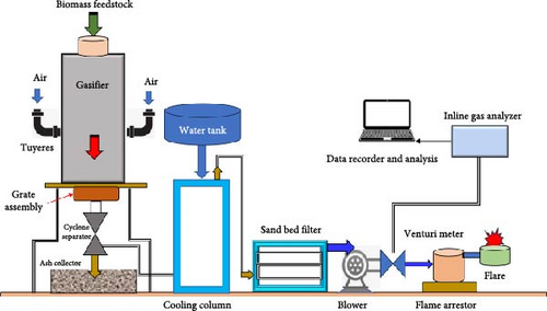
A fixed bed downdraft gasifier was employed in the study. It is made up of a cylindrical reactor with a fixed bed. A shakable and adjustable grate assembly is fitted for holding the biomass and effective ash removal at intervals. The air is supplied with the help of horizontal tuyeres fitted on the gasifier body. The bottom part of the reactor acts as the combustion zone, allowing for the controlled entry of extra air or oxygen. To survive the high temperatures created during the gasification process, the fixed bed is frequently made of heavy gauge steel plates. The biomass is supplied from the top side, and it moves downward during the process. A gas filter comprising three stages of sand beds was used for gas cleaning downstream of the grate assembly. A twin-column type cooling tower is employed for cooling down the producer gas. An inline gas analyzer is used to determine the hydrogen content in the ensuing PG. The composition of the PG was also used to estimate the lower heating values (LHV). The arrangement of the test setup is depicted in Figure 1.

Details are in the caption following the image — **Figure 1**
Open in figure viewer PowerPoint

Test setup depicting downdraft gasifier.

2.2. Biomass Feedstock

Waste mahua wood, derived from the mahua tree (Madhuca longifolia), has a lot of promise as a biomass feedstock for gasification operations. Mahua wood, which is widespread in tropical countries, particularly India, is noted for its high energy content and availability as a byproduct of numerous industries like mahua seed oil production [45, 46]. The thermochemical conversion of waste mahua wood into a combustible gas mixture is the mechanism by which waste mahua wood is gasified. Waste mahua wood has various favorable properties as a biomass fuel. First, its abundance as a byproduct assures a long-term and readily available supply for gasification, which contributes to waste utilization and sustainability of the environment. Second, mahua wood has a high energy content, making it an excellent option for efficient gasification procedures [45, 47, 48].

2.3. Machine Learning for Model Prediction

The present study makes use of two advanced ML techniques, i.e., AdaBoost and RF, for model prediction of LHV and hydrogen yield. The equivalence ratio (ER), gas flow rate (GFR), and residence time (RT) were employed as control factors in the present study. A range of these control factors were used to gather the data for modeling.

2.3.1. AdaBoost

In the case of ML-based regression, the endeavor is to predict continuous numerical values by making use of input characteristics. It has been observed that while conventional regression approaches provide reasonable predictions, their predictive performance drops in the case of nonlinear and complex data [49]. In these cases, ensemble-based approaches offer an efficient solution to increase the accuracy of forecast resilience. AdaBoost is one such efficient and robust ML techniques. It belongs to the family of adaptable ensemble learning approaches employed in the ML domain. It has a unique approach in which it makes use of its capacity to improve the performance of weak learners, also known as “base classifiers,” by applying variable weights to occurrences in the dataset based on classification accuracy. The basic foundation of AdaBoost regressor is its inherent approach of using iterative methods for training a base estimator or regression models, or estimators, in which each succeeding model concentrates on improving upon the errors or inaccuracies of its predecessors. AdaBoost regressor employs this approach of iterative improvement for successfully learning and comprehending the complex correlations inherent in the data, thus resulting in greater prognostic accuracy [50, 51].

The fundamentals of AdaBoost can be described as [52, 53, 54, 55]:

Let M be the number of base estimators in the case of regression models, and h_m(x) denotes the base estimator numbered as m_th, while the weight associated is shown with α_m.

In the case of the dataset containing input–output pairings

, where x_i are input characteristics and y_i are target values. The AdaBoostRegressor algorithm may be described as follows:

(1)
Initialize: Initialize the sample weight:

(1)

(2)
In the case of each iteration m = 1, 2, 3, …., M.

(i)
First, train a base estimator h_m(x) by employing the weighted dataset:
(2)
(ii)
Next, estimate the weighted error ∈_m for the m_th estimator, as follows:

(3)

(iii)
Now estimate the importance weight of m_th estimator:

(4)

(iv)
Next, update the sample weight:

; herein, Z_m is the factor of normalization which ensures that the total weighted sum is 1:
(5)
(3)
Then the final prediction is

(6)

This forms the basis for the AdaBoost regressor, in which each base estimator focuses on improving the preceding estimator, and then their predictions are combined with adaptive weights to form the final prediction. The success of AdaBoost in several fields is attributed to its ability to handle large datasets with resilience even in the case of complex and nonlinear data [54, 55].

2.3.2. RF

RF is another ML technique being employed in the present study for regression. RF belongs to the ensemble-based learning family. RF has emerged as a robust ML technique. RF is characterized by the development of an ensemble of individual decision trees (DTs), such that each DT is trained on a fraction of the data. During training, a random selection of characteristics is employed. This clever strategy gives each of the trees more diversity, leading to the creation of an ensemble model that excels in generalizing, precision, and robustness [56, 57]. RF does have the robust efficiency to reduce the chances of overfitting, a common challenge with conventional DTs by combining forecasts from many trees. In light of this, RF excels at managing high-dimensional data and complex variable relationships [58, 59].

It can be summarized as follows [52, 53, 57, 58]:

In this case, N denotes the sample count in a given dataset, if D is the number of input features, while X is the input feature matrix N × D, and y is the target variable vector of N × 1. RF-based regression approach creates a set of DTs T₁, T₂, T₃, …, T_M where M is the number of trees in the forest. Here, T_M DT was trained on a bootstrapped sample, and it employs a randomly selected subset of characteristics at each node.

To predict

from a fresh input feature vector x, the RF-based regression model averages the predictions of all discrete trees:

(7)

The forecast by m_th DT for the input feature vector x is represented by T_m(x). The T_m DT predicts the target variable employing the binary splits in the feature space. The split at each node of the tree is based on the arbitrarily chosen feature subset and reduces target variable variation within each subset. The RF-based regression model predicts the target variable robustly by using mean predictions of all trees. This strategy helps even in case of even the case of nonlinear as well as noisy data [60, 61].

2.3.3. LR

The LR method is a fundamental ML technique that is employed for forecasting the numerical values on the basis of the data that are supplied. Additionally, it presupposes that there is a linear relationship between the characteristics and the variable of interest. Through the process of learning the coefficients that provide the greatest match to the data, the model can generate forecasts for new inputs. Forecasting, analysis of trends, and correlation discovery are just some of the numerous sectors that make extensive use of this tool. LR is also an effective approach for creating a baseline prediction model in the case when multiple models are being tested. The use of LR as a baseline prediction model makes it easier to evaluate the increased predictive power achieved by rather complex ML algorithms. LR has its strength, specifically in cases when data depict a linear trend [62, 63]. On the other hand,it has limits in the case when dealing with complex and nonlinear data patterns. There are certain circumstances in which more complicated models, like DTs or ANN, may perform better than LR. The contrast between the simplicity of LR to these many advanced models sheds light on the tradeoff that exists between the level of complexity of the model and the precision of the forecast.

2.4. Model Evaluation

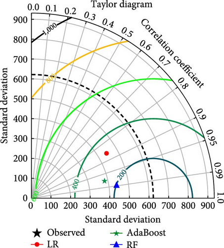
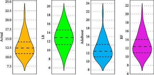
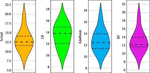
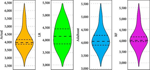
In the present study, several approaches to evaluating the prediction models developed in the present study were employed to ensure that a robust comparison can be made. Two different approaches were employed; firstly, numerical methods like the coefficient of determinations (R²), mean absolute percentage errors (MAPE), and root mean squared errors (RMSE) were employed [64, 65]. Also, a twin-pronged approach of Taylor’s diagrams as well as violin plots was employed in the study. The use of Taylor’s diagrams is an efficient and easy-to-use graphical tool to estimate the efficacy of ML models, specifically when several ML-based models to compared. The proximity of nodes to the benchmark standard, the correlation coefficient, and the RMSE ratio all provide information about the models’ dependability and correctness [66, 67]. Violin plots integrate the characteristics of kernel density plots as well as box plots. A violin plot combines model categories with prediction distributions. For each model category, quartiles, as well as median lines, offer a summary comparison of the model’s central tendencies and dispersion [68].

3. Results and Discussion

The data was collected from extensive testing of the biomass gasification process from waste mahua wood. Different settings of ER, RT, and GFR were used and response variables; namely, hydrogen yield and LHV were recorded. This data was then used for model development. Seventy percent of the experimental data was used to train the models, while the remaining 30% was employed for testing the models.

3.1. Data Analysis

The correlation heatmap (Figure 2(a)) and descriptive statistical analysis, as well as the violin plots (Figure 2(b)), were employed for data analysis to evaluate the correlations among data columns. A high correlation between ER and hydrogen yield of 0.61 was observed indicating a strong positive link between these two. The correlation between ER and hydrogen production was 0.5, indicating a somewhat lower degree of correlation between the two compared to ER and hydrogen production. On the other hand, it was observed that the correlation between GFR and hydrogen yield was negative at −0.38, indicating that higher gas flow out of the gasifier negatively impacts the hydrogen yields.

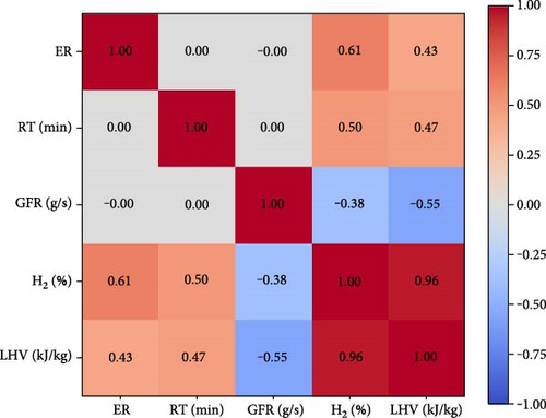
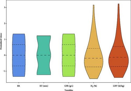
In the case of a correlation between LHV and control factors, it was observed that the correlation value between ER and LHV was 0.43, while it was 0.47 between RT and LHV indicating a comparable positive link between these parameters. In the case of GFR and LHV, a negative correlation of −0.55 was observed, indicating that a higher rate of GFR reduces the LHV of outgoing PG. The violin plots depict the concentrations and dispersion of the data of different parameters.

3.2. Hydrogen Yield Models

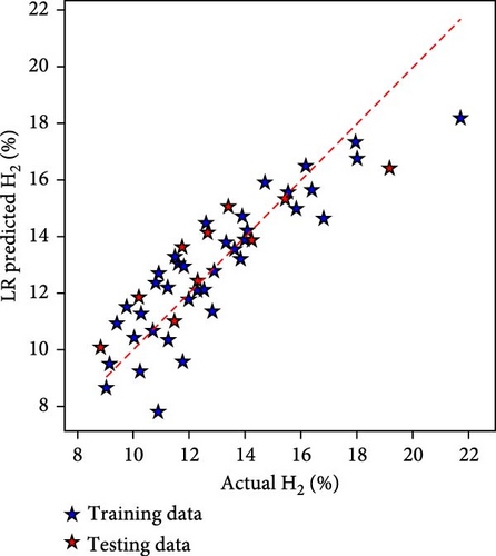
The hydrogen content in the producer gas is the most significant element as it directly impacts the quality and heating value of PG. Hence, it was considered for model predictions. Figure 3 depicts the performance of all three ML techniques employed in the present study in the model form of actual vs. model prediction. Figure 3(a) depicts the LR-based model, and Figure 3(b) shows the AdaBoost-based model, while Figure 3(c) depicts the RF-based hydrogen yield model. The closeness of the data points to diagonal lines shows the robustness of the models. It can be observed that the RF-based hydrogen yield model performs superior to the other two models.

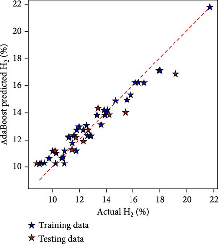
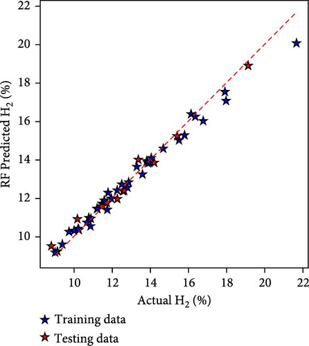
The models were also evaluated based on statistical metrics. The statistical evaluation of the models has been listed in Table 2. During the model training phase, RF has the lowest MSE of 0.17, followed by AdaBoost with 0.405 and LR with 1.717. On the R² metric, RF surpasses AdaBoost and LR, with a score of 0.978 vs. 0.948 and 0.779, respectively. The MAE demonstrates RF’s superior performance, with a value of 0.29 compared to AdaBoost’s 0.527 and LR 1.012. These indicators reflect the models’ capacity to produce correct predictions, with RF consistently outperforming other models in this specific modeling environment in terms of precision as well as low errors.

Table 2. Statistical evaluation of models.

	Training/testing	Metric	LR	AdaBoost	RF
H₂ model	Training	Mean squared error	1.717	0.405	0.17
		R²	0.779	0.948	0.978
		Mean absolute error	1.012	0.527	0.29
		Explained variance	0.779	0.95	0.979
	Testing	Mean squared error	2.106	1.193	0.181
		R²	0.721	0.842	0.976
		Mean absolute error	1.183	0.857	0.357
		Explained variance	0.751	0.844	0.976

LHV model	Training	Mean squared error	100,933	24,612.55	8,297.74
		R²	0.713	0.93	0.977
		Mean absolute error	243.715	134.01	70.07
		Explained variance	0.7131	0.937	0.977
	Testing	Mean squared error	110,086.2	71,800.02	11,350.04
		R²	0.715	0.814	0.971
		Mean absolute error	259.03	198.6	93
		Explained variance	0.718	0.815	0.972

On the other hand, during model testing using 30% fresh data, when looking at the MSE, the results show that RF works better than both LR and AdaBoost, with an MSE value of 0.181. AdaBoost comes in second with an MSE of 1.192, and LR comes in third with an MSE of 2.106. With a score of 0.976, the R² number, which measures how well the models fit, shows that the RF model is the best, beating out AdaBoost (0.842) and LR (0.721). Furthermore, RF has a lower MAE value of 0.357 compared to AdaBoost’s 0.857 and LR’s 1.183, making it the best. The trend of explained variance is also the same, with RF getting a score of 0.976, which is higher than both AdaBoost (0.844) and LR (0.751). All of these data show that RF is better at predicting what will happen in this modeling case.

3.3. LHV Models

The LHV denotes the lower heating value of the producer gas in this study. Figure 4 depicts the performance of all three ML techniques employed in the present study for the model prediction of LHV data. Figure 4(a) shows the outcome of the LR-based model, and Figure 4(b) depicts the AdaBoost-based model, while Figure 4(c) depicts the RF-based LHV model. The proximity of the data points to diagonal lines demonstrates the models’ resilience. The RF-based LHV model outperforms the other two models as it can be observed that most of the data points lie close to the diagonal line.

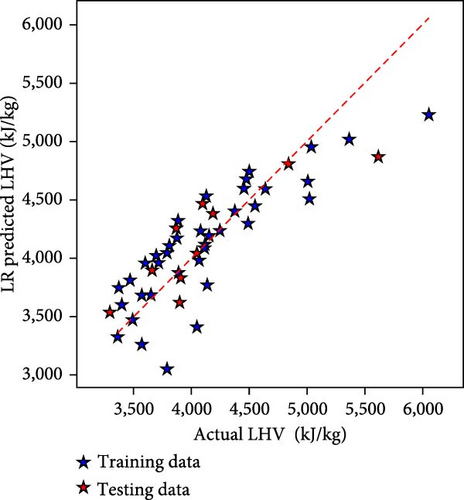
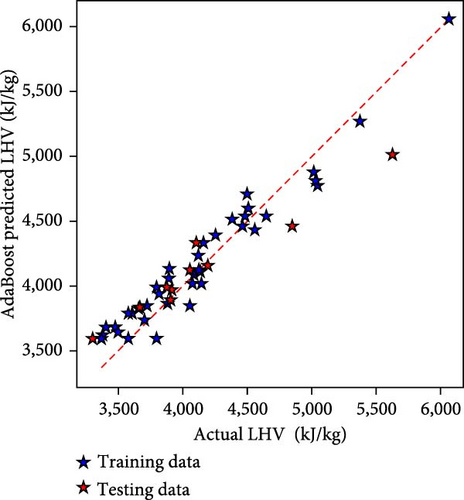
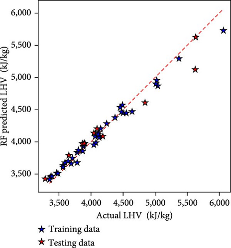
These prediction models were developed with LR, RF, and AdaBoost and then combined with statistical methods. Table 2 lists the performance metrics for ML models. During the model training phase, in terms of MSE, the figures show substantial variances, with RF having the lowest error at 8,297.74, AdaBoost having 24,612.55, and LR having 100,933. With a score of 0.976, RF outperforms AdaBoost at 0.93 and LR at 0.713 in the R² metric, which estimates goodness of fit. MAE highlights the RF’s precision even more, with the lowest value of 70.07, followed by AdaBoost at 134.01 and LR at 243.72. These patterns are mirrored in explained variance, with RF leading at 0.977, AdaBoost at 0.937, and LR at 0.713. In this scenario, these criteria jointly identify RF as the most successful model in terms of accuracy and predictive performance.

In the model testing phase also, RF has the lowest MSE at 11,350.04, surpassing AdaBoost at 71,800.02 and LR at 110,086.2. RF has the greatest R² score of 0.971, topping AdaBoost at 0.814 and LR at 0.715, representing the quality of fit. Furthermore, RF outperforms both AdaBoost and LR in terms of MAE, with low values of 93 and 259.03, correspondingly. With a score of 0.972, the explained variance measure confirms RF’s better performance over AdaBoost and LR. These metrics highlight the RF-based model’s efficacy in generating higher accuracy and better model fit.

3.4. Model Comparison

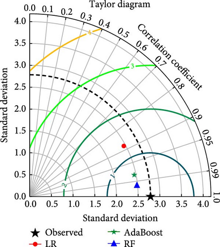
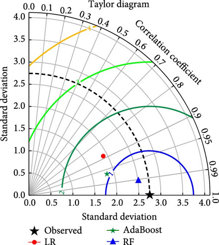
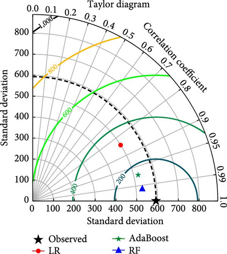
The models developed with LR, RF, and AdaBosst were also compared with advanced methods of Taylor’s diagram and violin plots. Figure 5(a) depicts Taylor’s diagram for model comparison during model training, while Figure 5(b) depicts Taylor’s diagram during model testing in the case of hydrogen yield models. Also, Figure 6(a) depicts Taylor’s diagram for model comparison during model training, while Figure 6(b) depicts Taylor’s diagram during model testing in the case of LHV models. Taylor’s diagrams also show the superiority of RF-based models for both hydrogen yield and LHV models. The models were also compared with violin plots as it is easy to identify the superior models with this approach. The violin plots of the model having almost mirror reflection are considered superior since it is almost similar to actual data. Figures 7(a) and 7(b) depict the violin plots for hydrogen yield models during model training as well as model testing, respectively. Figures 8(a) and 8(b) depict the violin plots for LHV models during model training as well as model testing, respectively. In this also, it can be observed that violin plots are almost similarly shaped as actual data violin plots. This indicates excellent performance and low error in the case of RF-based models.

4. Conclusions

In the present study, waste mahua biomass was used for the generation of producer gas. The effects of control factors like equivalence ratio, residence time, and gas flow rate on response variables like hydrogen yield and LHV value of producer gas were investigated. The data gathered through experimental work were employed for model prediction. Two recent but highly efficient ML approaches, RF and AdaBoost, were employed. The outcomes were used in conjunction with the results of a baseline approach, namely, LR. The main outcomes of the study are listed as follows:

(1)
RF outperformed AdaBoost (0.4048) and LR (1.717) in the hydrogen yield prediction model during training, delivering the lowest MSE at 0.17.
(2)
RF outperformed AdaBoost (24612.55) and LR (100933) in LHV models during training, with the lowest MSE of 8297.74, reaffirming its accuracy in forecasting LHV.
(3)
RF maintained its lead in hydrogen yield model testing, with the lowest MSE of 0.181, topping AdaBoost (1.193) and LR (2.106).
(4)
Taylor’s diagrams and violin plots repeatedly demonstrated RF’s superiority, validating its ability to forecast hydrogen yield and LHV properly in both training and testing.

ML techniques like RF and AdaBoost are useful tools for simulating biomass gasification, but their efficacy depends upon the data quality. Another issue is that the prediction model’s employability to various biomass types is restricted owing to differences in biomass properties. On the other hand, the ML-based strategies may enhance the process efficiency by properly anticipating critical factors like the control factors and response variables. The robust prognostic models for biomass gasification may assist stakeholders in energy sector stakeholders in making informed choices like assessing biomass gasification viability for any project and technical improvement.

Abbreviations

AdaBoost:: Adaptive boosting
ANN:: Artificial neural networks
BTE:: Brake thermal efficiency
CO:: Carbon monoxide
CO₂:: Carbon dioxide
DF:: Dual-fuel
ER:: Equivalence ratio
GFR:: Gas flow rate
GHG:: Greenhouse gases
H₂:: Hydrogen
kWe:: Kilowatts electrical
LR:: Linear regression
MSE:: Mean squared error
ML:: Machine learning
MAPE:: Mean absolute percentage error
MAE:: Mean absolute error
NARX:: Nonlinear autoregressive with exogenous inputs
PG:: Producer gas
R²:: Coefficient of determinations
RDF:: Refuse driven fuel
RF:: Random forest
RMSE:: Root mean squared error
RT:: Residence time
SDGs:: Sustainable development goals
w/w:: Weights/weights
LHV:: Lower heating value.

Conflicts of Interest

The authors declare that they have no conflicts of interest

Authors’ Contributions

Mansoor Alruqi is responsible for the conceptualization, methodology, data curation, and writing, original draft. P. Sharma is responsible for the writing, review and editing, resources, and supervision. Prabhu Paramasivam is responsible for the writing, original draft, and writing, review and editing. H. A. Hanafi is responsible for the methodology, writing, review and editing, and supervision.

Acknowledgments

The author (Mansoor Alruqi) would like to thank the Deanship of Scientific Research at Shaqra University for supporting this work.

Open Research

Data Availability

Data available on request.

References

1 Mayer F. D., Brondani M., Vasquez Carrillo M. C., Hoffmann R., and Lora E. E. S., Revisiting energy efficiency, renewability, and sustainability indicators in biofuels life cycle: analysis and standardization proposal, Journal of Cleaner Production. (2020) 252, https://doi.org/10.1016/j.jclepro.2019.119850, 119850.
10.1016/j.jclepro.2019.119850
Web of Science® Google Scholar
2 Alola A. A., Abbas S., and Alola U. V., Examining the effect of global energy reserves to production ratio on carbon emission in the USA, Energy Strategy Reviews. (2024) 52, https://doi.org/10.1016/j.esr.2024.101353, 101353.
10.1016/j.esr.2024.101353
Web of Science® Google Scholar
3 Abuadala A. and Dincer I., A review on biomass-based hydrogen production and potential applications, International Journal of Energy Research. (2012) 36, no. 4, 415–455, https://doi.org/10.1002/er.1939, 2-s2.0-84858863532.
10.1002/er.1939
CAS Web of Science® Google Scholar
4 Vamvuka D., Bio-oil, solid and gaseous biofuels from biomass pyrolysis processes—an overview, International Journal of Energy Research. (2011) 35, no. 10, 835–862, https://doi.org/10.1002/er.1804, 2-s2.0-79960351376.
10.1002/er.1804
CAS Web of Science® Google Scholar
5 Han J., Yao X., Zhan Y., Oh S.-Y., Kim L.-H., and Kim H.-J., A method for estimating higher heating value of biomass-plastic fuel, Journal of the Energy Institute. (2017) 90, no. 2, 331–335, https://doi.org/10.1016/j.joei.2016.01.001, 2-s2.0-85020657134.
10.1016/j.joei.2016.01.001
CAS Web of Science® Google Scholar
6 khan M., Raza Naqvi S., Ullah Z., Ali Ammar Taqvi S., Nouman Aslam Khan M., Farooq W., Taqi Mehran M., Juchelková D., and Štěpanec L., Applications of machine learning in thermochemical conversion of biomass—a review, Fuel. (2023) 332, https://doi.org/10.1016/j.fuel.2022.126055, 126055.
10.1016/j.fuel.2022.126055
CAS Web of Science® Google Scholar
7 Yu M., Kubiczek J., Ding K., Jahanzeb A., and Iqbal N., Revisiting SDG-7 under energy efficiency vision 2050: the role of new economic models and mass digitalization in OECD, Energy Efficiency. (2022) 15, no. 1, https://doi.org/10.1007/s12053-021-10010-z.
10.1007/s12053-021-10010-z
PubMed Web of Science® Google Scholar
8 IEA, IRENA, UNSD, and Bank W., WHO: Tracking SDG7: The Eneergy Progress Report 2022, 2022, World Bank.
Google Scholar
9 Thapa P., Mainali B., and Dhakal S., Focus on climate action: what level of synergy and trade-off is there between SDG 13; climate action and other SDGs in Nepal?, Energies. (2023) 16, no. 1, https://doi.org/10.3390/en16010566, 566.
10.3390/en16010566
Google Scholar
10 Beccarello M. and Di Foggia G., Sustainable development goals data-driven local policy: focus on SDG 11 and SDG 12, Administrative Sciences. (2022) 12, no. 4, https://doi.org/10.3390/admsci12040167, 167.
10.3390/admsci12040167
Web of Science® Google Scholar
11 Chen W.-H., Hoang A. T., Nižetić S., Pandey A., Cheng C. K., Luque R., Ong H. C., Thomas S., and Nguyen X. P., Biomass-derived biochar: from production to application in removing heavy metal-contaminated water, Process Safety and Environmental Protection. (2022) 160, 704–733, https://doi.org/10.1016/j.psep.2022.02.061.
10.1016/j.psep.2022.02.061
CAS Web of Science® Google Scholar
12 Hoang A. T., Ong H. C., Fattah I. M. R., Chong C. T., Cheng C. K., Sakthivel R., and Ok Y. S., Progress on the lignocellulosic biomass pyrolysis for biofuel production toward environmental sustainability, Fuel Processing Technology. (2021) 223, https://doi.org/10.1016/j.fuproc.2021.106997, 106997.
10.1016/j.fuproc.2021.106997
CAS Web of Science® Google Scholar
13 Burke M. J. and Melgar R., SDG 7 requires post-growth energy sufficiency, Frontiers in Sustainability. (2022) 3, https://doi.org/10.3389/frsus.2022.940958.
10.3389/frsus.2022.940958
Web of Science® Google Scholar
14 Hoang A. T., Pham V. V., and Nguyen X. P., Integrating renewable sources into energy system for smart city as a sagacious strategy towards clean and sustainable process, Journal of Cleaner Production. (2021) 305, https://doi.org/10.1016/j.jclepro.2021.127161, 127161.
10.1016/j.jclepro.2021.127161
Web of Science® Google Scholar
15 Kalinci Y., Hepbasli A., and Dincer I., Biomass-based hydrogen production: a review and analysis, International Journal of Hydrogen Energy. (2009) 34, no. 21, 8799–8817, https://doi.org/10.1016/j.ijhydene.2009.08.078, 2-s2.0-71549143842.
10.1016/j.ijhydene.2009.08.078
CAS Web of Science® Google Scholar
16 Wang Y., Cai C., Liu C., Han X., and Zhou M., Planning research on rural integrated energy system based on coupled utilization of biomass-solar energy resources, Sustainable Energy Technologies and Assessments. (2022) 53, https://doi.org/10.1016/j.seta.2022.102416, 102416.
10.1016/j.seta.2022.102416
Web of Science® Google Scholar
17 Shafizadeh A., Shahbeik H., Rafiee S., Moradi A., Shahbaz M., Madadi M., Li C., Peng W., Tabatabaei M., and Aghbashlo M., Machine learning-based characterization of hydrochar from biomass: implications for sustainable energy and material production, Fuel. (2023) 347, https://doi.org/10.1016/j.fuel.2023.128467, 128467.
10.1016/j.fuel.2023.128467
CAS Web of Science® Google Scholar
18 Shahbeik H., Rafiee S., Shafizadeh A., Jeddi D., Jafary T., Lam S. S., Pan J., Tabatabaei M., and Aghbashlo M., Characterizing sludge pyrolysis by machine learning: towards sustainable bioenergy production from wastes, Renewable Energy. (2022) 199, 1078–1092, https://doi.org/10.1016/j.renene.2022.09.022.
10.1016/j.renene.2022.09.022
Web of Science® Google Scholar
19 Kumar B. and Verma P., Biomass-based biorefineries: an important architype towards a circular economy, Fuel. (2021) 288, https://doi.org/10.1016/j.fuel.2020.119622, 119622.
10.1016/j.fuel.2020.119622
CAS Web of Science® Google Scholar
20 Umar M., Ji X., Kirikkaleli D., and Alola A. A., The imperativeness of environmental quality in the United States transportation sector amidst biomass-fossil energy consumption and growth, Journal of Cleaner Production. (2021) 285, https://doi.org/10.1016/j.jclepro.2020.124863, 124863.
10.1016/j.jclepro.2020.124863
CAS Web of Science® Google Scholar
21 Sharma P. and Sharma A. K., Statistical and continuous wavelet transformation-based analysis of combustion instabilities in a biodiesel-fueled compression ignition engine, Journal of Energy Resources Technology. (2022) 144, no. 3, https://doi.org/10.1115/1.4051340.
10.1115/1.4051340
Web of Science® Google Scholar
22 Susastriawan A. A. P., Saptoadi H., and Purnomo, Small-scale downdraft gasifiers for biomass gasification: a review, Renewable and Sustainable Energy Reviews. (2017) 76, 989–1003, https://doi.org/10.1016/j.rser.2017.03.112, 2-s2.0-85016292362.
10.1016/j.rser.2017.03.112
CAS Web of Science® Google Scholar
23 Halewadimath S. S., Banapurmath N. R., Yaliwal V. S., Gaitonde V. N., Khan T. M. Y., Vadlamudi C., Krishnappa S., and Sajjan A. M., Experimental investigations on dual-fuel engine fueled with tertiary renewable fuel combinations of biodiesel and producer—hydrogen gas using response surface methodology, Sustainability. (2023) 15, no. 5, https://doi.org/10.3390/su15054483, 4483.
10.3390/su15054483
CAS Web of Science® Google Scholar
24 Dabi M. and Saha U. K., Experimental analysis of a dual-fuel engine fueled by producer gas derived from pine leaves and cattle dung briquettes, ASME. 2015 Gas Turbine India Conference. (2015) https://doi.org/10.1115/GTINDIA2015-1263, 2-s2.0-84964394233, V001T11A002.
10.1115/GTINDIA2015-1263
Google Scholar
25 Safarian S., Unnthorsson R., and Richter C., Performance analysis and environmental assessment of small-scale waste biomass gasification integrated CHP in Iceland, Energy. (2020) 197, https://doi.org/10.1016/j.energy.2020.117268, 117268.
10.1016/j.energy.2020.117268
CAS Web of Science® Google Scholar
26 Nobre C., Longo A., Vilarinho C., and Gonçalves M., Gasification of pellets produced from blends of biomass wastes and refuse derived fuel chars, Renewable Energy. (2020) 154, 1294–1303, https://doi.org/10.1016/j.renene.2020.03.077.
10.1016/j.renene.2020.03.077
CAS Web of Science® Google Scholar
27 Nagy G. and Dobó Z., Experimental investigation of fixed-bed pyrolysis and steam gasification of food waste blended with woody biomass, Biomass and Bioenergy. (2020) 139, https://doi.org/10.1016/j.biombioe.2020.105580, 105580.
10.1016/j.biombioe.2020.105580
CAS Web of Science® Google Scholar
28 Cai J., Zeng R., Zheng W., Wang S., Han J., Li K., Luo M., and Tang X., Synergistic effects of co-gasification of municipal solid waste and biomass in fixed-bed gasifier, Process Safety and Environmental Protection. (2021) 148, 1–12, https://doi.org/10.1016/j.psep.2020.09.063.
10.1016/j.psep.2020.09.063
CAS Web of Science® Google Scholar
29 Li J., Xu K., Yao X., and Chen S., Prediction and optimization of syngas production from steam gasification: numerical study of operating conditions and biomass composition, Energy Conversion and Management. (2021) 236, https://doi.org/10.1016/j.enconman.2021.114077, 114077.
10.1016/j.enconman.2021.114077
CAS Web of Science® Google Scholar
30 Buentello-Montoya D. A., Duarte-Ruiz C. A., and Maldonado-Escalante J. F., Co-gasification of waste PET, PP and biomass for energy recovery: a thermodynamic model to assess the produced syngas quality, Energy. (2023) 266, https://doi.org/10.1016/j.energy.2022.126510, 126510.
10.1016/j.energy.2022.126510
CAS Web of Science® Google Scholar
31 Salavati S., Zhang C. T., Zhang S., Liu Q., Gholizadeh M., and Hu X., Cross-interaction during co-gasification of wood, weed, plastic, tire and carton, Journal of Environmental Management. (2019) 250, https://doi.org/10.1016/j.jenvman.2019.109467, 2-s2.0-85071292535, 109467.
10.1016/j.jenvman.2019.109467
CAS PubMed Web of Science® Google Scholar
32 Fazil A., Kumar S., and Mahajani S. M., Gasification and co-gasification of paper-rich, high-ash refuse-derived fuel in downdraft gasifier, Energy. (2023) 263, https://doi.org/10.1016/j.energy.2022.125659, 125659.
10.1016/j.energy.2022.125659
CAS Web of Science® Google Scholar
33 Awais M., Omar M. M., Munir A., li W., Ajmal M., Hussain S., Ahmad S. A., and Ali A., Co-gasification of different biomass feedstock in a pilot-scale (24 kWe) downdraft gasifier: an experimental approach, Energy. (2022) 238, https://doi.org/10.1016/j.energy.2021.121821, 121821.
10.1016/j.energy.2021.121821
CAS Web of Science® Google Scholar
34 Li H., Chen J., Zhang W., Zhan H., He C., Yang Z., Peng H., and Leng L., Machine-learning-aided thermochemical treatment of biomass: a review, Biofuel Research Journal. (2023) 10, no. 1, 1786–1809, https://doi.org/10.18331/BRJ2023.10.1.4.
10.18331/BRJ2023.10.1.4
CAS Web of Science® Google Scholar
35 Wang H. S.-H. and Yao Y., Machine learning for sustainable development and applications of biomass and biomass-derived carbonaceous materials in water and agricultural systems: a review, Resources, Conservation and Recycling. (2023) 190, https://doi.org/10.1016/j.resconrec.2022.106847, 106847.
10.1016/j.resconrec.2022.106847
Web of Science® Google Scholar
36 Hu G. and You F., Renewable energy-powered semi-closed greenhouse for sustainable crop production using model predictive control and machine learning for energy management, Renewable and Sustainable Energy Reviews. (2022) 168, https://doi.org/10.1016/j.rser.2022.112790, 112790.
10.1016/j.rser.2022.112790
Web of Science® Google Scholar
37 Goettsch D., Castillo-Villar K. K., and Aranguren M., Machine-learning methods to select potential depot locations for the supply chain of biomass co-firing, Energies. (2020) 13, no. 24, https://doi.org/10.3390/en13246554, 6554.
10.3390/en13246554
CAS Web of Science® Google Scholar
38 Zhang W., Chen Q., Chen J., Xu D., Zhan H., Peng H., Pan J., Vlaskin M., Leng L., and Li H., Machine learning for hydrothermal treatment of biomass: a review, Bioresource Technology. (2023) 370, https://doi.org/10.1016/j.biortech.2022.128547, 128547.
10.1016/j.biortech.2022.128547
CAS PubMed Web of Science® Google Scholar
39 Sahoo D. and Remya N., Influence of operating parameters on the microwave pyrolysis of rice husk: biochar yield, energy yield, and property of biochar, Biomass Conversion and Biorefinery. (2022) 12, no. 8, 3447–3456, https://doi.org/10.1007/s13399-020-00914-8.
10.1007/s13399-020-00914-8
CAS Web of Science® Google Scholar
40 Veza I., Afzal A., Mujtaba M. A., Tuan Hoang A., Balasubramanian D., Sekar M., Fattah I. M. R., Soudagar M. E. M., EL-Seesy A. I., Djamari D. W., Hananto A. L., Putra N. R., and Tamaldin N., Review of artificial neural networks for gasoline, diesel and homogeneous charge compression ignition engine: review of ANN for gasoline, diesel and HCCI engine, Alexandria Engineering Journal. (2022) 61, no. 11, 8363–8391, https://doi.org/10.1016/j.aej.2022.01.072.
10.1016/j.aej.2022.01.072
Web of Science® Google Scholar
41 Yucel O., Aydin E. S., and Sadikoglu H., Comparison of the different artificial neural networks in prediction of biomass gasification products, International Journal of Energy Research. (2019) 43, no. 11, 5992–6003, https://doi.org/10.1002/er.4682, 2-s2.0-85068529998.
10.1002/er.4682
CAS Web of Science® Google Scholar
42 Leng L., Yang L., Lei X., Zhang W., Ai Z., Yang Z., Zhan H., Yang J., Yuan X., Peng H., and Li H., Machine learning predicting and engineering the yield, N content, and specific surface area of biochar derived from pyrolysis of biomass, Biochar. (2022) 4, no. 1, https://doi.org/10.1007/s42773-022-00183-w, 63.
10.1007/s42773-022-00183-w
CAS Web of Science® Google Scholar
43 Kargbo H. O., Zhang J., and Phan A. N., Optimisation of two-stage biomass gasification for hydrogen production via artificial neural network, Applied Energy. (2021) 302, https://doi.org/10.1016/j.apenergy.2021.117567, 117567.
10.1016/j.apenergy.2021.117567
CAS Web of Science® Google Scholar
44 Cerinski D., Baleta J., Mikulčić H., Mikulandrić R., and Wang J., Dynamic modelling of the biomass gasification process in a fixed bed reactor by using the artificial neural network, Cleaner Engineering and Technology. (2020) 1, https://doi.org/10.1016/j.clet.2020.100029, 100029.
10.1016/j.clet.2020.100029
Web of Science® Google Scholar
45 Gupta A., Chaudhary R., and Sharma S., Potential applications of mahua (Madhuca indica) biomass, Waste and Biomass Valorization. (2012) 3, no. 2, 175–189, https://doi.org/10.1007/s12649-012-9107-9, 2-s2.0-84863688695.
10.1007/s12649-012-9107-9
Web of Science® Google Scholar
46 Raj R., Kumar Singh D., and Tirkey J. V., Co-gasification of Low-grade coal with Madhuca longifolia (Mahua) biomass and dual-fuelled mode engine performance: effect of biomass blend and engine operating condition, Energy Conversion and Management. (2022) 269, https://doi.org/10.1016/j.enconman.2022.116150, 116150.
10.1016/j.enconman.2022.116150
CAS Web of Science® Google Scholar
47 Puhan S., Vedaraman N., Sankaranarayanan G., Bharat Ram B. V., and Jeychandran K., Mahua oil (Madhuca Indica seed oil) methyl ester as biodiesel-preparation and emission characteristics, Biomass and Bioenergy. (2005) 28, no. 1, 87–93, https://doi.org/10.1016/j.biombioe.2004.06.002, 2-s2.0-7444246779.
10.1016/j.biombioe.2004.06.002
CAS Web of Science® Google Scholar
48 Dhanavath K. N., Bankupalli S., Bhargava S. K., and Parthasarathy R., An experimental study to investigate the effect of torrefaction temperature on the kinetics of gas generation, Journal of Environmental Chemical Engineering. (2018) 6, no. 2, 3332–3341, https://doi.org/10.1016/j.jece.2018.05.016, 2-s2.0-85047016531.
10.1016/j.jece.2018.05.016
CAS Web of Science® Google Scholar
49 Gupta K. K., Kalita K., Ghadai R. K., Ramachandran M., and Gao X. Z., Machine learning-based predictive modelling of biodiesel production—a comparative perspective, Energies. (2021) 14, no. 4, https://doi.org/10.3390/en14041122, 1122.
10.3390/en14041122
CAS Web of Science® Google Scholar
50 Busari G. A. and Lim D. H., Crude oil price prediction: a comparison between AdaBoost-LSTM and AdaBoost-GRU for improving forecasting performance, Computers & Chemical Engineering. (2021) 155, https://doi.org/10.1016/j.compchemeng.2021.107513, 107513.
10.1016/j.compchemeng.2021.107513
CAS Web of Science® Google Scholar
51 Li R., Sun H., Wei X., Ta W., and Wang H., Lithium battery state-of-charge estimation based on AdaBoost.Rt-RNN, Energies. (2022) 15, no. 16, https://doi.org/10.3390/en15166056, 6056.
10.3390/en15166056
CAS Web of Science® Google Scholar
52 Breiman L., Random forests, Machine Learning. (2001) 45, no. 1, 5–32, https://doi.org/10.1023/A:1010933404324, 2-s2.0-0035478854.
10.1023/A:1010933404324
Web of Science® Google Scholar
53 Biau G. and Scornet E., A random forest guided tour, TEST. (2016) 25, no. 2, 197–227, https://doi.org/10.1007/s11749-016-0481-7, 2-s2.0-84964330838.
10.1007/s11749-016-0481-7
Web of Science® Google Scholar
54 Liu B., Liu C., Xiao Y., Liu L., Li W., and Chen X., AdaBoost-based transfer learning method for positive and unlabelled learning problem, Knowledge-Based Systems. (2022) 241, https://doi.org/10.1016/j.knosys.2022.108162, 108162.
10.1016/j.knosys.2022.108162
Web of Science® Google Scholar
55 Shahraki A., Abbasi M., and Haugen Ø., Boosting algorithms for network intrusion detection: a comparative evaluation of Real AdaBoost, Gentle AdaBoost and Modest AdaBoost, Engineering Applications of Artificial Intelligence. (2020) 94, https://doi.org/10.1016/j.engappai.2020.103770, 103770.
10.1016/j.engappai.2020.103770
Web of Science® Google Scholar
56 Walker A. M., Cliff A., Romero J., Shah M. B., Jones P., Felipe Machado Gazolla J. G., Jacobson D. A., and Kainer D., Evaluating the performance of random forest and iterative random forest based methods when applied to gene expression data, Computational and Structural Biotechnology Journal. (2022) 20, 3372–3386, https://doi.org/10.1016/j.csbj.2022.06.037.
10.1016/j.csbj.2022.06.037
CAS PubMed Web of Science® Google Scholar
57 Schonlau M. and Zou R. Y., The random forest algorithm for statistical learning, The Stata Journal: Promoting communications on statistics and Stata. (2020) 20, no. 1, 3–29, https://doi.org/10.1177/1536867X20909688.
10.1177/1536867X20909688
Google Scholar
58 Speiser J. L., Miller M. E., Tooze J., and Ip E., A comparison of random forest variable selection methods for classification prediction modeling, Expert Systems with Applications. (2019) 134, 93–101, https://doi.org/10.1016/j.eswa.2019.05.028, 2-s2.0-85066732412.
10.1016/j.eswa.2019.05.028
PubMed Web of Science® Google Scholar
59 Mohammadi M., Khorrami M. K., and Ghasemzadeh H., Classification of nanofluids solutions based on viscosity values: A comparative study of random forest, logistic model tree, Bayesian network, and support vector machine models, Infrared Physics & Technology. (2022) 125, https://doi.org/10.1016/j.infrared.2022.104273, 104273.
10.1016/j.infrared.2022.104273
Web of Science® Google Scholar
60 Shanmugasundar G., Vanitha M., Čep R., Kumar V., Kalita K., and Ramachandran M., A comparative study of linear, random forest and adaboost regressions for modeling non-traditional machining, Processes. (2021) 9, no. 11, https://doi.org/10.3390/pr9112015, 2015.
10.3390/pr9112015
CAS Web of Science® Google Scholar
61 N. G., Jain P., Choudhury A., Dutta P., Kalita K., and Barsocchi P., Random forest regression-based machine learning model for accurate estimation of fluid flow in curved pipes, Processes. (2021) 9, no. 11, https://doi.org/10.3390/pr9112095, 2095.
10.3390/pr9112095
CAS Google Scholar
62 Maulud D. and Abdulazeez A. M., A review on linear regression comprehensive in machine learning, Journal of Applied Science and Technology Trends. (2020) 1, no. 2, 140–147, https://doi.org/10.38094/jastt1457.
10.38094/jastt1457
Google Scholar
63 Öztürk O. B. and Başar E., Multiple linear regression analysis and artificial neural networks based decision support system for energy efficiency in shipping, Ocean Engineering. (2022) 243, https://doi.org/10.1016/j.oceaneng.2021.110209, 110209.
10.1016/j.oceaneng.2021.110209
Web of Science® Google Scholar
64 Gopi A., Sharma P., Sudhakar K., Ngui W. K., Kirpichnikova I., and Cuce E., Weather impact on solar farm performance: a comparative analysis of machine learning techniques, Sustainability. (2023) 15, no. 1, https://doi.org/10.3390/su15010439, 439.
10.3390/su15010439
Web of Science® Google Scholar
65 Alruqi M. and Sharma P., Biomethane production from the mixture of sugarcane vinasse, solid waste and spent tea waste: a bayesian approach for hyperparameter optimization for gaussian process regression, Fermentation. (2023) 9, no. 2, https://doi.org/10.3390/fermentation9020120, 120.
10.3390/fermentation9020120
CAS Web of Science® Google Scholar
66 Taylor K. E., Summarizing multiple aspects of model performance in a single diagram, Journal of Geophysical Research: Atmospheres. (2001) 106, no. D7, 7183–7192, https://doi.org/10.1029/2000JD900719, 2-s2.0-0034962651.
10.1029/2000JD900719
Web of Science® Google Scholar
67 Simão M. L., Videiro P. M., Silva P. D. B. A., de Freitas Assad L. P., and Sagrilo L. V. S., Application of Taylor diagram in the evaluation of joint environmental distributions’ performances, Marine Systems & Ocean Technology. (2020) 15, no. 3, 151–159, https://doi.org/10.1007/s40868-020-00081-5.
10.1007/s40868-020-00081-5
Google Scholar
68 Tanious R. and Manolov R., Violin plots as visual tools in the meta-analysis of single-case experimental designs, Methodology. (2022) 18, no. 3, 221–238, https://doi.org/10.5964/meth.9209.
10.5964/meth.9209
Web of Science® Google Scholar

Citing Literature

All articles

Model Forecasting of Hydrogen Yield and Lower Heating Value in Waste Mahua Wood Gasification with Machine Learning

Abstract

1. Introduction