Coccidiosis is an infectious disease caused by the Eimeria species. The species can infect a bird’s digestive system, severely slow down its growth, and is a serious economic burden for chickens. A mathematical model for the transmission dynamics of coccidiosis disease in chickens in the presence of control interventions has been formulated and analyzed to gain insights into the dynamics of the disease in the population. Three control interventions, namely vaccination, sanitation, and treatment, are implemented. The study intends to assess the effects of these control interventions in coccidiosis transmission dynamics. Using the theory of differential equations, the invariant set of the model was derived, and the model’s solution was found to be mathematically and biologically significant. Analytical methods are employed to establish equilibrium solutions and investigate the stability of the model system’s equilibria, while numerical simulations illustrate the analytical results. The effective reproduction number is obtained using the next-generation matrix method, and the local stability of the equilibria of the model is established. The disease-free equilibrium is proved to be locally stable when the effective reproduction number is less than unity. Also, the nature of the bifurcation and its implications for disease prevention are investigated through the application of the center manifold theory. On the other hand, sensitivity analysis is carried out to investigate the parameters that impact the transmission of coccidiosis disease using the normalized forward sensitivity index. The parameters that have a greater influence on the effective reproduction number should be targeted for control purposes to lessen the spread of disease. Furthermore, numerical simulation is performed to investigate the contribution of each control intervention.

1. Introduction

Coccidiosis is a poultry disease that is triggered by a protozoan parasite of the genus Eimeria that invades a bird’s digestive tract and significantly slows its growth. Worldwide, the poultry industry is among the main suppliers of animal protein as it provides both eggs and meat [1]. Any pathogen that undermines the effectiveness of a poultry production sector could endanger world food security. The chicken can be affected by seven species of the genus Eimeria, each with different pathogenic properties and targeting a particular intestinal location. The seven species are Eimeria acervulina, Eimeria brunetti, Eimeria, maxima, Eimeria mitis, Eimeria necatrix, Eimeria praecox, and Eimeria tenella. The model of transmission begins with the ingestion of sporulated oocysts (the infection form of the parasite). Depending on the species, the infection can result in nutrient deficiencies, reduced rates of growth, and, in the case of the most pathogenic species, increased mortality. According to the literature, though seven species can affect chicken, E. tenella is considered to be the most pathogenic [2, 3]. The infected chicken has ruffled feathers and symptoms of depression or drowsiness. Furthermore, feed and water consumption are reduced, and feces are watery, whitish, and occasionally bloody. This causes dehydration, impaired weight gain, and, in the absence of treatment, death may occur [4, 5]. The risk of developing clinical coccidiosis is greatest between 1 and 3 weeks of chicken’s life. Mortality and morbidity rates for chickens between the ages of 10 and 30 days and 35 and 60 days may exceed 80% [6]. Coccidiosis control and prevention are based on the use of vaccines, natural feed additives, prophylactic anticoccidial drugs, and improved farm handling practices. Some beneficial practices include facility cleaning and disinfection, proper ventilation, and safe drinking water, all of which helped to contribute of keeping litter conditions that limit oocyst sporulation [7, 8].

To help identify crucial intervention points and reduce disease-related mortality, mathematical modeling has emerged as a crucial tool. Researchers can forecast a phenomenon’s future by using mathematical models. For example, we can obtain a wealth of knowledge regarding the transmission dynamics, eradication, and future spread of infectious or viral diseases in society through the use of mathematical models and simulations of these diseases [9, 10]. Recently, few mathematical models have been made in the area of coccidiosis. For example, Kachanova et al. [11] conducted an experimental model of coccidiosis by E. tenella in broiler chicken. The findings showed that the infected chicken gained much less weight each day than the noninfected bird. The outcomes also demonstrated that the dose of infection affects the quantity of oocysts expelled with feces. Also, Zou et al. [6] construct a principle component analysis-based model for assessing chicken coccidiosis resistance. The findings suggested that a better parameter for assessing an individual biological resistance to coccidiosis illness may be the infection index (II). Further, Johnston et al. [12] developed a model of the chicken infection caused by E. maxima and E. praecox within the host. Assumptions about the quantity of available host cells, the average life expectancy of these cells, and the age structure inside the host-cell population were made and the mathematical models combined with experimental data to test whether these conditions could reproduce the crowding effect in the two species were studied. The findings revealed that, at very low infectious doses, experimental data indicated that crowding occurred during in vivo infections. However, none of the models could accurately simulate crowding at the same dosages while preserving accurate estimations of the dynamics of the enterocyte pool. Despite the studies that have been conducted to curb coccidiosis, the disease remains one of the most common parasite infections in the poultry. Coccidiosis causes an annual loss to the poultry business of over $3 billion worldwide, of which more than 70% is attributable to chickens’ stunted growth and lower feed conversion rates [6, 13]. To the best of our knowledge, no mathematical model has attempted to examine the role of treatment, vaccination, and sanitation or cleaning of the environment as a control strategy in the transmission dynamics of coccidiosis disease. Vaccination is administered to protect the susceptible chicken from coccidiosis for a sufficient period. The current vaccines available in the market for coccidiosis pathogens include live virulent, live attenuated, and subunit vaccines [1]. Environmental hygiene and sanitation involve raising people’s awareness about biosecurity measures to free the environment from coccidiosis pathogens. This is attained by ensuring cleanliness in the chicken’s yard and its surroundings to prevent indirect transmission of the pathogens to the chicken from the unhygienic environment [7]. Therefore, relying on several clinical and epidemiological studies conducted on the transmission of coccidiosis disease in chickens, in this study, we developed a mathematical model to examine the role of treatment, vaccination, and sanitation in the transmission dynamics of coccidiosis in chickens. The implementation of these three control strategies will contribute to the reduction and possible elimination of coccidiosis in the chicken population. The current study will add up knowledge to the existing literature and provide a cornerstone for further research on poultry infectious diseases.

2. Model Description and Formulation

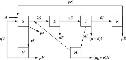
The chicken population at any time t, denoted by N(t) is divided into five subpopulations based on the disease status as follows; susceptible chickens who are at risk of acquiring coccidiosis disease, S(t), vaccinated chicken, V(t), chicken infected with a coccidiosis disease who are capable of transmitting the infection to susceptible chicken, I(t), and the recovered chicken, R(t). The number of coccidiosis viruses in a contaminated environment is denoted by H(t). It is assumed that chickens are recruited at a constant rate Λ. Susceptible chickens are vaccinated at rate τ in which vaccinated chickens who did not respond to vaccination wane out at the rate η and become susceptible again. It is also assumed that a susceptible chicken can be infected with coccidiosis if it comes into effective contact with an infectious chicken at a force of infection λ = βI + αH, where β denotes transmission rate for infectious chicken and α denotes ingestion rate of coccidiosis pathogen by chicken. Infected chicken shed pathogens into the environment at a rate ϵ. The term pathogens refers to infectious agents that course infection and illness in the chickens. These pathogens are shed from an infected chicken through its feces, containing oocysts. These oocysts can spread and contaminate the environment including water, food, and litter [14]. A newly infected chicken can progress to the infectious chicken class at rate γ. Sanitation is very important as it leads to the death of the coccidiosis pathogen. By so doing, the number of infections may significantly be reduced. Furthermore, it is assumed that the infected chicken in the I(t) compartment receives treatment at a rate θ. Moreover, all recovered chickens acquire temporary immunity, which wanes out at the rate ψ and becomes susceptible again. The disease-induced mortality occurs in the compartment, I(t) at rate δ. The pathogens deplete naturally at a rate μ_h or by sanitation measures at the rate ρ. All chickens in different subgroups experience natural death at a rate μ. The model flow diagram is in Figure 1.

Details are in the caption following the image — **Figure 1**
Open in figure viewer PowerPoint

The schematic diagram for the transmission dynamics of coccidiosis in chicken population.

Putting together all assumptions and model descriptions, we obtain the following system of nonlinear differential equations:

()

where λ = βI + αH.

The initial conditions of the model system (1) are S(0) ≥ 0, V(0) ≥ 0, E(0) ≥ 0, I(0) ≥ 0, R(0) ≥ 0, and H(0) ≥ 0.

3. Model Analysis

3.1. Invariant Region

Since the model system (1) deals with human beings, it is assumed that all parameters and variables in the model are nonnegative for all t ≥ 0. The discussion on the invariant region involves the description of the region in which the solution of the system makes epidemiological sense. We state and prove the following theorem.

Theorem 1. The region is positively invariant under the flow induced by the model system (1).

Proof. Consider the population size: N(t) = S(t) + V(t) + E(t) + I(t) + R(t) + H(t) and the rate of change given by:

()

From Equation (2) we have:

()

Solving Equation (3) for N yields implying that as t → ∞, where c is the constant of integration. Therefore, the feasible region solution set of the system enters the region Ω. Thus, the region Ω is a positively invariant set under the flow induced by the model and the model is well-posed and also it is biologically meaningful.

3.2. Positivity of the Solutions

In this section, we describe the positivity of the solution of the model system.

Theorem 2. The solution set (S(0), V(0), E(0), I(0), R(0)H(0)) > 0} of the model system (1) is positive for all t ≥ 0.

Proof. Consider the first equation of the model system (1):

()

It follows that

()

Integrating Equation (5) by separation of variables, we obtain:

()

where K is the constant of integration.

Applying the initial conditions S(0), in Equation (6) gives:

()

Similarly, the remaining other equations in the model system (1) give the following results:

()

Therefore, the solutions of the model are positive for all values of t > 0.

3.3. Existence of Equilibrium

In this part, we shall establish the equilibrium point. To find the existence equilibrium of the model, the right-hand side of the model system (1) is equated to zero. Thus, we have the following model system:

()

given that

()

The equilibrium of the model system is therefore given by E_∗ = S^∗, V^∗, E^∗, I^∗, R^∗, H^∗ as follows:

()

where

()

Then, substituting E^∗ into I^∗ from Equation (11), we obtain:

()

where

()

Now, solving Equation (13), we obtain one of the solution is I^∗ = 0, which represent the existence of disease-free equilibrium (DFE) and the remaining equation as follows:

()

indicate the existence of the endemic equilibrium point.

3.4. Disease-Free Equilibrium (DFE) Point

DFE is obtained in the absence of infection: It always exists when I = 0. Substitute I = 0 into equations in model system (9) to get:

()

Therefore, the DFE is given by:

()

3.5. The Effective Reproduction Number

The reproduction number that is used to investigate whether an infection introduced into a population will be eliminated or become endemic is obtained. It is defined as the expected number of secondary cases produced in a completely susceptible population by a typical infectious individual during its period of infectiousness [15, 16].

Following the ideas in [15, 17–19], the effective reproduction number R_e, is obtained by using the next-generation matrix method, which is given by the next-generation matrix’s spectral radius. We can rewrite the equations in the model system (1) starting with infectious classes first and then the rest follow. This leads to the following system:

()

From system (18) F_i and V_i are obtained as follows:

()

where λ = βI + αH and

()

The partial differentiation of F_i and V_i with respect to E, I, and H gives:

()

At DFE point (by substituting E⁰), we get:

()

Thus, FV⁻¹ is computed and given as follows:

()

Therefore, the eigenvalues of matrix FV⁻¹ are λ₁ = 0, λ₂ = 0, and λ₃ = (βa₆ + αϵ)γS⁰/a₃a₄a₆. Thus, the effective reproduction number is as follows:

()

where S⁰ = Λa₂/a₁a₂ − ητ.

3.6. Endemic Equilibrium Point

The endemic equilibrium point is obtained when coccidiosis exists in the population. In this case, the endemic equilibrium point is obtained by solving Equation (15) and get:

()

Then, substituting Equation (28) to Equation (11) the endemic equilibrium E_∗ = (S^∗, V^∗, E^∗, I^∗, R^∗, H^∗), is explicitly given as follows:

()

Therefore, it can be noted that the model system (1) has a unique endemic equilibrium point when R_e > 1.

3.7. Local Stability of the DFE

Here, we investigate the local stability of the DFE of the model system (1). For local stability, the spread of infection depends on the initial size of the subpopulation. To prove the local stability of the DFE, the eigenvalues of the Jacobian matrix of the system computed at the DFE point are obtained. The Jacobian matrix is obtained from the linearization of the model system (1). The Jacobian matrix J evaluated at DFE point, (E₀) is given by:

()

where a₁, a₂, a₃, a₄, a₅, and a₆ have the same meaning as in Equation (12) The DFE point is stable if all eigenvalues of the Jacobian matrix at the DFE point are negative. The eigenvalues of the Jacobian matrix (27) are established from the characteristic equation |J − λI| = 0. To obtain the eigenvalues of Equation (27):

()

The model system (28) can be written as follows:

()

It follows that:

()

From system (30), we have negative eigenvalue:

()

the polynomial equation

()

and matrix

()

Simplify the polynomial Equation (32) to obtain:

()

By Routh–Hurwitz criteria [16] the polynomial Equation (34) have negative root if a₁a₂ > τη. Furthermore, the two eigenvalues λ₂ and λ₃ in Equation (34) can be rewritten as follows:

()

The rest of the eigenvalues are the roots of the polynomial obtained in Jacobian matrix (33) which is given by:

()

where

()

By Routh–Hurwitz criteria the third-order polynomial Equation (36) has all roots in the open left half-plane if C₀, C₁, C₂ are positive and C₁C₂ > C₀ [16]. It is clear that C₂ is positive, and C₁ is positive if a₆(a₃ + a₄) + a₃a₄ > βγS⁰. Thus, we need to see the condition for C₀ > 0.

()

From Equation (38), C₀ is positive if R_e < 1. Hence, we have the following result.

Theorem 3. The DFE point is locally asymptotically stable if R_e < 1 and unstable if the inequality is reversed.

3.8. Global Stability of DFE

For global stability, the spread of the infection is independent of the initial size of the population. By using the comparison method [20], we establish the following theorem.

Theorem 4. The DFE is globally asymptotically stable if R_e < 1 and unstable if the inequality is reversed.

Proof. Let F and V be the Jacobian matrices of F_i and V_i defined as and ; 1 ≤ i, j ≤ m, where x is the number of individuals in each compartment, x₀ is a DFE, F_i is the rate of appearance of new infections in compartment i, , in which is the transfer rate of individuals into compartment i and is the rate of transfer of individuals out of compartment i. The rate of change of variables representing the infected components of the model system (1) can be rewritten as follows:

()

implying that

()

where the matrices F and V are defined as follows:

()

where a₃, a₄, a₆, and S⁰ have the same meaning as it is in Equations (12) and (37), respectively.

The matrix (F − V) is given by:

()

The eigenvalues of matrix (43) are established from the characteristic equation |J₂(G) − λI| = 0.

()

The polynomial obtained in matrix (44) is given by:

()

where

()

By Routh–Hurwitz criteria, the third-order polynomial Equation (45) has all roots in the open left half-plane if D₀, D₁, D₂ are positive and D₁D₂ > D₀ [16]. It is clear that D₂ is positive, and D₁ is positive if a₆(a₃ + a₄) + a₃a₄ > βγS⁰. Also, from Equation (46) D₀ is positive if R_e < 1. This result signifies that the eigenvalues of matrix (F − V) have negative real parts if R_e < 1. Therefore, system (1) is stable for R_e < 1. It follows that (E⁰, I⁰, H⁰) → (0, 0, 0) as t → ∞. Furthermore, examining the first, second, third, fourth, fifth, and sixth equations of system (9), gives S = Λa₂/a₁a₂ − ητ, and V = τΛ/a₁a₂ − ητ whenever E⁰ = I⁰ = H⁰ = 0. Therefore, by employing the comparison method [21] it follows that (S⁰, V⁰, E⁰, I⁰, R⁰) → (Λa₂/a₁a₂ − ητ, τΛ/a₁a₂ − ητ, 0, 0, 0, 0) as t → ∞ for R_e < 1. Hence, E₀ is globally asymptotically stable whenever R_e < 1. Thus, the system will come to a DFE point from any starting point.

3.8.1. The Impact of Intervention Strategies

The effects of implementing intervention strategies are investigated. Since, the interventions have been invested in controlling pneumonia disease, it is very important to understand the benefits of implementing these interventions. The three intervention strategies’ contribution is observed by comparing the basic reproduction number and the effective reproduction number.

Consider the reproduction number in the presence of all three interventions as presented in Equation (47):

()

where

()

Substituting Equation (48) in Equation (47) gives:

()

The basic reproduction number (the reproduction number of the model in the absence of interventions) is given by:

()

Then, the reproduction number (R_e) in the presence of all three interventions can be presented as follows:

()

where

()

In Equation (52),

()

This indicates that the value of the numerator is less than the value of the denominator. Consequently, it implies that k < 1. This demonstrates that vaccination, treatment, and sanitation effectively curb initial disease transmission and halt-epidemic spread.

3.9. Bifurcation Analysis

The presence of forward or backward bifurcations has a significant impact on infectious disease epidemiological control efforts. The bifurcation analysis of the equilibrium points determines whether the disease can be entirely eradicated or whether it will remain in the population. The bifurcation analysis is carried out at the DFE using the center manifold theory proposed by Castillo-Chavez and Song [22]. This is accomplished by renaming the model’s state variables of the model system (1) as follows: let x₁ = S, x₂ = V, x₃ = E, x₄ = I, X₅ = R, and x₆ = H and the system can be written in the form of:

()

where X_i =

, F =

, and (.)^T denote a matrix transpose. The model system (1) takes the form:

()

Let β^∗ be the bifurcation parameter, then, system (55) is linearized at a DFE point when β = β^∗ with R_e = 1. Hence, solving for β^∗ from R_e = 1 in Equation (47) gives:

()

Then, the linearized system (55) is transformed with β = β^∗ which has a simple zero eigenvalue, and center manifold theory is used to analyze the dynamics of Equation (55) near β = β^∗. Thus, the Jacobian matrix of system (55) at DFE E₀ denoted by J(β^∗) is given by:

()

where k₁ = Λa₂/a₁a₂ − ητ.

Then, the right and left eigenvectors corresponding with the zero eigenvalues are now computed. ω = [ω₁, ω₂, ω₃, ω₄, ω₅, ω₆]T gives the right eigenvector associated with the zero eigenvalue, and the following equations are obtained:

()

Solving system (58) for

, i = 1, 2, …, 6, gives the following right eigenvectors:

()

Furthermore, to calculate the left eigenvectors given by

which satisfy v.ω = 1, the matrix J(β^∗) should be transposed and becomes:

()

Then, solving

, the following equations are obtained:

()

Solving system (61) for

, i = 1, 2, …, 9, the following left eigenvectors are obtained:

()

To establish the conditions for the occurrence of forward or backward bifurcations, the Castillo-Chavez and Song Theorem 4.1 in [22] is used. The theorem is provided below for easy reference since it is important for providing the local stability of the endemic equilibrium point around R₀ = 1.

Theorem 5. Consider the following general system of ordinary differential equations with a parameter ϕ such that

()

where 0 is an equilibrium point of the system (that is, f(0, ϕ)≡0 for all ϕ) and

(1)
is the linearization matrix of system (63) around the equilibrium 0 with ϕ evaluated at 0.
(2)
Zero is a simple eigenvalue of A, and all other eigenvalues of A have negative real parts.
(3)
Matrix A has a nonnegative right eigenvector ω and a left eigenvector v corresponding to the zero eigenvalue.

Let f_k be the k^th components of f and

()

The local dynamics of the system around the equilibrium point are totally determined by the signs of a and b for |ϕ| < 1,

(i)
a > 0, b > 0. When ϕ < 0, 0 is locally asymptotically stable and there exists a positive unstable equilibrium; when 0 < ϕ < 1, 0 is unstable and there exists a negative, locally asymptotically stable equilibrium.
(ii)
a < 0, b < 0. When ϕ < 0, 0 is unstable; when 0 < ϕ < 1, 0 is asymptotically stable equilibrium, and there exists a positive unstable equilibrium.
(iii)
a > 0, b < 0. When ϕ < 0, 0 is unstable, and a positive unstable equilibrium appears.
(iv)
a < 0, b > 0. When ϕ changes from positive to negative, 0 changes its stability from stable to unstable. Correspondingly, a negative unstable equilibrium becomes positive and locally asymptotically stable.

Particularly, if a > 0, and b > 0, then, a subcritical (or backward) bifurcation occurs at ϕ = 0.

To govern the local dynamics of the transformed system (55), the values of a and b are determined to explore whether the model system (55) exhibits forward or backward bifurcation. For system (55), the associated nonzero second-order partial derivatives at DFE and β = β^∗ are given by:

()

Therefore,

()

a > 0 if v₁ < 0 and a < 0 if v₁ > 0 as a is positive if (ω₁ω₄β + ω₁ω₆α)v₃ > (ω₁ω₄β + ω₁ω₆α)v₁ and a is negative if (ω₁ω₄β + ω₁ω₆α)v₃ < (ω₁ω₄β + ω₁ω₆α)v₁.

For the sign of b, it can be shown that the associated nonvanishing partial derivatives are as follows:

()

Then, it follows from the above expression that:

()

b > 0 if v₁ < 0 and a₁a₂ > ητ otherwise b will be <0.

Theorem 6. The unique endemic equilibrium is ensured, and by Theorem 5, the model is locally asymptotically stable for R₀ > 1. Moreover, according to Theorem 5 item (i), the model experiences backward bifurcation when a > 0. This is true only if v₁ < 0, and a₁a₂ < ητ are present; otherwise, forward bifurcation occurs.

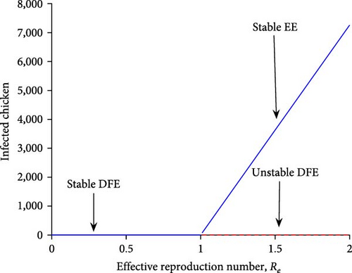
The model system (1) exhibits forward bifurcation at R₀ = 1 when a < 0 and b > 0. Biologically, this scenario demonstrated that the model system (1) is globally asymptotically stable at a DFE point when R₀ < 1, and has a distinct endemic equilibrium point for R₀ > 1. When R₀ is close to one the unique endemic equilibrium point is locally asymptotically stable. When R₀ falls below one, that is R₀ < 1 no endemicity exists and the disease continues to decline, and as R₀ increases to above one, that is R₀ > 1, the disease invades the population. Furthermore, when a > 0 and b > 0, the model system (1) exhibits a backward bifurcation, as R₀ approaches one, the disease prevalence rapidly increases giving rise to a situation in which the DFE co-exists with the endemic equilibrium. The biological implication of backward bifurcation is that the classical requirements of having the reproduction number less than unity, although necessary, is no longer sufficient for disease eradication. Based on Equation (15), The model system (1) exhibit a forward bifurcation as shown in Figure 2.

Table 1. Values of sensitivity indices.

Parameters	Sensitivity index for R_e < 1	Sensitivity index for R₀ > 1
Λ	+ 1	+1
β	+0.0805	+ 0.7820
α	+0.2180	+0.9195
μ	−0.04383	−0.0944
γ	+0.3733	+0.3733
θ	−0.1068	—
δ	−0.2137	−0.2392
η	+0.0042	—
τ	−0.0118	—
ϵ	+0.1111	+0.7999
ρ	−0.2127	—
μ_h	−0.0053	−0.9195

Table 2. Parameters and their descriptions for the coccidiosis dynamic model Equation (1).

Parameter	Descriptions	Values	Source
Λ_h	Chicken recruitment rate	0.001/day	Assumed
β	Transmission rate for infectious chicken	0.7/day	Assumed
α	Eimeria transmission rate due to the chicken-to-environment interaction	0.8/day	Assumed
μ	Nature death rate of a chicken	1.37 − 5.48 × 10⁻⁴/day	[27]
γ	Chicken incubation rate	0.09/day	Assumed
θ	Chicken recover rate/treatment rate	0.01/day	Assumed
ψ	Immunity waning rate for the recovered chicken	0.09/day	Assumed
δ	Chicken death rate due to coccidiosis	0.02/day	Assumed
η	Waning rate of vaccinated chicken	0.03/day	Assumed
τ	Rate at which susceptible chicken are vaccinated	0.001/day	Assumed
μ_h	Parasite natural death rate	0.001/day	[13]
ρ	Eimeria death rate due to sanitation measures	0.04/day	Assumed
ϵ	Parasite shedding rate to the environment by infectious chicken	0.4/day	[13]

3.10. Global Stability of the Endemic Equilibrium Point

This section applies the Korobeinikov technique, as employed in the work of [23], to examine the global stability of the endemic equilibrium point E_∗. Using this method, an appropriate Lyapunov function is created in the form of:

()

where A_i is a nonnegative constant, x_i is the population of the i^th subpopulation, and

is the endemic equilibrium point E_∗. Therefore, the following Lyapunov function is developed as follows:

()

Given that A₁, A₂, A₃ … A₆ are nonnegative constants whereby V is Lyapunov function. The selection of the function V and its constant ensures that it is continuous and differentiable in space at all times. Differentiating V with respect to time gives:

()

The following is therefore obtained by substituting equations of the model system (1)–(71).

()

The following are obtained at the endemic equilibrium point:

()

Then, by substituting Equation (73) to Equation (72) and doing some simplifications, we obtain:

()

given that

()

Then, if S = S^∗, V = V^∗, E = E^∗, I = I^∗, R = R^∗, H = H^∗, the function (75) becomes less than or equal to zero and for all S, V, E, I, R, H > 0, following the approach of Korobeinikov [23]. Hence, the largest compact invariant set in {S, V, E, I, R, H} where is the singleton {S^∗, V^∗, E^∗, I^∗, R^∗, H^∗} which is the endemic equilibrium point of the model system (1). It is implied that {S^∗, V^∗, E^∗, I^∗, R^∗, H^∗} is globally asymptotically stable in the interior region of {, V, E, I, R, H} by Lasalle’s invariant principle [24]. As a result, the following theorem is provided:

Theorem 7. If R₀ > 1, then the coccidiosis model (1) has a unique endemic equilibrium point S^∗, V^∗, E^∗, I^∗, R^∗, H^∗ which is globally asymptotically stable in S, V, E, I, R, H.

3.11. Sensitivity Analysis

Sensitivity indices measure the relative change in a state variable when a parameter change [25]. Initial disease transmission is directly related to the reproduction number. The sensitivity analysis is performed to determine which model parameters are the most important to disease transmission and prevalence (the parameters that are the most sensitive with respect to the initial transmission of the disease). In this study, we use it to discover parameters that have a high impact on reproduction number, and should be targeted by intervention strategies [26]. If a variable is a differentiable function of the parameter, the sensitivity indices may be alternatively defined using partial derivatives [25]. We intend to know how each parameter affects the effective reproduction number R_e. We use the formula of the normalized sensitivity index of a variable for R_e to achieve our goal.

The normalized forward sensitivity index of a variable, Z, depends differentiability on index of a parameter, ϕ is defined as follows:

()

Applying the formula for R₀ and R_e, we have:

()

Applying the normalized forward sensitivity index defined in Equations (77) and (78) yields to the results in Table 1. The parameter values in Table 2 are used to determine the sensitivity indices.

3.11.1. Interpretation of Sensitivity Indices

The sensitivity indices are presented in Table 1, when R₀ > 1 (in the absence of intervention) and when R_e < 1 (in the presence of interventions). Parameters that have positive sensitivity indices in Table 1, indicated that if their values are increased while keeping other values constant, reproduction number increases. These parameters have a greater influence on spreading the coccidiosis infection. But the parameters with negative sensitivity indices, show that if their values are increased while keeping the rest parameters fixed, reproduction number decreases. The most sensitive parameter is Λ with positive sensitivity indices. Other parameters with greater positive sensitivity indices are β, α, and γ. These parameters have an impact on reproduction number, and should be targeted for intervention strategies. These findings can be used to inform the development of intervention strategies to control coccidiosis infection. For example, interventions that target reducing the rate of transmission, such as vaccination or improved hygiene, are likely to be most effective.

3.12. Numerical Analysis

In this section, the model system (1) was numerically solved using MATLAB software and the Runge–Kutta fourth-order approach. To support previously analytical findings, various graphical representations are provided and discussed. Since many parameters were not publicly available, we collected a few from the literature and others were assumed for demonstration. For simulation, the study employed the initial values of the parameters from Table 2. The following initial values for the subpopulation were assumed as follows: S(0) = 400, V = 300, E = 100, I = 100, R = 80, and H = 5, 000.

3.13. Effects of Interventions on Infected Chickens

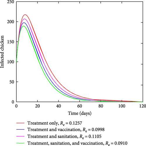
Figure 3 depicts how the number of exposed and infected chickens changes over time. It can be observed from Figures 3(a) and 3(b) that the number of exposed and infected chickens decreases as time increases when there are interventions and increases when there are no interventions. This finding implies that the prevention measures of treatment, vaccination, and sanitation have a positive impact on reducing the spread of coccidiosis in the population.

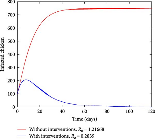
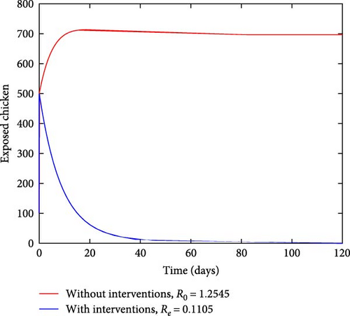
Figure 4 depicts how the number of exposed and infected chickens changes over time. It can be observed from Figures 4(a) and 4(b) that the number of exposed and infected chickens decreases as time increases when there are interventions and increases when there are no interventions. This finding implies that the prevention measures of treatment, vaccination, and sanitation have a positive impact on reducing the spread of coccidiosis in the population.

3.14. Effect of Varying Some Parameter Values

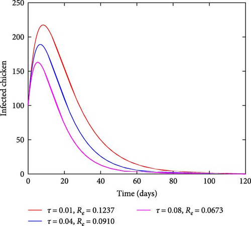
Figure 5 illustrates the effects of varying treatment rates. As the rate of treating the infected chicken increases, the number of infected chickens also reduces, as shown in Figure 5(a). On the other hand, by increasing the treatment rates, the number of recovered chickens increases with time as shown in Figure 5(b). This result indicates that treating the affected chicken has a significant effect on curbing coccidiosis as it reduces the number of sick chickens and increases the number of recovered individuals in the population.

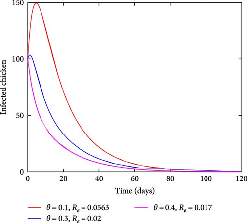
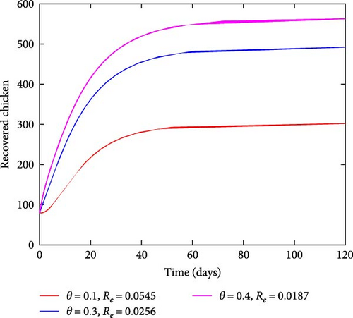
Figure 6 shows the impact of sanitation on infected chickens and Eimeria pathogen population. The findings show that when sanitation rates increase, the number of both infected chickens and pathogens decreases as time passes as shown in Figures 6(a) and 6(b). This finding demonstrated that cleanliness has a major role in the complete eradication of coccidiosis disease in the population.

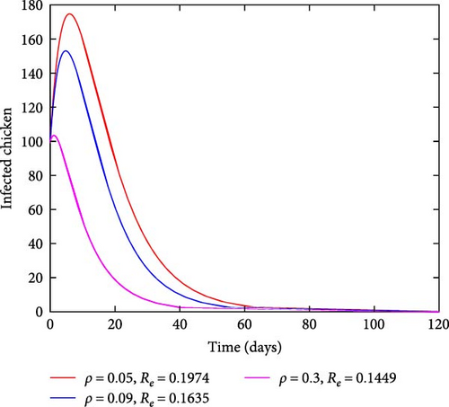
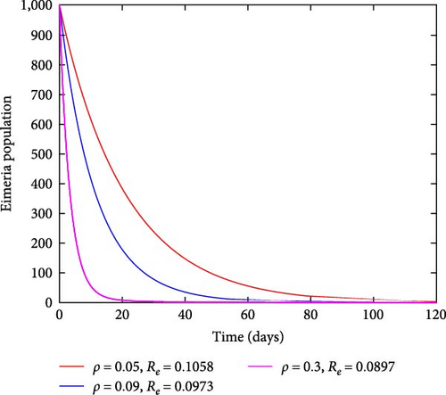
In this instance, the focus was to evaluate the contribution made by the sanitation strategy toward eradicating the coccidiosis epidemic in the community. Figure 7 findings demonstrate that when sanitation rates increase, the number of infected chickens significantly decreases. In this strategy, efforts like adequate waste disposal and hygienic practice follow-up may be practiced with the main objective of limiting the spread of this disease in the community.

4. Conclusion

A deterministic model with control interventions for chicken coccidiosis disease is derived and analyzed to investigate the effect of each control intervention for controlling this disease. The effective reproduction number and equilibria of the model are derived. The stability analysis of the DFE is derived, and it is stable when the reproduction number is less than unity. Also, the contribution of the control interventions is assessed by comparing the basic reproduction number (R₀) and effective reproduction number (R_e), whereby it is observed that R_e < R₀. This result implies that the control interventions (vaccination, sanitation, and treatment) reduce the transmission rate of the disease. On the other hand, sensitivity analysis carried out on the model parameters shows that: the control parameters (θ (treatment), ρ (sanitation), and τ (vaccination)) are the essential parameters for effective control of the disease, as they have negative indices. Numerical analysis of the model system (1) is carried out to illustrate the effectiveness of the control interventions. The results show that as the rate of the control parameters increases, the number of infected chicken and coccidiosis pathogens decreases. The results further show that applying the control interventions singly or in combination reduces the infection rate, though the combination has the most significant results. The model discussed in this paper is not exhaustive. As a result, the model’s underlying assumptions can be adjusted to include the aspect of the age structure of the chicken, the role of seasonal variations on the transmission dynamics of coccidiosis in the chicken population, or optimal and cost-effectiveness.

Conflicts of Interest

The authors declare that they have no conflicts of interest.

Acknowledgments

Y. Liana would like to appreciate the support provided by the College of Business Education, Tanzania. M. Swai is grateful for the support provided by the Open University of Tanzania.

Open Research

Data Availability

All data and materials that support the findings of this research study are included in the paper.

References

1 Mesa-Pineda C., Navarro-Ruíz J. L., López-Osorio S., Chaparro-Gutiérrez J. J., and Gómez-Osorio L. M., Chicken coccidiosis: from the parasite lifecycle to control of the disease, Frontiers in Veterinary Science. (2021) 8, https://doi.org/10.3389/fvets.2021.787653, 787653.
10.3389/fvets.2021.787653
PubMed Web of Science® Google Scholar
2 McDougald L. R., Cervantes H. M., Jenkins M. C., Hess M., and Beckstead R., Protozoal infections, Diseases of Poultry. (2020) 1192–1254, https://doi.org/10.1002/9781119371199.
10.1002/9781119371199.ch28
Google Scholar
3 Nabian S., Arabkhazaeli F., Seifouri P., and Farahani A., Morphometric analysis of the intestine in experimental coccidiosis in broilers treated with anticoccidial drugs, Iranian Journal of Parasitology. (2018) 13, no. 3, 493–499.
PubMed Web of Science® Google Scholar
4 Morishita T. Y. and Greenacre C. B., Backyard Poultry Medicine and Surgery: A Guide for Veterinary Practitioners”, 2021, John Wiley & Sons.
Google Scholar
5 Hauck R., Carrisosa M., McCrea B. A., Dormitorio T., and Macklin K. S., Evaluation of next-generation amplicon sequencing to identify Eimeria spp. of chickens, Avian Diseases. (2019) 63, no. 4, 577–583, https://doi.org/10.1637/aviandiseases-D-19-00104.
10.1637/aviandiseases-D-19-00104
PubMed Web of Science® Google Scholar
6 Zou W., Yu H., Wang X., G. Dai M. Sun, Zhang G., Zhang T., Shi H., Xie K., and Wang J., Establishing a model for evaluating chicken coccidiosis resistance based on principal component analysis, Animals. (2019) 9, no. 11, https://doi.org/10.3390/ani9110926, 926.
10.3390/ani9110926
PubMed Web of Science® Google Scholar
7 Peek H. W. and Landman W. J. M., Coccidiosis in poultry: anticoccidial products, vaccines and other prevention strategies, Veterinary Quarterly. (2011) 31, no. 3, 143–161, https://doi.org/10.1080/01652176.2011.605247, 2-s2.0-83455179568.
10.1080/01652176.2011.605247
CAS PubMed Web of Science® Google Scholar
8 Peek H. W., Resistance to Anticoccidial Drugs: Alternative Strategies to Control Coccidiosis in Broilers”, 2010, Utrecht University.
Google Scholar
9 Khan A., Abdeljawad T., and Alqudah M. A., Neural networking study of worms in a wireless sensor model in the sense of fractal fractional, AIMS Mathematics. (2023) 8, no. 11, 26406–26424, https://doi.org/10.3934/math.20231348.
10.3934/math.20231348
Web of Science® Google Scholar
10 Bedi P., Khan A., Kumar A., and Abdeljawad T., Computational study of fractional-order vector borne diseases model, Fractals-an Interdisciplinary Journal on The Complex Geometry of Nature. (2022) 30, no. 5, https://doi.org/10.1142/S0218348X22401491, 2240149.
10.1142/S0218348X22401491
Google Scholar
11 Kachanova E. O., Chalysheva E. I., Andreyanov O. N., and Safiullin R. T., Experimental model of coccidiosis caused by Eimeria Tenella in broiler chickens, Journal of World’s Poultry Research. (2019) 9, no. 4, 262–267, https://doi.org/10.36380/scil.2019.wvj33.
10.36380/scil.2019.wvj33
Google Scholar
12 Johnston W. T., Shirley M. W., Smith A. L., and Gravenor M. B., Modelling host cell availability and the crowding effect in Eimeria infections, International Journal for Parasitology. (2001) 31, no. 10, 1070–1081, https://doi.org/10.1016/S0020-7519(01)00234-X, 2-s2.0-0034960591.
10.1016/S0020-7519(01)00234-X
CAS PubMed Web of Science® Google Scholar
13 Vermeulen A. N., Schaap D. C., and Schetters T. P. M., Control of coccidiosis in chickens by vaccination, Veterinary Parasitology. (2001) 100, no. 1-2, 13–20, https://doi.org/10.1016/S0304-4017(01)00479-4, 2-s2.0-0035850576.
10.1016/S0304-4017(01)00479-4
CAS PubMed Web of Science® Google Scholar
14 Gharekhani J., Sadeghi-Dehkordi Z., and Bahrami M., Prevalence of coccidiosis in broiler chicken farms in Western Iran, Journal of Veterinary Medicine. (2014) 2014, 4, https://doi.org/10.1155/2014/980604, 980604.
10.1155/2014/980604
PubMed Google Scholar
15 Diekmann O., Heesterbeek J. A., and Metz J. A., On the definition and the computation of the basic reproduction ratio R0 in models for infectious diseases in heterogeneous populations, Journal of Mathematical Biology. (1990) 28, no. 4, 365–382, https://doi.org/10.1007/BF00178324, 2-s2.0-0025159677.
10.1007/BF00178324
CAS PubMed Web of Science® Google Scholar
16 Martcheva M., An Introduction to Mathematical Epidemiology”, 2013, Springer, New York.
Google Scholar
17 van den Driessche P. and Watmough J., Reproduction numbers and sub-threshold endemic equilibria for compartmental models of disease transmission, Mathematical Biosciences. (2002) 180, no. 1-2, 29–48, https://doi.org/10.1016/S0025-5564(02)00108-6, 2-s2.0-0036845274.
10.1016/S0025-5564(02)00108-6
CAS PubMed Web of Science® Google Scholar
18 Liana Y. A., Shaban N., Mlay G., and Phibert A., African trypanosomiasis dynamics: modelling the effects of treatment, education, and vector trapping, International Journal of Mathematics and Mathematical Sciences. (2020) 2020, 15, https://doi.org/10.1155/2020/3690472, 3690472.
10.1155/2020/3690472
Google Scholar
19 Liana Y. A. and Chuma F. M., Mathematical modeling of giardiasis transmission dynamics with control strategies in the presence of carriers, Journal of Applied Mathematics. (2023) 2023, 14, https://doi.org/10.1155/2023/1562207, 1562207.
10.1155/2023/1562207
Google Scholar
20 Swai M. C., Shaban N., and Marijani T., Optimal control in two strain pneumonia transmission dynamics, Journal of Applied Mathematics. (2021) 2021, 21, https://doi.org/10.1155/2021/8835918, 8835918.
10.1155/2021/8835918
Google Scholar
21 Shaban N., Modelling the effects of public health education in the spread of hepatitis B disease, Applied Mathematical Sciences. (2015) 9, no. 80, 3967–3981, https://doi.org/10.12988/ams.2015.44289, 2-s2.0-84936853223.
10.12988/ams.2015.44289
Google Scholar
22 Castillo-Chavez C. and Song B., Dynamical models of tuberculosis and their applications, Mathematical Biosciences & Engineering. (2004) 1, no. 2, 361–404, https://doi.org/10.3934/mbe.2004.1.361.
10.3934/mbe.2004.1.361
PubMed Web of Science® Google Scholar
23 Korobeinikov A., Global properties of infectious disease models with nonlinear incidence, Bulletin of Mathematical Biology. (2007) 69, no. 6, 1871–1886, https://doi.org/10.1007/s11538-007-9196-y, 2-s2.0-34547655762.
10.1007/s11538-007-9196-y
PubMed Web of Science® Google Scholar
24 La Salle J. P., The stability of dynamical systems, CBMS-NSF Regional Conference Series in Applied Mathematics, 1976, SIAM, Philadelphia.
10.1137/1.9781611970432
Google Scholar
25 Chitnis N., Hyman J. M., and Cushing J. M., Determining important parameters in the spread of malaria through the sensitivity analysis of a mathematical model, Bulletin of Mathematical Biology. (2008) 70, no. 5, 1272–1296, https://doi.org/10.1007/s11538-008-9299-0, 2-s2.0-47349102730.
10.1007/s11538-008-9299-0
PubMed Web of Science® Google Scholar
26 Prieto K. and Ibarguen-Mondragon E., Parameter estimation, sensitivity and control strategies analysis in the spread of influenza in Mexico, Journal of Physics: Conference Series. (2019) 1408, no. 1, https://doi.org/10.1088/1742-6596/1408/1/012020, 012020.
10.1088/1742-6596/1408/1/012020
Google Scholar
27 Sanchez J., Lama J. R., Peinado J., Paredes A., Lucchetti A., Russell K., Kochel T., and Sebastian J. L., High HIV and ulcerative sexually transmitted infection incidence estimates among men who have sex with men in Peru: awaiting for an effective preventive intervention, JAIDS Journal of Acquired Immune Deficiency Syndromes. (2009) 51, no. Supplement 1, S47–S51, https://doi.org/10.1097/QAI.0b013e3181a2671d, 2-s2.0-66149131094.
10.1097/QAI.0b013e3181a2671d
PubMed Web of Science® Google Scholar

Citing Literature

All articles

Mathematical Modeling of Coccidiosis Dynamics in Chickens with Some Control Strategies

Abstract

1. Introduction

2. Model Description and Formulation

3. Model Analysis

3.1. Invariant Region

3.2. Positivity of the Solutions

3.3. Existence of Equilibrium

3.4. Disease-Free Equilibrium (DFE) Point

3.5. The Effective Reproduction Number

3.6. Endemic Equilibrium Point

3.7. Local Stability of the DFE

3.8. Global Stability of DFE

3.8.1. The Impact of Intervention Strategies

3.9. Bifurcation Analysis

3.10. Global Stability of the Endemic Equilibrium Point

3.11. Sensitivity Analysis

3.11.1. Interpretation of Sensitivity Indices

3.12. Numerical Analysis

3.13. Effects of Interventions on Infected Chickens

3.14. Effect of Varying Some Parameter Values

4. Conclusion

Conflicts of Interest

Acknowledgments

Open Research

Data Availability

References

Citing Literature

Figures

References

Information

About Wiley Online Library

Help & Support

Opportunities

Connect with Wiley

Mathematical Modeling of Coccidiosis Dynamics in Chickens with Some Control Strategies

Abstract

1. Introduction

2. Model Description and Formulation

3. Model Analysis

3.1. Invariant Region

3.2. Positivity of the Solutions

3.3. Existence of Equilibrium

3.4. Disease-Free Equilibrium (DFE) Point

3.5. The Effective Reproduction Number

3.6. Endemic Equilibrium Point

3.7. Local Stability of the DFE

3.8. Global Stability of DFE

3.8.1. The Impact of Intervention Strategies

3.9. Bifurcation Analysis

3.10. Global Stability of the Endemic Equilibrium Point

3.11. Sensitivity Analysis

3.11.1. Interpretation of Sensitivity Indices

3.12. Numerical Analysis

3.13. Effects of Interventions on Infected Chickens

3.14. Effect of Varying Some Parameter Values

4. Conclusion

Conflicts of Interest

Acknowledgments

Open Research

Data Availability

References

Citing Literature

Figures

References

Related

Information