1. Introduction

Quantum machine learning (QML) is a subconcept of quantum computational data and information processing research in which the main target is developing the QML algorithms that can learn from data to improve the existing classical learning methods in machine learning [1]. Here, quantum computers can process data in the form of qubits rather than bits and this computer can have also its own architecture. For this architecture, it is impossible to apply classical machine learning methods directly to learn and process the data. A quantum machine learning algorithm can be implemented on a quantum computer; this computer can exploit the laws of the quantum mechanical model (quantum theory) to process the data and to predict the outcome. Aimed to investigate the applicability of quantum computing advantage to solve such problems, the researcher proposed this study and developed quantum circuits for DRL to analyze the performance of quantum agents with different learning rates and different quantum layers. This study used the advantage of PennyLane provided by Xanadu to create circuits and the open gym benchmark-like frozen lake problem was solved. The expected optimization of the best policy action selection of a quantized agent to get maximum reward is analyzed and then the learning performance is stated. This can be achieved by calculating the quantum expectation value or expected energy value.

The main basis of quantum machine learning is to use the essential benefits of quantum computing technology such as quantum entanglement, quantum superposition, and quantum parallelism to increase the performance of classical machine learning algorithms [2–5]. Although they utilized the quantum mechanics’ concept of quantum entanglement and supper position, most of the quantum machine learning algorithms (QMLA) are borrowed from the basic concept and architecture of classical machine learning algorithms [6]. In other cases, some researchers used the hybrid classical-quantum architecture and proved that the use of classical-quantum hybrid systems can overcome the limitation of noise intermediate scale quantum (NISQ) computers [7, 8]. For example, Dunjko et al. [9] proposed the quantum approximate algorithm in which classical solution parameters to a problem can be used as an input and as the starting point for larger problems such as variational quantum eigen solvers. Recently, the experiment held by Parades et al. [10] proved that quantum machine learning has shown interesting results for machine learning applications where classical machine learning techniques are limited to perform because of inadequate training data and high dimensionality of the features. They proposed a PennyLane simulator-based hybrid classical-quantum model for transfer learning to enhance the classification of face images with a COVID-19 mask and resulted in an accuracy of 99.05% in classifying the exact protective masks. Lloyd et al. [11] also proposed quantum-inspiredk-means and nearest centroid algorithms through quantum distance approximation as we do have quantum access to the classical data. In quantum enhanced clustering algorithm, the execution time for a certain state of N vectors in feature space with dimension D of each iteration (by a distance approximation technique with error ε) is given by O(kN logD/ε). Generally, several works depict the incredible performance of the quantum-enhanced machine learning model for the problem with large feature spaces, which can be difficult for the classical machine learning algorithm to perform.

2. Related Works

By its nature, whether it is enhanced or not, deep reinforcement learning (DRL) is a machine learning in which the interaction takes place between an agent and the environment. In various real-worlddecision-making situations, there is no data on the best course of action. For such a scenario, the model must interfere with its surroundings in order to gather information and learn how to complete a task via its own experience. This learning method is called reinforcement learning (RL). For example, a video game character might learn a fruitful strategy by repetitively playing the game, examining the outcomes, and improving the future ways. In current studies of quantum enhanced RL [12, 13], variational quantum circuits (VQC) replace the policy of training the deep neural network (DNN) of existing deep reinforcement learning (DRL). At each experience in each episode, a quantum agent with particular state information decides its action from the policy of variational quantum circuits, and the classical optimizer such as RMsprop, Adam optimizer, and others are used to update the parameters. The action selection is based on the expected value of quantum measurement.

Though quantum deep reinforcement learning (QDRL) with designated parameterized quantum circuits (PQC) is a quite new field of study, some researchers such as Lockwood and Si [12] studied different encoding methods such as directional encoding and scaled-up encoding techniques and also pooled the parameterized circuit with quantum pooling operations to solve some reinforcement learning problems. This encoding technique is cost-efficient but requires a large number of quantum gates which are beyond the capabilities of actual quantum simulators.

The method used by Hu and Hu [14] uses common gates, but they investigated with less number of qubits. It needs some investigation to know what if the number of qubits increased. Here, the intention is to advance the intelligence of quantum agents, which can react with the environment and learn from it to reach some stated goal. In this sense, numerous works have provided suggestions in the last few years [9, 15–18]. Few of these deal with enhancing reward by quantizing an agent which interacts with a classical environment through Grover search. The others prove quantum speed up when both agents and environments had been quantized with quantum phenomena.

Table 1 shows the bird’s eye view of quantum, quantum-classical, and classical deep reinforcement learning. The learning algorithm can be enhanced either by quantizing an agent or an environment, or both. Quantum computers may be available only in large companies such as IBM, D-Wave, and Google for research purposes [9, 19]. For the reason of unavailability of such resources, we find a way for developing the hybrid and running the learning algorithms on current classical computers such as the method used by [15, 20, 21].

For the scenario of “quantum agent classical environment,” Dunjko et al. [9] suggested the Grovers iteration-based searching algorithm for unstructured search and investigates a potential quantum computing benefit when a quantized agent interacts with a classical environment and the study improves the quantum speedup over the classical computations. The other scenario of quantum-enhanced deep reinforcement learning comes with a “quantum agent quantum environment.” The proposed study by Lamata [22] and Albarran et al. [23] works on this scenario by considering the quantum agent and quantum environment interactions to investigate the possibility of implementations by increasing the extent of system complexity. Another prospect would be to investigate classical agent and quantum environment interactions which are made by applying the “classical agent-quantum environment” scenario. The study proposed by Daoyi Dong et al. [24] investigates the way of mapping conventional reinforcement learning into quantum reinforcement learning, and the study focuses on linking the previous states with future quantum states. According to the study with different learning parameters, there is a quadratic quantum speedup compared to the classical temporal difference (TD) by applying superposition and quantum entanglement on the quantum algorithms.

Some other researchers [9, 15–18] study the applicability of quantum computing on classical reinforcement learning. According to the study, variational quantum circuits can replace the policy training of deep neural networks in existing classical DRL. The interaction between the environment and an agent takes place based on the policy of quantum circuits. For each and every episode, an agent decides its action from the policy of quantum circuits, and the classical optimizer such as Adam optimizer is used to update the parameter [19]. This paper uses the same scenarios with different circuit designs and different environments.

3. Methods

3.2. Froze Lake Environment

For this paper, we have selected frozen lake (FL) grid environment for its simplicity in discrete state space. It comprises of a 4 × 4 grid demonstrating a frozen surface, where the agent can select to move one step down, up, right, or left. The aim is to cross the lake from the starting point of the top left corner to the endpoint of the bottom right corner. Nevertheless, the particular grid point of the environment corresponds to holes in the ice, and when the agent steps on them, the iteration of the episode terminates and it has to restart from the initial state. One of the following conditions makes the terminations of iterative episode:

• (1)

  The agent reaches the goal G

• (2)

  The agent iterates and reaches a maximum of 3000-time steps

• (3)

  The agent falls into a hole (red subgrid).

For each episode in which the goal is reached, the agent takes a reward of +1 for successfully reaching the goal, and −0.1 if the agent is stepping into one hole.

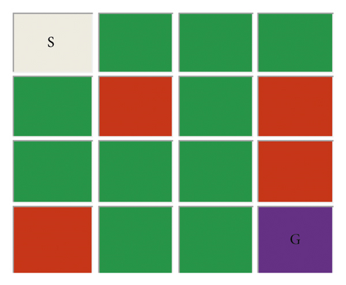
As shown in Figure 1 in frozen lake environment (extended from Hu and Hu [14]), it is expected from the quantum agent to move from the grid start location (S) found at the left-up corner to the right bottom corner goal location (G). The lake may not all be frozen which means there may be various holes (red color) on the path. It is the responsibility of the quantum agent to train and avoid walking into these hole locations, and if not, the quantum agent will get a huge negative reward, and then an episode iteration will be ended. To realize this, we have assigned a little negative return value to each wrong move. The frozen lake environment shown in Figure 1 has 16 eigen states (4 holes+ 12 frozen states) and 4 eigen actions (MoveTop, MoveDown, MoveLeft, and MoveRight). Without applying trainable input data weights, we encode each point on the grid as one of the computational basis states of a 4-qubit quantum system (|0000〉 … |1111〉).

From Table 2 , we have seen that most research studies have been performed in quantum reinforcement learning and they have realized the possibility of enhancing classical reinforcement learning with quantum computing. The literature depicts that the performance of the enhanced model was better than the classical one. Additionally, in the last five years, the study on the field of quantum computing has become significant and has grown as of frightening data increment and the idea of promising quantum computing technologies will change today’s computing world. This field got attention from various researchers of companies such as Google [34], IBM [35], and Microsoft [36], and they are racing to develop quantum computers and have realized the applicability of quantum computing technology in classical machine learning algorithms [37].

Table 2. Some quantum-enhanced ML algorithms we found from the literary review.

Related works of literature	OpenAI gym environment		Performance	Algorithm used by the researcher
Yueh Hsiao et al. [30]		Acrobot and LunarLander	Converged faster	Proximal policy optimization (PPO)
Lockwood and Si [31]		CartPole-v1 and Acrobot	Not defined	Policy gradient with baseline’
Lan [32]		Pendulum	Faster convergency	Soft actor-critic
Yun et al. [33]		CartPole-v0	Not defined	Q-Learning
Hu and Hu [14]		2 × 3 frozen lakes	Not defined	Deep actor-critic

3.3. Variational Quantum Circuits

The parameterized quantum circuit (PQC) is a quantum circuit using tunable parameters to accomplish several mathematical tasks, such as classification, approximation, and optimization [38]. To perform such tasks, the operation of the quantum circuit model can have 4 simple steps.

3.3.1. Quantum State Preparation

This is the process of encoding input information into equivalent qubit quantum states, which can be processed in the quantum circuit later.

3.3.2. Applying Quantum Entanglement

This is the process of entangling qubit quantum states by controlled quantum gates such as CNOT gate and rotating qubits by parameterized quantum rotation gates. This process can be iterated after the update of parameters in a multilayer manner with other parameters, which attempts to improve the performance of the quantum circuit.

3.3.3. Quantum State Measurement

This is the process of decoding and evaluating the treated qubit states to a piece of proper output information.

3.3.4. Parameter Optimization

It is the last process conducted external to quantum circuits (QC) on a classical computer. The conventional classical optimizer algorithm, such as the Adam optimizer, can update the quantum circuit parameters in the way of optimizing the objective function of the algorithm. Then, the updated circuit with the new parameters has the ability to perform the calculation again from the 1st process with the next state input to the circuits. Similar to classical NN, the parameterized quantum circuit is known to estimate any continuous functions, and therefore, it has been broadly applied in QML research [39–42].

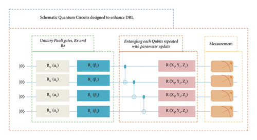
In the prototype of designed circuits shown in Figure 2, the agent is initially placed on the state |0000〉, and taking this encoded state as input, the unitary Pauli gates are applied to rotate the values on the arbitrary x-axis and z-axis. The entangling layer of the circuit entangles the values of unitary Pauli gates making the entangling between the qubits. The measurement layer measures each expectation value, which is related to the probability of measuring a certain state and how much does that state adds to the cost function.

3.4. Hybrid Classical-Quantum Deep Reinforcement Learning

The proposed hybrid framework with the designed VQC is viable on the existing noise intermediate scale quantum machine learning platform. Thanks to Xanadu for providing the PennyLane which consists of quantum machine learning libraries to simulate various tasks of quantum-enhanced machine learning, and the developed framework can resolve the VQC depth challenges by being hybridized with iterative parameter optimization (IPO) on a classical computer. Classical optimization takes place external to the quantum circuit and it provides the loss function and gradient calculations to update the parameters.

In our work, the loss function is calculated by mean squared error and RMsprop optimizers for providing an update for the parameters. Currently, PennyLane provides seven types of hardwired optimizers, which can work with the standard gradient descent with momentum, gradient descent, gradient descent with Nesterov momentum, Adam, Adagrad, and RMSprop. PyTorch and TensorFlow use optimizers that this library provides [33]. Here, we have selected RMSprop (the little explanation about the optimizers is found in T. Tieleman and G. Hinton, “Lecture 6.5_RmsProp: Divide the gradient by a running average of its recent magnitude”) which is broadly utilized in deep reinforcement learning. The parameter used in this optimizer is the learning rate, alpha, and eps which are applied for gradient descent optimizers (GDO) only. For the frozen lake environment, the utilized strategy for the ε-greedy is given by

$$ ()

From Figure 3, the experience replay chooses ε-greedy action from the current state, executes it in the frozen lake environment, and returns a reward and then moves to the next state. It keeps this observation as a training sample of data. All previous experience replay observations are kept as training data. We now take the random batch of samples from this training data, so that it comprises of a combination of older and more recent samples. This batch of training data is then entered into both the quantum Q network and the target quantum network. The quantum Q network takes a current state and an action from the separate data sample and predicts the quantum Q value for that specific action which then becomes the predicted quantum Q value.

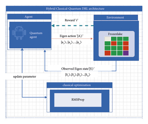
The target quantum network takes the next state from each data sample and predicts the best Q value out of all actions that can be taken from that state and is called the target quantum Q value. The predicted quantum Q value, target Q value, and the observed return of reward from the data sample are used to calculate the loss to train the quantum Q network. Moreover, we take a broad view of VQC to the standard deep reinforcement learning for approximating the action-value function. Lastly, we examine a policy reward of different hyperparameters of deep reinforcement learning for investigating the performance of PennyLane-based quantum deep Q-learning. For the testing environment, we have selected the standard openAI gym [43] frozen-lake environment.

Algorithm 1 Quantum enhanced DQL sampled from Huang [26] and Chen et al. [13].

Algorithm 1: Quantum enhanced deep Q-learning.
•  

  Set replay memory M to state size N

•  

  Initialize action-value function quantum circuit Q with arbitrary parameters θ

•  

  For episode e = 1, 2, 3, 4, ……. E do

•  

   Initialize State s1 from the set state S and encode it into

•  

   the quantum state using basis encoding

•  

   for the time step t = 1, 2, 3, …. T do

•  

    With probability ε, select a random action a_t

•  

    otherwise, select the optimal action at a_t = max_a  q_∗(s_t, a; θ) from the result of quantum circuit

•  

    Execute the selected action a_t and see the reward r_t and the next state s_t+1

•  

    Store transition (s_t, a_t, r_t, s_t+1) in replay memory M

•  

    Sample a random minibatch of transitions (s_b, a_b, r_b, s_b+1) from the replay memory M

•  

    $$

•  

    Perform a gradient descent step on $$

•  

   end for

•  

  end for

3.4.1. Action Selection in Quantum Enhanced Deep Q-Network

In deep reinforcement learning, the agent takes an action based on its policy. Selecting the best action among the other set of actions can provide a better reward for the agent. Here in the enhanced framework, selecting the action is determined via quantum expectation values of n number of quantum bits (Qubits). We have four action and four qubit systems which means that there are four expectation values after the measurement is applied on a four-qubit quantum system. Then, we represent each measurement of the qubit output wire (port) from zero to three. Then, the action with the index of the largest expectation value of the output wire is selected. For example, let us say our four qubit quantum system has the output wire with the set actions A = (a1, a2, a3, and a4). If the set of numerical expectation values of all actions after the measurement is e = (e (a1), e (a2), e (a3), and e (a4)) and the expectation value of e (a3) is greater than all four expectations, then the action that must be chosen is the index of action a3 which is 2. Now, action 2 is selected based on the expectation values and passed to the environment for testing. We recall that, in the FL environment, there are 4 actions in an agent’s action space. These actions are MoveTop, MoveDown, MoveLeft, and MoveRight, and their output wires of four-qubit quantum systems are indexed with 0, 1, 2, and 3, respectively. If the output of wire indexed with 3 has the greatest value of expectation, then the action that should be chosen by the quantum agent is to go up one stage from a current state in a frozen lake (FL). Quantum simulators such as PennyLane [44] and IBM Qiskit [45] are used to calculate the expected value of quantum measurements on the current classical computer. The result of expectation values after the quantum measurement is deterministic. Specifically, let us take the FL and let us say that the reinforcement learning quantum agent receives the state of 8 on the 4 × 4 grid which is 1000 in binary. The basis encoding with a two unitary Pauli gets are applied and this number must be converted to a quantum state such as |1〉 ⊗ |0〉 ⊗ |0〉 ⊗ |0〉. The encoded quantum state passes through the quantum circuit and at the end the expectation value will be measured. Here, the result after the measurement is either 0 or 1 if the system measures a first qubit |1〉 above, but the possibility of being 0 or 1 is stochastic or random. In random measurement, the agent selects only a single qubit randomly and uses that value for action selection. Each qubit of the prepared quantum state |1〉 ⊗ |0〉 ⊗ |0〉 ⊗ |0〉 can pass via blocks of the circuit and the measurement layer measure each qubit’s expectation value. For each qubit state, there are multiple number of repeated measurements but the chance of becoming exactly in the state |0〉 and state|1〉 is a probability distribution. This means that, we can predict the probability of being in state |0〉 and |1〉 by averaging the expectation value of repeated measurement. For example, let us measure T times the state of the first qubit |1〉 and from this measurement, if K times the state of some qubit gives 1, then the probability P(1)and P(0) is calculated as

$$ ()

The average value can be produced after the measurement, and this average value is called the value of quantum expectation.

To be specific, let us take the following example. The quantum agent again wants to measure the expectation value of |1〉 ⊗ |0〉 ⊗ |0〉 ⊗ |0〉 (See Table 3) and let us say that each qubit has been measured 500 times.

Table 3. The method of calculating the expectation value for action selection (this is the assumption).

	|1〉	|0〉	|0〉	|0〉
Total number of repeated measurements	500	500	500	500
Total number of measurements which gives 1	330	400	350	190
Total number of measurements which gives 0	170	100	150	310
Probability of getting 1 or P (1)	0.66	0.8	0.7	0.38
Probability of getting 0 or P (0)	0.34	0.2	0.3	0.62
Expectation value	0.66	0.8	0.7	0.62

Furthermore, each measurement on a quantum bit of n qubits can be executed concurrently in parallel.

4. Experimental Setup and Results

4.2. Experimental Result

The frozen lake environment is used in our work to evaluate the performance of DRL algorithms on quantum circuits. Previous practitioners such as Hu and Hu [14] used a grid-based environment similar to the frozen lake but with smaller size (2 × 3) grids. For this study, we have used the standard frozen lake values of grid size (4 × 4) by increasing the number of qubits to 4 which can have 2⁴ basis states. For the designed circuits, we have simulated numerically with the PennyLane [44]. A numeric simulator is used to discover the prospects of using quantum computing technology to solve DRL task and their optimality. To expand the former work of Hu and Hu [14], we present algorithms that improve upon the previous results. We have applied the learning techniques to OpenAI Gym [43] and frozen lake environments which are more complex with the number of states and layers than in the previous work [14]. To verify the trainability of the framework, we take 1000 episodes of the standard frozen lake experiment. The horizontal coordinate signifies an episode in the enhanced learning process, and the vertical axis represents the number of rewards returned to the agent for taking some actions on the environment. The experiment considers the trainability of enhanced DRL and the effect of the number of layers on the enhanced DRL framework. According to the experiment, the quantum enhanced DRL is trainable in all cases but, the time it takes to converge to the optimal value is different for the different quantum layers.

Figures 4(a)–4(c) show the learning ability of different quantum agents based on the different layers. From Figure 4(a), it is seen that the agent executed with two layers hit the maximum negative reward of −15.09 on episode 148. The agent tried and converges to the optimal Q value by taking the reward of 0.91 after the training episode of 525. The second agent from Figure 4(b) is executed with 3 layers and converges to the Q value with a total reward of 0.95 after the 397th episode. The third agent is executed with 5 layers and converges to the optimal Q-value with the reward of 0.95 after the 72^nd episode. Here we can conclude that, on the framework, the agent explores more if the framework uses a smaller number of layers and this means that, it exploits the optimal value when more layers are used. This means, when the quantum layer increases from 2 to 5, the framework converges faster without going for testing on various episodes. In the other scenario, the QDRL is better than classical DRL to reduce the parameters (weights in the classical case). Here, a number of parameters in PQC subjected to optimization can be calculated as

$$ ()

where θ is the number of quantum layers, the number of circuit blocks used in this research study is 3, and the +1 is the added bias which is also subjected to optimizations [13]. Classically, four layers of NN which need 16 x 4 or 64 parameters are needed to represent the 4x  4 frozen lake problem [13]. In QDRL, we can represent this problem with 4x(3 x 4 + 1) or 52 parameters which reduces the number of parameters by 12. So, QDRL is a better choice for parameter reduction. On the other hand, the quantum-enhanced action selection strategy makes a good balance between exploration and exploitation using expectation values, which increases the quantum agent learning ability and promises to solve searching problems over entire state-action (s and a) space search in classical DRL.

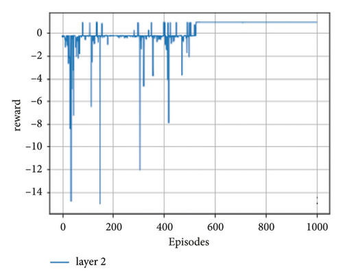
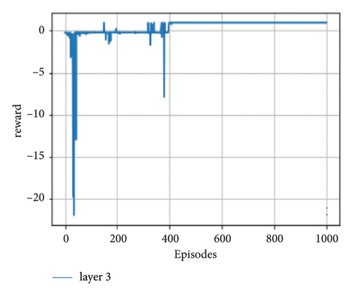
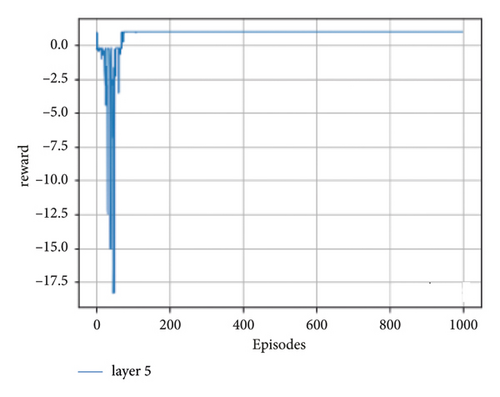
In the case of seeing the performance in different learning rates (alpha), the agent running with 0.1 alpha value hits the maximum time steps of 2012. When the alpha value is 0.1 or smaller, the agent explores much more but it learns very slowly, so the training process converges to the optimal state very slowly.

Figure 5 gives a precise description of enhanced framework learning results. We record every single learning epoch to verify the outcomes of enhanced DRL algorithms with selected 0.1, 0.2, 0.3, and 0.4 learning rates or alpha values (see Figures 5(a)–5(d), respectively). From this result, we can conclude that the greater the learning rate values in quantum deep reinforcement learning, the fewer timesteps it takes to move from the start point to the goal state. The result of QDRL shows advantages with 0.4 learning rate or alpha values. The advantages are the use of quantum representation. The quantum representation uses the quantum superposition strategies of quantum mechanics in which the updating method is carried out via quantum parallelism. Quantum parallelism will be more useful in the near future when quantum enhanced device comes into use rather than simulating on conventional computers.

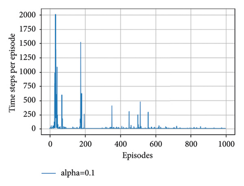
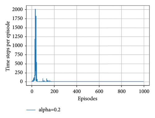
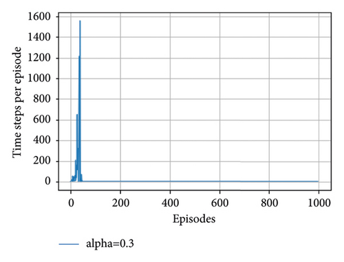
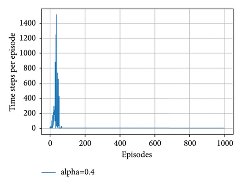
From Table 7, we can see that when the agent got the reward of 0.95, it costs the agent 6 timesteps which is the time step the agent takes to converge into the optimal state. Generally, the time steps of an agent with a learning rate from 0.2 to 0.4 for the last 200 episodes is similar which is 6 and the reward also converges to the optimal value of 0.95.

Table 7. The reward and timestep of the agent for the last 200 episodes.

Episode	799	849	899	949	999	Alpha
Reward	−0.24	−0.24	−0.26	0.95	0.95	←0.1
	0.95	0.95	0.95	0.95	0.95	←0.2
	0.95	0.95	0.95	0.95	0.95	←0.3
	0.95	0.95	0.95	0.95	0.95	←0.4
Timesteps	8	8	7	6	6	←0.1
	6	6	6	6	6	←0.2
	6	6	6	6	6	←0.3
	6	6	6	6	6	←0.4

5. Conclusions

Though the main focus of this study is enhancing DRL with quantum machine learning and analyzing the learning performance of that framework, we have studied the background of this technology and its applicability as well as and the need of applying this technology to current machine learning models. This can be seen from two sides which are the theoretical side and the technical side. On behalf of the theoretical study, we have studied that, the motivation behind this new machine learning paradigm is to obtain improved learning performance. The study also presents the state-of-the-art in the development of quantum science in the area of AI and encourages the enhancement of classical ML technology. Specifically, the representation of quantum computations is generally different from the current classical computations, and various features of quantum computation are prospectively evolving.

Machine learning is a feature that is currently influenced by the theory of quantum computation. There are various demonstrations and conformations that quantum mechanical phenomena such as superposition, entanglement, and quantum inference which can change the current machine learning algorithm such as supervised, unsupervised, and reinforcement learning for its betterment in providing sustainable speed up on processing data. In this study, we also analyzed the need for classical data and the method of encoding it to the quantum state to process it on cloud-based provided resources of quantum machine learning. To be accessed and processed on quantum processing units, the data need to be encoded into the quantum state. The type of encoding can be different from task to task for the specific problem that needs to be solved.

Generally, we have analyzed that knowing the encoding techniques that can handle the problems with that limited resource is expected from the researcher as the existing quantum devices are very small and intermediate scale. They only cover a small number of qubits. The other thing is considering the complexity of circuits. Minimizing the number of quantum circuits is needed to reduce the complexity and needs to minimize the number of parallel quantum actions required to grasp the quantum encoding. The well-known quantum data encoding is computational basis encoding which provides codification of classical data to a quantum state. Quantum phenomena such as superposition and entanglement can provide parallelization for all quantized states. Lastly, we have confirmed that the computational basis encoding is not efficient for the quantum deep reinforcement learning (QDRL) problem that needs a huge number of qubits but is efficient for tasks solved by applying a smaller number of qubits. The standard DRL task can be enhanced with a smaller number of qubits because the trainability of the framework can be investigated on a standard frozen lake which contains 4 × 4 matrices of state action spaces.

On behalf of the practical side, the outcomes of experiments validate the feasibility of an enhanced deep Q-learning framework and then verify its learning performance for the agent with different quantum layers and different learning rates. The experiment depicts that the value of a number of layers and the number of learning rates can affect the learning performance of an agent and as soon as a quantum-enhanced deep reinforcement learning turn on a real quantum computer, it can be efficiently used to improve the quantum robot learning for achieving some important tasks. Generally, we have verified the applicability of quantum computation to machine learning specifically deep reinforcement learning, and the further exciting results are what we expect after this enhanced deep Q-learning run on fully quantum computers in the nearby future.

6. Recommendations

Quantum-enhanced machine learning as a whole and quantum-enhanced deep reinforcement as specific is a newly quantum computing-inspired learning framework that has a theoretical and experimental gap. Most of the experimental gaps can be solved only when the quantum resource is available than today’s resources. Most companies such as IBM, Google, and Xanadu are trying to handle these problems by providing cloud-based resources. Though the resource is enough for some simple problems, it is not efficient for complex problems such as the Atari games and Game of Go. Here, every activity such as state representation (preparation and encoding), policy evaluation and policy iteration, action selection, and optimization in reinforcement learning needs theoretical and experimental studies to enhance it with quantum computing technology. In the case of state representation, we have applied basis encoding techniques to encode the classical states into quantum states and we recommend that, by seeing the framework’s performance applying other encoding techniques such as amplitude and angle encoding. In this paper, we mostly discussed the deep reinforcement problem with discrete state spaces. But the expected recommendation here is to extend this enhanced framework to DRL problems with continuous state spaces efficiently.

Conflicts of Interest

The authors declare that they have no conflicts of interest.