The complexity and high dimensions of big data sonar, as well as the unavoidable presence of unwanted signals such as noise, clutter, and reverberation in the environment of sonar propagation, have made the classification of big data sonar one of the most interesting and applicable topics for active researchers in this field. This paper proposes the use of the Grasshopper Optimization Algorithm (GOA) to train Multilayer Perceptron Artificial Neural Network (MLP-NN) and also to select optimal features in big data sonar (called GMLP-GOA). GMLP-GOA hybrid classifier first extracts the features of experimental sonar data using MFCC. Then, the most optimal features are selected using GOA. In the last step, MLP-NN trained with GOA is used to classify big data sonar. To evaluate the performance of GMLP-GOA, this classifier is compared with MLP-GOA, MLP-GWO, MLP-PSO, MLP-ACO, and MLP-GSA classifiers in terms of classification rate, convergence rate, local optimization avoidance power, and processing time. The results indicated that GMLP-GOA achieved a classification rate of 98.12% in a processing time of 3.14 s.

1. Introduction

Nowadays, big data analysis and classification are highly valuable [1, 2]. The reason is that as the data increase, the need for more accurate data analysis and classification also increases [3, 4]. The more precise and accurate analysis, the more secure our decision-making will be. Better decisions mean more practicality and less cost. Sonar data is one type of data that is regarded to be part of the big data family [5, 6].

Concerning the complex physical characteristics of sonar purposes, classifying original purposes and avoiding unreal purposes has developed into a critical practical area for active researchers and craftsmen [7, 8]. Due to the complexity and heterogeneity of sound circulation in saltwater, several parameters for categorization and differentiation of sonar purposes should be extracted. As the dimensions of the feature vectors grow, the data dimensions also grow.

There are two distinct ways of categorizing high-dimensional data [9]. The first is to employ the Deterministic Approach [10]. Because this approach is so reliable, it almost always results in the best response; nonetheless, the method encounters difficulties as data dimensions rise, which is followed by an increase in spatial and temporal complexity [11]. Furthermore, this strategy is inapplicable to the data classified as big data [12, 13]. The stochastic method is the second approach [14]. These methodologies yield a near-optimal solution [15]. Additionally, they are less complicated in terms of spatial and temporal dimensions than deterministic methods [16, 17]. Artificial Neural Networks (ANN) is one of the most effective stochastic methods utilized in the actual world of big data.

Neural networks have the ability to learn [18]. Learning here means, these networks are the basics of all neural networks, which may be parted into two groups of supervision learning [19] and without supervision learning [20, 21]. Most appliances are optimized for Multilayer Artificial Neural Networks, optimized [22] or standard [10, 23]. Backpropagation algorithm is used as a learning method that is considered among the family of supervised learning. The backpropagation algorithm is on an incline basis which has some problems such as gradual convergence [24] and appliance in a limit area [25, 26]. Thus, they are unreliable for functional appliances.

The eventual purpose for the process of learning in neural networks is to acquire the best structure of weighted edges and their bios. Such a way that the least number of errors may occur in network training and test specimens [27, 28]. The reference [29] demonstrates that metaheuristic optimization methods may be substituted with gradient-based learning algorithms, since the stochastic character of these algorithms prevents them from being trapped in a local optimum, increases the convergence rate, and decreases classification errors.

Some of the metaheuristic methods which have been recently used for training neural networks, are genetic algorithm (GA) [30], simulated annealing (SA) [31], biogeography-based optimization (BBO) [32], Magnetic Optimization Algorithm (MOA) [33], Artificial Bee Colony Algorithm (ABC) [34], Gray Wolf Optimizer (GWO) [35], Social Spider Algorithm (SSA) [36, 37], Particle Swarm Optimization and Gravity Search Algorithm (PSOGSA) [7], and so on. GA and SA decrease the possibility of getting stuck in the local optimum, but their low convergence rate. This shortage leads to a weak performance when the need for an immediate process exists. ABC acts properly dealing with small problems and data with low dimensions, but when the problem dimensions increase, the time for training increases greatly as well. MOA has an unsuitable performance and low accuracy, facing nonlinear data. BBO requires lengthy computations. Despite its simplicity and speed of convergence, GWO becomes trapped in the local optimum and so is not ideal for situations with a global optimization. Numerous adjustment parameters and a high level of complexity are SSA’s flaws. PSOGSA is formed by a combination of PSO and GSA which leads to an increase in the spatial and temporal complexity.

One of the commonalities between metaheuristic algorithms and other search algorithms is the split of the search region into two phases: exploration and exploitation [38–40]. The first phase occurs concurrently with the algorithm’s attempt to examine the most dependable areas of the search region [15, 41]. During the exploration phase, the population is subjected to abrupt alterations in order to properly investigate the whole region of the problem. The exploitation phase happens when the algorithm is converged toward a reliable answer. At this stage, the population is undergoing very small changes.

In most cases, given the random nature of evolutionary algorithms, there is no specified boundary betwixt these 2 phases [18, 42]. In other words, the lack of balance betwixt these two phases causes the algorithm to get stuck in the local optimum. This problem is intensified, dealing with data with high dimensions. By adjusting the displacement behavior betwixt these 2 phases, the probability of getting stuck in the local optimum can be reduced. As proved in the reference [43], GOA can properly recognize the border between exploration and exploitation phases [44, 45]. Thus, the algorithm converges toward more reliable answers.

On the other hand, any system that performs data classification consists of three main parts: data acquisition, feature extraction, and classifier design. The novelty of this article occurred in the feature extraction section. In general, all extracted features are not useful and may contain useless or duplicate information. Feature selection can be seen as the process of identifying useful features and removing useless and repetitive features. The goal of feature selection is to obtain a subset of features that solve problems well with minimal performance degradation. The goal of feature selection is to obtain a subset of features that solve problems well with minimal performance degradation.

This theory is mentioned here: No Free Lunch (NFL) [46, 47]. This proposition demonstrates logically that no metaheuristic method exists that is capable of resolving all optimization problems. In other words, one metaheuristic technique may perform admirably and predictably on one set of issues while failing miserably on another set of problems [48, 49]. NFL stimulates this field of study and contributes to the development of new methodologies and the formulation of new metaheuristic methods on an annual basis [50]. Taking into mind the described theory, the aforementioned issues, and GOA’s capacity to cope with big data, this approach may be utilized to train Multilayer Perceptron Neural Networks (MLP-NN) and, subsequently, to classify sonar data.

On the other hand, any system that performs data classification consists of three main parts: data acquisition, feature extraction, and classifier design. The novelty of this article occurred in the feature extraction section. In general, all extracted features are not useful and may contain useless or duplicate information. Feature selection can be seen as the process of identifying useful features and removing useless and repetitive features. The goal of feature selection is to obtain a subset of features that solve problems well with minimal performance degradation. The NFL theorem and the ability of GOA to find the boundary between the two phases of exploration and extraction in the search space is a strong motivation to investigate GOA for the problem of feature selection. Therefore, in this paper, in addition to GOA being used as a neural network training algorithm, GOA is used to select optimal features (GMLP-GOA).

The main contribution of this paper is as follows:

(i)
Obtaining and collecting experimental data sets
(ii)
Feature extraction using the MFCC method
(iii)
Feature selection using GOA
(iv)
Designing an optimal GMLP-GOA hybrid classifier and classification of big data sonar
(v)
Data classification using MLPs trained with five population-based metaheuristic algorithms

This paper is organized as section two will introduce the MLP-NN. Section 3 explains general issues for GOA. Section 4 will describe how the outcoming GOA as a training algorithm for metaheuristic methods in MLP-NNs is applied. Section 5 will present the dataset and feature selection. Section 6 presents experimental results and discussion. References used are provided in Section 7.

2. Multilayer Perceptron Neural Network

Figure 1 displays an MLP-NN where m, l, and s, respectively, stand for the number of input nodes, hidden nodes, and output nodes [51, 52]. As observed, there is a one-sided junction betwixt the nodes of MLP-NN, which is among the group of neural networks (FNN) [53, 54]. MLP-NN output is computed by

(1)

Details are in the caption following the image — Open in figure viewer PowerPoint

In this relation W_ij stands for the weight of the edge which connects i-th node (input layer) to j-th node (hidden layer), X_i stands for the input to i-th node (input layer), θ_j stands for the bios of j-th node (hidden layer), and m stands for the number of input nodes. Any hidden node’s output is acquired as a relation (2) to a sigmoid function.

(2)

(3)

(4)

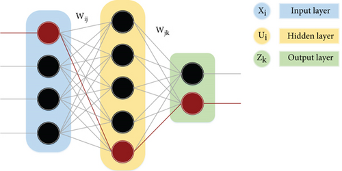
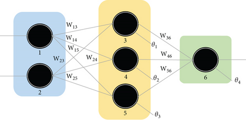
After calculating the hidden nodes, it is possible to define the final outputs as follows.

In which W_jk stands for the weight of the edge which stands for the bios of the node k -th and connects the node j −th (hidden layer) to the node k −th (output layer). The most essential factors of an MLP-NN, are the weight for edges and their bios. As seen in the above relations, edges weigh, and bios have defined the ultimate output. Training an MLP-NN, consist of detecting the best optimal output out of certain outputs.

3. Grasshopper Optimization Algorithm

Grasshoppers are an insect species. They are classified as pestilences owing to the harm they do to agricultural crops [55–57]. Although grasshoppers seem to be alone in nature, they are part of one of the biggest animal groups on the planet. They, sometimes, are a threat to farmers. One of their unique features is their social behavior which can be seen both in their childhood and their maturity. Millions of their kids jump and roll-like rollers and eat almost all the plants along the way. Slow movements and short steps are the main features of grasshoppers. Short and sudden movement is one feature of a mature grasshopper community. An important feature of their community is the search for food resources [58]. GOA being inspired by nature, logically, divides the searching process into 2 phases of exploration, and exploitation.

While seeking agents are encouraged to make abrupt moves during the exploration phase, they prefer to make local movements during the exploitation phase. The mathematical model for simulating this grasshopper social behavior is as follows [43]:

(5)

where X_i is the location of the i -th grasshopper, A_i denotes the wind, S_i denotes social interaction, and G_i denotes the gravity placed on the i -th grasshopper. To include randomness, the equation is modified as follows:

(6)

where r₁, r₂ and r₃ are random numbers between [0,1].

(7)

where d_ij is the distance between the i-th and j-th grasshoppers and is calculated using the relationship (8). S is a function that is used to define social power. As seen in equation (9) and in the relationship below,

is a unit vector extending from the i-th grasshopper to the j-th grasshopper.

(8)

The function s shows social power as follows:

(9)

f is the intensity of absorption and l is absorption length scale. The function S is not able to impose strong powers between faraway grasshoppers. The G component of the relation (6) is computed as follows:

(10)

where g denotes the gravitational constant and

denotes a unit vector pointing toward the earth’s center. Component A in relation (1) is obtained by

(11)

where u denotes a constant displacement and

denotes a unit vector perpendicular to the wind direction.

Because grasshopper larvae lack wings, their motions are entirely dependent on the direction of the wind. After placing S and G values in the equation (1), this equation can be expanded as

(12)

where the relation (9) and N are equal to the number of grasshoppers. Their children’s location on the ground should not be lower than the threshold. We will not, however, utilize this equation to simulate the grasshopper group and the optimization algorithm in order to prevent the algorithm from exploring and exploiting the search space around the solutions. The mathematical model is capable of simulating the grasshopper community in 2- and 3-dimensional as well as multidimensional spaces. However, this mathematical model cannot directly be used for solving optimization problems. The main reason for this is the rapid growth of grasshopper in the area of inertia. As a result, this group cannot converge on a single point. A reformed version of this equation is presented as follows for the purpose of addressing optimization problems:

(13)

where ub_d is the upper limit on the d dimension, lb_dis the purpose value of the d dimention (the best answer so far). Relation (9) and also

is a constant decreasing coefficient to reduce the area of inertia, absorption, and desorption. It should be considered that S is almost similar to S in the relation (1). However, we disregard the linear trend and assume that the wind component is always ideal (purpose value).

Equation (13) demonstrates that the position of the grasshopper is determined in terms of its present location, the position of the best solution, and the position of all grasshoppers in the group. It is worth noting that the first component of this equation examines the current location of the grasshopper in relation to the positions of other grasshoppers. To determine the placement of search agents around the purpose, we assessed the state of all grasshopper positions. This is in contrast to the particle swarm algorithm. Each particle in the particle mass algorithm has two vectors: a location vector and a velocity vector.

However, in the grasshopper algorithm, each search agent is represented by a single vector. Another significant distinction between the two methods is that the particle swarm algorithm modifies its location depending on the particle’s current position, the particle’s best position, and the group’s best response. Whereas in the Grasshopper Algorithm, the location of the search agent is modified based on its current position, the best response, and the positions of all the particles in the group. This implies that none of the other groups in the particle swarm algorithm engage in updating a particle’s location, but the Grasshopper Algorithm needs all search agents to participate in deciding each agent’s next position.

The parameter C is utilized twice in equation (13) for the following reasons. The first C on the left is fairly similar to the particle swarm algorithm’s (w) weighted inertia. This setting reduces the grasshoppers’ movements in the vicinity of the objective spot. In other words, this parameter optimizes the balance between the exploration (search) and exploitation stages of the input population. The second parameter in the equation decreases grasshopper absorption, inertia, and desorption. Consider the component in the equation (13), the component c(ub_d − lb_d)/2 linearly reduces the space that grasshoppers should explore and exploit. The component s (x_j − x_i)/d_ij indicates the grasshopper’s absorption to the purpose or the grasshopper’s desorption from the optimal location.

Internal C decreases absorption and desorption forces among grasshoppers as the number of repetitions increases, but external C decreases the coverage area around the ideal response as the number of repetitions increases. In summary, the first statement of equation (13) takes into account the total of the positions of the other grasshoppers and applies the grasshoppers’ natural interaction. replicates the grasshoppers’ hunger for food in the second sentence. Additionally, parameter C replicates the decline in the grasshoppers’ acceleration to and intake of the food source. To increase the randomness of the behavior and as a substitute, both phrases of equations (13) might be multiplied by a random value. Single sentences can also be multiplied by random values to model the grasshopper’s random behavior in interaction with each other as well as the tendency toward the food source. The mathematical approach offered here is capable of exploring and exploiting the search space. However, a mechanism must exist to transition candidates from the exploration stage to the exploitation stage. Naturally, grasshoppers look for food locally initially, since they lack wings throughout their infancy. They then fly freely across the air, discovering new regions. Unlike this, in stochastic optimization techniques, the exploration phase is conducted first to determine the permissible regions of the search space. Following the discovery of permitted areas, the exploitation phase forces the search agents to locate an accurate approximation of the optimal answer location on a local level.

To balance the two phases of exploration and operation, parameter C must be reduced according to the number of repetitions. This mechanism increases efficiency when the number of repetitions increases. The area of inertia is reduced in proportion to the number of repetitions and is computed as follows:

(14)

where cmax is the maximum value, cmin is the minimum value, l is the current repetition count, and L is the maximum repetition count. These parameters were assigned values of 1 and 0.00001 in this study. The appropriate purpose chase by the group is due to the effect of the last sentence of equation (12) that the grasshoppers tend to be attracted to the purpose value. The more interesting pattern is the gradual convergence of the grasshoppers toward the purpose with increasing repetition, which is again due to the decrease in the parameter C. This behavior helps the GOA algorithm not to quickly converge to the optimal answer and thus not get stuck in the local optimal. Therefore, in the latter phases of optimization, the grasshoppers approach as closely as possible to the objective, which is important in the exploitation space.

The preceding discussion demonstrates that the suggested mathematical model motivates grasshoppers to progress toward the goal with increasing repetitions. However, in a true search space, there are no objectives, since it is not quite evident what the best and most significant objective is. As a result, each optimization phase requires us to assign a purpose to each collection of grasshoppers. The Grasshopper Algorithm makes the assumption that the best or purpose value is the most suitable grasshopper (response vector) throughout the optimization process. This will help the algorithm store the most appropriate answer vector in each repetition and in the search space and direct the grasshopper group toward that purpose value. This is done in the goal of discovering a more precise and superior purpose that serves as the best approximation for the overall and true optimization of the search space.

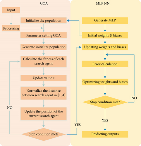
The Grasshopper Algorithm flowchart utilized in the neural network is seen in Figure 2. The GOA method begins by generating a random beginning population. Agents of search revise their positions in light of connections (13). Each iteration has updated the best answer so far. Additionally, factor c is determined using equation (14), and the distance between grasshoppers is normalized to a value between one and four. Updating the grasshopper position has been repeatedly performed to reach the criterion of terminating the algorithm. The position and value of the objective function of the optimal answer, as the best approximation of the overall optimal answer, is finally obtained.

4. Training a Multilayer Neural Network Using the Grasshopper Algorithm

In general, there are three ways for training MLP-NN using evolutionary algorithms. The first is to utilize evolutionary networks to determine the optimal mix of edge weight and node bias in an MLP-NN. The second is the use of evolutionary networks to determine the optimal arrangement of MLP-NNs in a given situation, and the third is the use of evolutionary networks to determine the learning rate and amount of movement of the gradient-based learning algorithm. The Grasshopper Optimization Algorithm is evaluated against an MLP-NN utilizing the 1-th approach in this research. To appropriately represent the weights of edges and nodes in a training procedure for MLP-NN networks, the weights of edges and nodes must be properly represented.

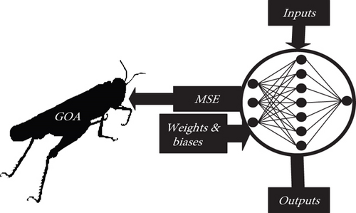
Generally, three methods are used to express the weight of edges and the bias of nodes: vector, matrix, and binary. Each element is represented as a vector, matrix, or string of binary bits in the vector, matrix, and binary methods. Each of these strategies has a number of benefits and downsides that may be advantageous in certain situations. Figure 3 shows how to train a neural network using GOA.

While it is straightforward to convert elements to vectors, matrices, or strings of binary bits using the first technique, the process of retrieving them is more complex. As a result, this technique is often utilized in rudimentary neural networks. In the second technique, it is simpler to recover than it is to encode components in complicated networks. This approach is particularly well-suited for developing algorithms for generic neural networks. The variables must be supplied in binary form for the third technique. When the network structure becomes intricate in this item, the length of each element likewise increases. As a result, the coding and decoding processes will be very difficult.

In this paper, since we do not deal with complex multilayer neural networks, the vector method is used. The MATLAB generic toolbox will not be used to reduce the time of the multilayer neural network operation. As an example of this coding method, the final vector of the multilayer neural network shown in Figure 4 is given in.

(15)

5. Data Set

This chapter uses one of the most challenging engineering problems in the real world to prove GOA’s capability. The chosen issue is the classification of sonar data, which is one of the challenges and concerns of engineers and scientists, working in this field.

5.1. Scenario Test Design and Experimental Data Formation

Since our goal is to obtain a reliable and realistic set of high-dimensional sonar data, a real experiment was designed and implemented. The experiment was conducted using the tunnel cavitation model NA-10, made in England. In the first phase, three types of impellers were produced in classes A, B, and C. The Class A impeller has three blades that can be used to pick up sound from a boat, and small passenger ship. The Class B impeller has four blades that are used to get the sound from a container ship, ocean liner, and small oil tanker. The Class C impeller has five blades and is used to extract sound from the aircraft carrier and large oil tanker. In this experiment, the impellers are evaluated at different speeds to simulate different operating conditions. During these experiments, the sound (acoustic noise) of the various impellers was stored on a computer using the B&K 8103 hydrophone and Data-Logger of the UDAQ_Lite model.

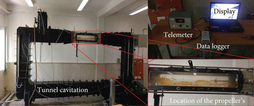
The proposed test scenario is shown in Figure 5. Propulsion velocity in free water is expressed as a number without J dimension, proportional to rotation speed N(RPM) or rotation speed per second (RPS) and impeller diameter D (m) and v the water flow velocity:

(16)

At all experiments, the atmospheric pressure of 100 kPa and pressure inside the tunnel were considered concerning the depth of impeller placement in that floating class. The water flow rate inside the tunnel is also 4 m/s. One of the hydrophones is mounted next to the propeller at a distance of 10 cm and the other 50 cm from the first hydrophone.

In this section, the noise of the designed impellers is measured in four steps. In the first step, after the water flow slows down, the noise is received by the hydrophones and then received and stored by the MATLAB software and Data-Logger. Secondly, by turning on the impeller and without the impeller wheel, the engine noise is also obtained in several stages, so that we can obtain a reasonable estimate of this noise. In the third stage, the impeller rotates at different rotations (depending on the type of the model float) to obtain the impeller rotation noises for the different floating classes. In the fourth step, by turning on the water rotation pump and the bubble discharging pump into the discharge tunnel, the impeller motor is activated and the sound is collected by the Data-Logger and the MATLAB software, in the computer. At all stages, all the actual data, without amplifying the values, are stored in the computer for later use.

5.1.1. Drawing Noise Curves for Model propeller’s

According to the standard reference [30, 31] the power is calculated in dB related to the water acoustic reference power (1μPa). Figure 6 shows noise curves at the hydrophone surface, Fourier transforms, and dB power spectrum, respectively, for different classes of impellers.

Generally, the relation (17) is used to obtain the fundamental frequency by RPM.

(17)

In this section, 500 samples with different propeller and a number of rotations were obtained.

5.2. Feature Extraction

After the preprocessing section after receiving the detected frames containing the audio matching to the received signals, the detected sounds are provided to the feature extraction section with the effects of synthetic phenomena eliminated and converted to the frequency domain (called S (k)). At this point, the signal spectrum’s energy is calculated using the following;

(18)

S_r(k) and S_i(k) denote the real and imaginary components of the detected signal’s Fourier transform, respectively. After that, Mel-scaled triangle filters are used to filter the spectral energy of |S(k)|². The relationship between the output energy of the l filter and (20).

(19)

N is the number of discrete frequencies utilized in the FFT conversion of the preprocessing phase, and H_l(k) is a filtered transfer functions, where l = 0. The logarithm function compresses the dynamic range of the Mel-Filtered Energy Spectrum.

(20)

Eventually, the relation (21) and discrete cosine transform are used to convert the Mel-Frequency Cepstral Coefficients (MFCC) to the time domain (DCT).

(21)

The feature vector will be as the relation in this situation and for any explicit purpose.

(22)

Figure 7 shows a block diagram of the procedures involved in the classification steps.

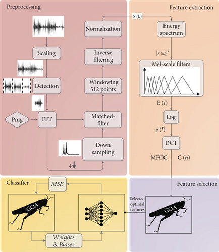
This section contains 140 extracted characteristics. Given 500 samples, the data set will be 500 × 140 in size, with 140 representing the number of input nodes (n) in the neural network and 281 being the number of neurons in the hidden layer. Thus, despite the vast data sets, computational and deterministic approaches have a high time complexity, and random methods are regarded as the optimal answer for this kind of problem.

5.3. Feature Extraction

As discussed in the previous subsection, the dimension of the feature matrix is 500 × 140. All extracted features are not useful and may contain useless or duplicate information. As shown in Table 1, there are 2¹⁴⁰ states for the obtained feature matrix. The binary version of GOA is responsible for selecting the optimal features.

1. Different feature modes.

Feature vector states	f₁	f₂	f₃	⋯	f₁₃₈	f₁₃₉	f₁₄₀
1	0	0	0	⋯	0	0	0
2	1	0	0	⋯	0	0	0
3	1	1	0	⋯	0	0	0
4	1	1	1	⋯	0	0	0
⋮	⋮	⋮	⋮	⋮	⋮	⋮	⋮
2¹⁴⁰-2	1	1	1	⋯	1	0	0
2¹⁴⁰-1	1	1	1	⋯	1	1	0
2¹⁴⁰	1	1	1	⋯	1	1	1

It is assumed that the initial population is 209. Table 2 shows the hypothetical values for the initial population of 209.

2. Assumed values for an initial population of 209.

Initial population	f₁	f₂	f₃	⋯	f₁₃₈	f₁₃₉	f₁₄₀
1	0	1	0	⋯	0	0	0
2	0	0	1	⋯	0	1	0
3	1	0	0	⋯	0	1	1
⋮	⋮	⋮	⋮	⋮	⋮	⋮	⋮
207	0	0	0	⋯	1	0	1
208	1	1	1	⋯	0	1	0
209	1	0	1	⋯	0	0	1

In Table 2, each row is used as a feature selection pattern. By using these patterns, the entire educational input data is selected. In this paper, accuracy is used as a fitness function. In the following, MLP-GOA is used to calculate the fitness function. Therefore, for each selected pattern, the accuracy is calculated using MLP-GOA (the accuracy value is exactly the fit value of each pattern). Assuming that the initial population is 209, the length of the fitness vector will also be equal to 209. Figure 8 shows how to select the feature from the most optimal selection pattern.

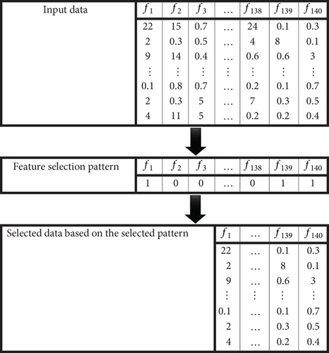
If the stop condition (reaching 100% accuracy or reaching the maximum number of iterations) occurs, the program ends, and the data in the best pattern (selected and reduced features) is selected for classification with MLP-GOA.

6. Experimental Results and Discussion

For fair comparison and performance evaluation of GMLP-GOA classifier, five classifiers MLP-GOA, MLP-GWO, MLP-PSO, MLP-ACO, and MLP-GSA are used. The selection algorithms are all population based. GMLP-GOA and MLP-GOA classifiers have the same training by GOA. The only difference between these two classifiers is that in the GMLP-GOA classifier, GOA is used for feature selection. Table 3 contains the parameters and beginning values for these algorithms.

3. Parameters and initial values of training algorithms.

Algorithm	Parameter	Value
GWO	Population size	209
GWO	The number of Gray Wolf	13

PSO	Population size	208
	Cognitive constant (C1)	1.1
	Social constant (C2)	1.1
	Local constant (W)	0.4

ACO	Population size	209
	ACO primary pheromone (τ0)	0.000001
	Pheromone updating constant (Q)	20
	Pheromone constant (q0)	1.1
	Decreasing rate of the overall pheromone (Pg)	0.8
	Decreasing rate of local pheromone (Pt)	0.6
	Pheromone sensitivity (a)	2
	Observable sensitivity (β)	6

GSA	Population size	209
	Coefficient (α)	21
	Limit down	-31
	Limit up	31
	Gravitational constant (G°)	1
	The initial speed of the masses	[0, 1]
	The initial value of the acceleration	0
	The initial value of mass	0

GOA	Population size	209
	Highest value (cmax)	1
	Lowest value (cmin)	0.00001

In the GMLP-GOA hybrid classifier, the optimal features obtained from GOA are used. If for other classifiers, a feature matrix with dimensions of 500 × 140 is used. Classifiers are evaluated in terms of classification rate, local minimization avoidance and convergence speed.

Table 4 shown the classification rate, mean and standard deviation of the smallest error, and P value for each method after it has been run 20 times. The classification rate indicates the correct recognition accuracy of the classifier, while the smallest error’s mean values and standard deviation, as well as the P value, and show the algorithmic power in avoiding local optimization. Also shown in Figure 9, is a comprehensive comparison of the convergence rate and method and the final error of the classifiers.

4. Results of applying different training algorithms in designing sonar purpose classifier.

Classifier	MSE (AVE ± STD)	P values	Classification rate (%)	Processing time (s)
GMLP-GOA	0.1055 ± 3.4180e − 01	N/A	98.1276	3.14
MLP-GOA	0.1283 ± 8.2720e − 04	N/A	95.6667	6.24
MLP-GWO	0.1519 ± 0.0269	0.0039	94.3522	7.39
MLP-GSA	0.3149 ± 0.2965	6.2149e-04	69.6633	10.44
MLP-ACO	0.2527 ± 0.1744	7.2798e-12	75.3333	7.54
MLP-PSO	0.2011 ± 0.2076	0.2239e-03	92.8222	8.78

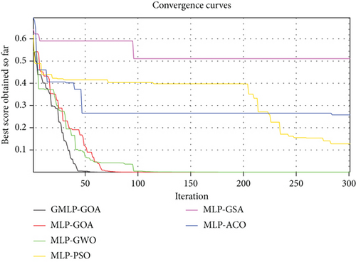
As shown in Figure 9, GMLP-GOA has the best convergence rate and MLP-GSA has the worst convergence rate among the used classifiers. The results obtained in Table 4 show that in terms of classification rate, GMLP-GOA succeeded in classifying sonar big data with 98.12% accuracy, while MLP-GSA had the worst performance with a classification rate of 69.66%. In terms of processing time, GMLP-GOA had the fastest processing time with 3.14 s, while MLP-GSA required more time for processing than other classifiers with 10.44 s. As can be seen in Table 4 and the values of standard deviation and P value, the GMLP-GOA hybrid classifier performs optimally in terms of avoiding being trapped in the local minimum. One of the reasons for the success of GMLP-GOA can be mentioned the power of GOA in detecting the boundary between exploration and extraction phase. As shown in Figure 9, GMLP-GOA converged after 50 iterations, while MLP-GOA and MLP-GWO converged after 75 and 95 iterations, respectively. Therefore, according to the obtained results, GMLP-GOA showed a successful performance in dealing with sonar big data and is recommended for use in real-world problems.

7. Conclusion

In this paper, GOA is used to select optimal features and train MLP-NN in GMLP-GOA hybrid classifier to classify sonar big data. Also, to have a fair comparison, 5 classifiers MLP-GOA, MLP-GWO, MLP-PSO, MLP-ACO, and MLP-GSA were used, which are all based on population-based metaheuristic algorithms. As seen in the simulation results, GOA can correctly detect the boundary between exploration and exploitation phases. Therefore, it does not get stuck in local optima, and its ability to find global optima for solving high-dimensional problems such as big data sonar is well-proven. The results show that GMLP-GOA has the best performance for classifying sonar big data by reaching a classification rate of 98.12%. 5 classifiers MLP-GOA, MLP-GWO, MLP-PSO, MLP-ACO, and MLP-GSA have the most accurate classification accuracy by reaching values of 95.66, 94.35, 92.82, 75.33, and 69.66, respectively.

Conflicts of Interest

The authors declare that they have no conflicts of interest.

Open Research

Data Availability

No data were used to support this study.

References

1 He R., Ai B., Molisch A. F., Stuber G. L., Li Q., Zhong Z., and Yu J., Clustering enabled wireless channel modeling using big data algorithms, IEEE Communications Magazine. (2018) 56, no. 5, 177–183, https://doi.org/10.1109/MCOM.2018.1700701, 2-s2.0-85041553839.
10.1109/MCOM.2018.1700701
Web of Science® Google Scholar
2 Yang L., Xiong Z., Liu G., Hu Y., Zhang X., and Qiu M., An analytical model of page dissemination for efficient big data transmission of C-ITS, IEEE Transactions on Intelligent Transportation Systems. (2022) 23, no. 9, 16524–16533, https://doi.org/10.1109/TITS.2021.3134557.
10.1109/TITS.2021.3134557
Web of Science® Google Scholar
3 Liu G., Data collection in MI-assisted wireless powered underground sensor networks: directions, recent advances, and challenges, IEEE Communications Magazine. (2021) 59, no. 4, 132–138, https://doi.org/10.1109/MCOM.001.2000921.
10.1109/MCOM.001.2000921
Web of Science® Google Scholar
4 Zenggang X., Mingyang Z., Xuemin Z., Sanyuan Z., Fang X., Xiaochao Z., Yunyun W., and Xiang L., Social similarity routing algorithm based on socially aware networks in the big data environment, Journal of Signal Processing Systems. (2022) https://doi.org/10.1007/s11265-022-01790-3.
10.1007/s11265-022-01790-3
Web of Science® Google Scholar
5 Berthold T., Leichter A., Rosenhahn B., Berkhahn V., and Valerius J., Seabed sediment classification of side-scan sonar data using convolutional neural networks, 2017 IEEE Symposium Series on Computational Intelligence (SSCI), 2018, Honolulu, HI, USA, https://doi.org/10.1109/SSCI.2017.8285220, 2-s2.0-85046101954.
10.1109/SSCI.2017.8285220
Google Scholar
6 Zhu B., Zhong Q., Chen Y., Liao S., Li Z., Shi K., and Sotelo M. A., A novel reconstruction method for temperature distribution measurement based on ultrasonic tomography, IEEE Transactions on Ultrasonics, Ferroelectrics, and Frequency Control. (2022) 69, no. 7, 2352–2370, https://doi.org/10.1109/TUFFC.2022.3177469, 35604964.
10.1109/TUFFC.2022.3177469
PubMed Web of Science® Google Scholar
7 Qiao W., Wang Y., Zhang J., Tian W., Tian Y., and Yang Q., An innovative coupled model in view of wavelet transform for predicting short- term PM10 concentration, Journal of Environmental Management. (2021) 289, article 112438, https://doi.org/10.1016/j.jenvman.2021.112438.
10.1016/j.jenvman.2021.112438
Web of Science® Google Scholar
8 Saffari A., Khishe M., and Zahiri S., Fuzzy-ChOA: an improved chimp optimization algorithm for marine mammal classification using artificial neural network, Analog Integrated Circuits and Signal Processing. (2022) 111, no. 3, 403–417, https://doi.org/10.1007/s10470-022-02014-1, 35291314.
10.1007/s10470-022-02014-1
PubMed Web of Science® Google Scholar
9 Wu X., Zheng W., Xia X., and Lo D., Data quality matters: a case study on data label correctness for security bug report prediction, IEEE Transactions on Software Engineering. (2022) 48, no. 7, 2541–2556, https://doi.org/10.1109/TSE.2021.3063727.
10.1109/TSE.2021.3063727
Web of Science® Google Scholar
10 Zhou W., Lv Y., Lei J., and Yu L., Global and local-contrast guides content-aware fusion for rgb-d saliency prediction, IEEE Transactions on Systems, Man, and Cybernetics: Systems. (2021) 51, no. 6, 3641–3649, https://doi.org/10.1109/TSMC.2019.2957386.
10.1109/TSMC.2019.2957386
Web of Science® Google Scholar
11 Patgiri R., A taxonomy on big data: survey, 2018, http://arxiv.org/abs/1808.08474.
Google Scholar
12 Koturwar P., Girase S., and Mukhopadhyay D., A Survey of Classification Techniques in the Area of Big Data, Computer Science. (2015) 1, no. 11, 1–7.
Google Scholar
13 Zhang Y., Liu F., Fang Z., Yuan B., Zhang G., and Lu J., Learning from a complementary-label source domain: theory and algorithms, IEEE Transactions on Neural Networks and Learning Systems. (2021) 1–15, https://doi.org/10.1109/TNNLS.2021.3086093.
10.1109/TNNLS.2021.3086093
Web of Science® Google Scholar
14 Shen Y., Ding N., Zheng H. T., Li Y., and Yang M., Modeling relation paths for knowledge graph completion, IEEE Transactions on Knowledge and Data Engineering. (2021) 33, no. 11, 3607–3617, https://doi.org/10.1109/TKDE.2020.2970044.
10.1109/TKDE.2020.2970044
Web of Science® Google Scholar
15 Javaheri D., Lalbakhsh P., and Hosseinzadeh M., A novel method for detecting future generations of targeted and metamorphic malware based on genetic algorithm, IEEE Access. (2021) 9, 69951–69970, https://doi.org/10.1109/ACCESS.2021.3077295.
10.1109/ACCESS.2021.3077295
Web of Science® Google Scholar
16 Qiao W., Li Z., Liu W., and Liu E., Fastest-growing source prediction of US electricity production based on a novel hybrid model using wavelet transform, International Journal of Energy Research. (2022) 46, no. 2, 1766–1788, https://doi.org/10.1002/er.7293.
10.1002/er.7293
Web of Science® Google Scholar
17 Shang K., Chen Z., Liu Z., Song L., Zheng W., Yang B., Liu S., and Yin L., Haze prediction model using deep recurrent neural network, Atmosphere. (2021) 12, no. 12, https://doi.org/10.3390/atmos12121625.
10.3390/atmos12121625
Web of Science® Google Scholar
18 Wu X., Liu Z., Yin L., Zheng W., Song L., Tian J., Yang B., and Liu S., A haze prediction model in Chengdu based on lstm, Atmosphere. (2021) 12, no. 11, https://doi.org/10.3390/atmos12111479.
10.3390/atmos12111479
Web of Science® Google Scholar
19 Howell B. P., Wood S., and Koksal S., Passive sonar recognition and analysis using hybrid neural networks, Oceans 2003. Celebrating the Past … Teaming Toward the Future (IEEE Cat. No.03CH37492), 2003, San Diego, CA, USA, 1917–1924, https://doi.org/10.1109/OCEANS.2003.178182, 2-s2.0-84945539375.
10.1109/OCEANS.2003.178182
Google Scholar
20 Xu H., Zhou J., Asteris P. G., Armaghani D. J., and Tahir M. M., Supervised machine learning techniques to the prediction of tunnel boring machine penetration rate, Applied Sciences. (2019) 9, no. 18, 3715–3719, https://doi.org/10.3390/app9183715, 2-s2.0-85072389338.
10.3390/app9183715
CAS Google Scholar
21 Wu C., Khishe M., Mohammadi M., Taher Karim S. H., and Rashid T. A., Evolving deep convolutional neutral network by hybrid sine-cosine and extreme learning machine for real-time COVID19 diagnosis from X-ray images, Soft Computing. (2021) 6, 1–20, https://doi.org/10.1007/s00500-021-05839-6, 33994846.
10.1007/s00500-021-05839-6
CAS PubMed Google Scholar
22 Devikanniga D., Vetrivel K., and Badrinath N., Review of meta-heuristic optimization based artificial neural networks and its applications, Journal of Physics Conference Series. (2019) 1362, no. 1, article 012074, https://doi.org/10.1088/1742-6596/1362/1/012074.
10.1088/1742-6596/1362/1/012074
Google Scholar
23 Cai X., Tang R., Zhou H., Li Q., Ma S., Wang D., Liu T., Ling X., Tan W., He Q., Xiao S., and Zhou L., Dynamically controlling terahertz wavefronts with cascaded metasurfaces, Advanced Photonics. (2021) 3, no. 3, 1–10, https://doi.org/10.1117/1.AP.3.3.036003.
10.1117/1.AP.3.3.036003
CAS Google Scholar
24 Zhang L., Wu D., Han X., and Zhu Z., Feature extraction of underwater target signal using mel frequency cepstrum coefficients based on acoustic vector sensor, Journal of Sensors. (2016) 2016, 11, https://doi.org/10.1155/2016/7864213, 2-s2.0-84999648288, 7864213.
10.1155/2016/7864213
Web of Science® Google Scholar
25 Liu Y., Tian J., Zheng W., and Yin L., Spatial and temporal distribution characteristics of haze and pollution particles in China based on spatial statistics, Urban Climate. (2022) 41, article 101031, https://doi.org/10.1016/j.uclim.2021.101031.
10.1016/j.uclim.2021.101031
Web of Science® Google Scholar
26 Li J., Xu K., Chaudhuri S., Yumer E., Zhang H., and Guibas L., GRASS: Generative Recursive Autoencoders for Shape Structures, ACM Transactions on Graphics. (2017) 36, no. 4, 1–14, https://doi.org/10.1145/3072959.3073637, 2-s2.0-85030755809.
10.1145/3072959.3073637
CAS Web of Science® Google Scholar
27 Qiao W., Liu W., and Liu E., A combination model based on wavelet transform for predicting the difference between monthly natural gas production and consumption of US, Energy. (2021) 235, article 121216, https://doi.org/10.1016/j.energy.2021.121216.
10.1016/j.energy.2021.121216
Web of Science® Google Scholar
28 Zhao H., Zhu C., Xu X., Huang H., and Xu K., Learning practically feasible policies for online 3D bin packing, Science China Information Sciences. (2022) 65, article 112105, https://doi.org/10.1007/s11432-021-3348-6.
10.1007/s11432-021-3348-6
Web of Science® Google Scholar
29 Wang P., Yu X., and Lü J., Identification and evolution of structurally dominant nodes in protein-protein interaction networks, IEEE Transactions on Biomedical Circuits and Systems. (2014) 8, no. 1, 87–97, https://doi.org/10.1109/TBCAS.2014.2303160, 2-s2.0-84897959305, 24681922.
10.1109/TBCAS.2014.2303160
CAS PubMed Web of Science® Google Scholar
30 Wang Y., Yuan L. P., Khishe M., Moridi A., and Mohammadzade F., Training RBF NN using sine-cosine algorithm for sonar target classification, Archives of Acoustics. (2020) 45, no. 4, 753–764, https://doi.org/10.24425/aoa.2020.135281.
10.24425/aoa.2020.135281
Web of Science® Google Scholar
31 Khishe M. and Safari A., Classification of sonar targets using an MLP neural network trained by dragonfly algorithm, Wireless Personal Communications. (2019) 108, no. 4, 2241–2260, https://doi.org/10.1007/s11277-019-06520-w, 2-s2.0-85065737291.
10.1007/s11277-019-06520-w
Web of Science® Google Scholar
32 Khishe M., Mosavi M. R., and Kaveh M., Improved migration models of biogeography-based optimization for sonar dataset classification by using neural network, Applied Acoustics. (2017) 118, 15–29, https://doi.org/10.1016/j.apacoust.2016.11.012, 2-s2.0-84997554027.
10.1016/j.apacoust.2016.11.012
Web of Science® Google Scholar
33 Mirjalili S. and Sadiq A. S., Magnetic optimization algorithm for training multi layer perceptron, 2011 IEEE 3rd International Conference on Communication Software and Networks, 2011, Xi’an, China, https://doi.org/10.1109/ICCSN.2011.6014845, 2-s2.0-80053139335.
10.1109/ICCSN.2011.6014845
Google Scholar
34 Karaboga D., Akay B., and Ozturk C., V. Torra, Y. Narukawa, and Y. Yoshida, Artificial Bee Colony (ABC) optimization algorithm for training feed-forward neural networks Modeling Decisions for Artificial Intelligence. MDAI 2007, 2007, 4617, Springer, Berlin, Heidelberg, 318–329, Lecture Notes in Computer Science, https://doi.org/10.1007/978-3-540-73729-2_30.
10.1007/978-3-540-73729-2_30
Google Scholar
35 Mirjalili S., Mohammad S., and Lewis A., Advances in engineering software Grey Wolf Optimizer, Advances in Engineering Software. (2014) 69, 46–61.
10.1016/j.advengsoft.2013.12.007
Web of Science® Google Scholar
36 Luque-Chang A., Cuevas E., Fausto F., Zald D., and Pérez M., Social spider optimization algorithm: modifications, applications, and perspectives, Mathematical Problems in Engineering. (2018) 2018, 29, https://doi.org/10.1155/2018/6843923, 2-s2.0-85058878040, 6843923.
10.1155/2018/6843923
Web of Science® Google Scholar
37 Pereira L. A. M., Rodrigues D., Ribeiro P. B., Papa J. P., and Weber S. A. T., Social-spider optimization-based artificial neural networks training and its applications for Parkinson’s disease identification, 2014 IEEE 27th International Symposium on Computer-Based Medical Systems, 2014, New York, NY, USA, 14–17, https://doi.org/10.1109/CBMS.2014.25, 2-s2.0-84907386098.
10.1109/CBMS.2014.25
Google Scholar
38 Ling Y., Zhou Y., and Luo Q., Lévy flight trajectory-based whale optimization algorithm for global optimization, IEEE Access. (2017) 5, 6168–6186, https://doi.org/10.1109/ACCESS.2017.2695498, 2-s2.0-85028003020.
10.1109/ACCESS.2017.2695498
Web of Science® Google Scholar
39 Dhiman G. and Kumar V., Seagull optimization algorithm: theory and its applications for large-scale industrial engineering problems, Knowledge-Based Systems. (2019) 165, 169–196, https://doi.org/10.1016/j.knosys.2018.11.024, 2-s2.0-85058217128.
10.1016/j.knosys.2018.11.024
Web of Science® Google Scholar
40 Wu X., Zhang S. E. N., Xiao W., and Member S., The exploration/exploitation tradeoff in whale optimization algorithm, IEEE Access. (2019) 7, 125919–125928, https://doi.org/10.1109/ACCESS.2019.2938857, 2-s2.0-85072581265.
10.1109/ACCESS.2019.2938857
Web of Science® Google Scholar
41 Zhang J., Zhu C., Zheng L., and Xu K., ROSEFusion: random optimization for online dense reconstruction under fast camera motion, ACM Transactions on Graphics (TOG). (2021) 40, no. 4, https://doi.org/10.1145/3450626.3459676.
10.1145/3450626.3459676
Web of Science® Google Scholar
42 Qiao W., Khishe M., and Ravakhah S., Underwater targets classification using local wavelet acoustic pattern and multi-layer perceptron neural network optimized by modified whale optimization algorithm, Ocean Engineering. (2021) 219, article 108415, https://doi.org/10.1016/j.oceaneng.2020.108415.
10.1016/j.oceaneng.2020.108415
Web of Science® Google Scholar
43 Saremi S., Mirjalili S., and Lewis A., Advances in engineering software grasshopper optimisation algorithm: theory and application, Advances in Engineering Software. (2017) 105, 30–47.
10.1016/j.advengsoft.2017.01.004
Web of Science® Google Scholar
44 Noroozi M., Mohammadi H., Efatinasab E., Lashgari A., Eslami M., and Khan B., Golden search optimization algorithm, IEEE Access. (2022) 10, 37515–37532, https://doi.org/10.1109/ACCESS.2022.3162853.
10.1109/ACCESS.2022.3162853
Web of Science® Google Scholar
45 Liu K., Ke F., Huang X., Yu R., Lin F., Wu Y., and Ng D. W. K., DeepBAN: a temporal convolution-based communication framework for dynamic WBANs, IEEE Transactions on Communications. (2021) 69, no. 10, 6675–6690, https://doi.org/10.1109/TCOMM.2021.3094581.
10.1109/TCOMM.2021.3094581
Web of Science® Google Scholar
46 Adam S. P., Alexandropoulos S. N., Pardalos P. M., and Vrahatis M. N., I. Demetriou and P. Pardalos, No free lunch theorem: a review Approximation and Optimization. Springer Optimization and Its Applications, 145, Springer, Cham, 57–82, https://doi.org/10.1007/978-3-030-12767-1_5, 2-s2.0-85065817298.
Google Scholar
47 Lai K. H., Zainuddin Z., and Ong P., A study on the performance comparison of metaheuristic algorithms on the learning of neural networks, AIP Conference Proceedings. (2017) 1870, https://doi.org/10.1063/1.4995871, 2-s2.0-85028338660.
10.1063/1.4995871
Google Scholar
48 Simaan M. A., Simple explanation of the no-free-lunch theorem and its implications, Journal of optimization theory and applications. (2003) 115, no. 3, 549–570, https://doi.org/10.1023/A:1021251113462, 2-s2.0-0036437286.
10.1023/A:1021251113462
Web of Science® Google Scholar
49 Zheng H. and Jin S., A multi–source fluid queue based stochastic model of the probabilistic offloading strategy in a MEC system with multiple mobile devices and a single MEC server, International Journal of Applied Mathematics and Computer Science. (2022) 32, no. 1, 125–138, https://doi.org/10.34768/amcs-2022-0010.
10.34768/amcs-2022-0010
Web of Science® Google Scholar
50 Wang Y., Han X., and Jin S., MAP based modeling method and performance study of a task offloading scheme with time-correlated traffic and VM repair in MEC systems, Wireless Networks. (2022) https://doi.org/10.1007/s11276-022-03099-2.
10.1007/s11276-022-03099-2
Web of Science® Google Scholar
51 Cao B., Zhao J., Liu X., Arabas J., Tanveer M., Singh A. K., and Lv Z., Multiobjective evolution of the explainable fuzzy rough neural network with gene expression programming, IEEE Transactions on Fuzzy Systems. (2022) https://doi.org/10.1109/TFUZZ.2022.3141761.
10.1109/TFUZZ.2022.3141761
Web of Science® Google Scholar
52 Zheng W., Xun Y., Wu X., Deng Z., Chen X., and Sui Y., A comparative study of class rebalancing methods for security bug report classification, IEEE Transactions on Reliability. (2021) 70, no. 4, 1658–1670, https://doi.org/10.1109/TR.2021.3118026.
10.1109/TR.2021.3118026
Web of Science® Google Scholar
53 Kovalnogov V. N., Kornilova M. I., Khakhalev Y. A., Generalov D. A., Simos T. E., and Tsitouras C., New family for Runge-Kutta-Nyström pairs of orders 6(4) with coefficients trained to address oscillatory problems, Mathematical Methods in the Applied Sciences. (2022) 45, no. 12, 7715–7727, https://doi.org/10.1002/mma.8273.
10.1002/mma.8273
Web of Science® Google Scholar
54 Wu H., Jin S., and Yue W., Pricing policy for a dynamic spectrum allocation scheme with batch requests and impatient packets in cognitive radio networks, Journal of Systems Science and Systems Engineering. (2022) 31, no. 2, 133–149, https://doi.org/10.1007/s11518-022-5521-0.
10.1007/s11518-022-5521-0
Web of Science® Google Scholar
55 Saffari A., Zahiri S. H. C. A., and Khishe M., Fuzzy Grasshopper Optimization Algorithm: a hybrid technique for tuning the control parameters of GOA using Fuzzy System for big data sonar classification, Iranian Journal of Electrical and Electronic Engineering. (2022) 18, no. 1, article 2131.
Google Scholar
56 Meraihi Y., Gabis A. B., and Mirjalili S., Grasshopper optimization algorithm: theory, variants, and applications, IEEE Access. (2021) 4, 50001–50024, https://doi.org/10.1109/ACCESS.2021.3067597.
10.1109/ACCESS.2021.3067597
Google Scholar
57 Optimization P. S., Comparison of particle swarm optimization and backpropagation as training algorithms for neural networks, Proceedings of the 2003 IEEE Swarm Intelligence Symposium. SIS'03 (Cat. No.03EX706), 2003, Indianapolis, IN, USA, https://doi.org/10.1109/SIS.2003.1202255, 2-s2.0-84942134374.
10.1109/SIS.2003.1202255
Google Scholar
58 Koh C. S. and Hahn S. Y., Detection of magnetic body using artificial neural network with modified simulated annealing, IEEE Transactions on Magnetics. (1994) 30, no. 5, 3644–3647, https://doi.org/10.1109/20.312730, 2-s2.0-0028514857.
10.1109/20.312730
Web of Science® Google Scholar

Citing Literature

All articles

Feature Selection and Training Multilayer Perceptron Neural Networks Using Grasshopper Optimization Algorithm for Design Optimal Classifier of Big Data Sonar

Abstract

1. Introduction

2. Multilayer Perceptron Neural Network

3. Grasshopper Optimization Algorithm

4. Training a Multilayer Neural Network Using the Grasshopper Algorithm

5. Data Set

5.1. Scenario Test Design and Experimental Data Formation

5.1.1. Drawing Noise Curves for Model propeller’s

5.2. Feature Extraction

5.3. Feature Extraction

6. Experimental Results and Discussion

7. Conclusion

Conflicts of Interest

Open Research

Data Availability

References

Citing Literature

Figures

References

Information

About Wiley Online Library

Help & Support

Opportunities

Connect with Wiley

Initial population	f₁	f₂	f₃	⋯	f₁₃₈	f₁₃₉	f₁₄₀
1	0	1	0	⋯	0	0	0
2	0	0	1	⋯	0	1	0
3	1	0	0	⋯	0	1	1
⋮	⋮	⋮	⋮	⋮	⋮	⋮	⋮
207	0	0	0	⋯	1	0	1
208	1	1	1	⋯	0	1	0
209	1	0	1	⋯	0	0	1

Initial population	f₁	f₂	f₃	⋯	f₁₃₈	f₁₃₉	f₁₄₀
1	0	1	0	⋯	0	0	0
2	0	0	1	⋯	0	1	0
3	1	0	0	⋯	0	1	1
⋮	⋮	⋮	⋮	⋮	⋮	⋮	⋮
207	0	0	0	⋯	1	0	1
208	1	1	1	⋯	0	1	0
209	1	0	1	⋯	0	0	1

Feature Selection and Training Multilayer Perceptron Neural Networks Using Grasshopper Optimization Algorithm for Design Optimal Classifier of Big Data Sonar

Abstract

1. Introduction

2. Multilayer Perceptron Neural Network

3. Grasshopper Optimization Algorithm

4. Training a Multilayer Neural Network Using the Grasshopper Algorithm

5. Data Set

5.1. Scenario Test Design and Experimental Data Formation

5.1.1. Drawing Noise Curves for Model propeller’s

5.2. Feature Extraction

5.3. Feature Extraction

6. Experimental Results and Discussion

7. Conclusion

Conflicts of Interest

Open Research

Data Availability

References

Citing Literature

Figures

References

Related

Information

Initial population	f₁	f₂	f₃	⋯	f₁₃₈	f₁₃₉	f₁₄₀
1	0	1	0	⋯	0	0	0
2	0	0	1	⋯	0	1	0
3	1	0	0	⋯	0	1	1
⋮	⋮	⋮	⋮	⋮	⋮	⋮	⋮
207	0	0	0	⋯	1	0	1
208	1	1	1	⋯	0	1	0
209	1	0	1	⋯	0	0	1