With the rapid expansion of the consumer financial market, the credit risk problem in borrowing has become increasingly prominent. Based on the analytic hierarchy process (AHP) and the long short-term memory (LSTM) model, this paper evaluates individual credit risk through the improved AHP and the optimized LSTM model. Firstly, the characteristic information is extracted, and the financial credit risk assessment index system structure is established. The data are input into the AHP-LSTM neural network, and the index data are fused with the AHP so as to obtain the risk level and serve as the expected output of the LSTM neural network. The results of the prewarning model after training can be used for financial credit risk assessment and prewarning. Based on LendingClub and PPDAI data sets, the experiment uses the AHP-LSTM model to classify and predict and compares it with other classification methods. Experimental results show that the performance of this method is superior to other comparison methods in both data sets, especially in the case of unbalanced data sets.

1. Introduction

Accompanied by the rapid expansion of the consumer finance industry and the continuous expansion of the consumer credit scale, various financial credit problems are relatively severe [1]. With the establishment of the public credit investigation system, the demand for personal consumption credit has become increasingly strong [2]. In order to adapt to the new changes, commercial institutions gradually began to expand the personal credit investigation business and the personal credit investigation system gradually moved toward marketization [3]. The pattern of China’s personal credit investigation market has shown a trend of diversification, and the design of the personal credit risk assessment model will be its core advantage and the key to lasting management [4]. Through the use of appropriate evaluation methods, accurate and efficient identification of borrowers are likely to default so as to reduce bad debt losses of banks and consumer finance and other lending institutions to ensure the stable development of social economy [5].

In view of different credit risk assessment problems, risk assessment methods are constantly updated and developed. The authors of [6] stated that the online loan borrowers’ credit risk assessment method based on the AHP-LSTM model extracted features from personal information, constructed the AHP-LSTM model through multigranularity scanning and the forest module, and predicted default of borrowers. At the same time, the Gini index was used to calculate the importance score of random forest features, and the Bo da counting method was used to sort and fuse the results [7]. However, there is still more research space for the model to solve the problem of an unbalanced sample category [8]. The authors of [9] adopted a personal credit assessment based on the heterogeneous integration algorithm model to solve the problem that it is difficult to assess customer personal credit in bank loan risk control. The AUC value of the proposed heterogeneous ensemble learning model reaches 0.916, which is an average increase of 7.38% compared with the traditional machine learning model and has good generalization ability [10]. The method based on the synchronous processing of sample undersampling and feature selection by the gray wolf optimization algorithm uses the classifier as the heuristic information of the gray wolf optimization algorithm to conduct intelligent search so as to obtain the combination of the optimal sample and the feature set [11]. Tabu table strategy was introduced into the original gray wolf algorithm to avoid local optimization [12]. Compared with other methods, the performance of this method in different data sets proves that this method can effectively solve the problem of sample imbalance, reduce the dimension of feature space, and improve the classification accuracy.

Studies on the missing value filling method (QL-RF) based on the Q learning and random forest and integrated classification model (QXB) based on the bagging framework using fusion quantum particle swarm optimization (QPSO) and XG Boost have also been further optimized [13]. Among them, QL-RF is superior to the traditional RF filling method under G-means, F1-measure, and AUC, and QXB is significantly superior to SMOTE-RF and SMOTE-XG Boost [14]. The proposed method can effectively deal with the deletion and classification problems under high-dimensional unbalanced data [15]. A personal credit evaluation model is established by using the support vector machine (SVM) [16]. A genetic algorithm is introduced to optimize the model’s parameters, and validity analysis and extension analysis are performed for the samples of two P2P lending platforms. Based on the empirical results, this paper discusses the potential risks of credit brushing, which can effectively solve the problem of personal credit evaluation of P2P lending platforms and has good robustness and popularization [17].

This paper uses the LSTM network to establish the personal credit evaluation model by improving the analytic hierarchy process. The final evaluation result of the traditional analytic hierarchy process is related to the subjective scale of the participants in the evaluation, which may lead to an inconsistent judgment matrix, requiring consistent testing and modification many times and resulting in a large workload in the evaluation process. The AHP-LSTM model can use the model to predict default in the case of unbalanced positive and negative samples, which improves the accuracy of credit risk assessment. The improved analytic hierarchy process can intuitively and comprehensively reflect the level of independent ability of credit risk evaluation but also better reflect the comprehensive independent ability of credit risk evaluation and can solve multiobjective complex problems. The concept of the optimal matrix is used to improve the traditional analytic hierarchy process. This method can make the evaluation results automatically meet the consistent requirements, simplify the consistent testing steps, and greatly reduce the workload of evaluation.

This paper consists of four main parts. The first part is related background introduction. The second part is the methodology, which introduces the improvement of the analytic hierarchy process and the LSTM model and further establishes the credit risk assessment model. The third part is the result analysis and discussion. The fourth part is the conclusion.

2. Methodology

2.1. Improved Analytic Hierarchy Process

2.1.1. Analytic Hierarchy Process

The analytic hierarchy process (AHP) is an analytical and decision-making method for solving multiobjective complex problems. Firstly, the complex problem is decomposed into several evaluation factors and the corresponding index system is established. Then, the evaluation factors are divided into different hierarchical structures according to the subordinate relationship, and the hierarchical structure model is constructed. Using the important degree of M, the 1∼9 scale theory was introduced to obtain the quantitative judgment matrix, where the importance and secondary of the 1∼9 scale are defined in Tables 1 and 2, respectively. Finally, the relative weights of the factors at each level are calculated, and the consistency check is carried out.

1. Definition of the primacy property of the 1∼9 scale.

Proportional scale	1	3	5	7	9	2, 4, 6, and 8
Important definition	Two factors are equally important	One factor is slightly more important	One factor matters	One factor is far more important	One factor is extremely important	The median value between two adjacent judgments

2. Definition of the secondary property of the 1∼9 scale.

Proportional scale	1/3	1/5	1/7	1/9	1/2, 1/41/6, and 1/8
Definition of the secondary degree	A secondary	Secondary	More than secondary	Very secondary	The median value between two adjacent judgments

2.1.2. Improve Analytic Hierarchy Process

It can be seen from the algorithm steps of the traditional analytic hierarchy process that the final evaluation result of this method is related to the subjective scale of participants. Suppose there is a big difference between participants’ subjective cognition and objective reality, in that case, there may be an inconsistent judgment matrix, which requires consistent testing and correction many times, resulting in a large workload in the evaluation process. To solve this problem, an improved analytic hierarchy process is applied, and the specific steps are as follows.

(1)
According to the principle of the analytic hierarchy process, we construct the judgment matrix G_i, which is shown in the following equation:
(1)
In the formula, g_xy is the importance of the factor x relative to the first factor y and g_xy > 0, g_xy = 1, g_xy = 1/g_xy.
(2)
We construct the antisymmetric matrix H_i of the judgment matrix G_i, that is, H_i = lgG_i, which is characterized by h_xy = −h_yx.
(3)
The optimal transfer matrix C_i of the antisymmetric matrix H_i is constructed, and the characteristics of the optimal transfer matrix are as follows:
(2)
in the formula, c_xy = −c_yx.
(4)
We construct the judgment matrix G_i of the quasi-optimal consistent matrix G^∗i, where .
(5)
According to the principle of the analytic hierarchy process, we calculate the relative weights of factors at each level and check the consistency.
We normalize G^∗i by column as shown in the following equation:
(3)
We add the row to get the sum vector as shown in the following equation:
(4)
We normalize the vector to get the weight vector as shown in the following equation:
(5)
We check consistency.
In order to coordinate the evaluation factors, the concept of the optimal matrix is used to improve the traditional analytic hierarchy process. This method can make the evaluation results automatically meet the consistency requirements, simplify the consistency testing steps, and greatly reduce the workload of evaluation.
(6)
We carry out total hierarchy sorting.
The importance of the factor at the bottom relative to the factor at the top can be obtained by calculating layer by layer along the hierarchy structure, and the total ranking of the hierarchy can be completed.

2.1.3. Quantitative Evaluation Analysis of the Credit Risk Assessment

Credit risk assessment adopts the improved analytic hierarchy process to carry out independent capability assessment. The specific algorithm steps are as follows:

(1)
Construct the judgment matrix K
Given credit risk assessment, the expert survey table is firstly developed, and the relative importance of the factors at the ability level and the relative importance of the factors at the index level corresponding to different abilities are scored by the method of 1–9 scale theory. This paper takes the scoring results of relative importance of competency factors as an example and gives the judgment matrix of competency factors to target factors.
(6)
(2)
Construct the antisymmetric matrix K₁ = lgK of K
(3)
Solve the optimal transfer matrix K₂ of the antisymmetric matrix K₁
(7)
(4)
According to , the quasi-optimal uniform matrix K^∗ is constructed as shown in the following equation:
(8)
(5)
Calculate the relative weights between evaluation indexes
(9)
M is the vector and‾M is the weight vector between evaluation indexes.

At this point, the relative importance weights of competency layer factors to target the layer are obtained.

In this method, the comprehensive ability of credit risk assessment is decomposed to construct the lowest level evaluation index set that can reflect the independent ability of the credit risk assessment. Adopting the bottom-up approach, the influence of different evaluation indicators on the comprehensive independent ability of the credit risk assessment is reflected in the way of weight. On this basis, the paper provides a method that can quantitatively evaluate the independent ability of the credit risk assessment. The method in this paper can fully reflect the level and comprehensive autonomy of the credit risk assessment.

2.2. Improved LSTM Hybrid Model

2.2.1. WT-LSTM Model

The wavelet transform itself has the ability to process nonstationary financial time series data. Trend information and fluctuation information can be separated through multilayer decomposition and reconstruction of original signals. The decomposition process is as follows:

(1)
Decomposition by the fast binary orthogonal wavelet transform (Mallat algorithm) is shown in the following equation:
(10)
where B and A are the low-pass filter and the high-pass filter, respectively, t is the decomposition time, and G₀ is the initial time series. The original data are decomposed into D₁ and G₁ components for the first time, and the approximate signal G₁ is decomposed into G₂ and D₂ for the next time. This process continues for t times until t + 1 signal sequence is obtained.
(2)
Data loss caused by binary sampling is recovered and reconstructed by the interpolation method as shown in the following equation:
(11)
where B^∗ and A^∗ are the dual operators of B and A, respectively, and make the sum of reconstructed sequences equal to the original sequence.

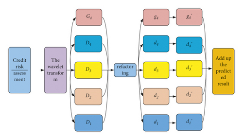
In the selection of the wavelet, Daubechies 4 with the largest applicable range was selected, and the number of decomposition layers was 4. The wavelet transform is used to decompose the price time series of the credit risk assessment. Firstly, a low-frequency approximate sequence G₄ and high-frequency detail sequences D₁, D₂, D₃, and D₄ are obtained by decomposition. The interpolation method is used to reconstruct the approximate sequence G₄ and detail sequences D₁, D₂, D₃, and D₄. LSTM was used to predict the reconstructed subsequences, and the final prediction result was obtained by summing up the predicted subsequences. The prediction process is shown in Figure 1.

Details are in the caption following the image — Open in figure viewer PowerPoint

The training parameters of the LSTM model are set as follows: the number of hidden cells of the LSTM layer is 200, the maximum number of training iterations is 200, the gradient threshold is set to 1, and the initial learning rate is 0.005. After 125 iterations, the learning rate is reduced by a multiplying factor of 0.2, and the predicted step size is 1.

2.2.2. CEEMDAN-LSTM Model

Adaptive noise-complete empirical mode decomposition (CEEMDAN) is based on an improvement of empirical mode decomposition (EMD), which is also a method for analyzing nonlinear and nonstationary data by breaking down the sequence into a series of intrinsic mode function (IMF) components to represent data features at different time scales. However, the unimproved EMD has the defect of mode aliasing, so CEEMDAN based on the white noise method of ensemble empirical mode decomposition (EEMD) proposed the improvement measure of adding independent distributed Gaussian white noise into the original data. The adaptive noise addition solved the problem of mode aliasing and excessive residual noise simultaneously and improved the decomposition efficiency. The CEEMDAN algorithm process is as follows.

(1)
We add Gaussian white noise with normal distribution on the basis of original time series as shown in the following equation:
(12)
where j(t) is the original sequence, ω^y(t) is the white Gaussian noise, ε₀ is the standard deviation of noise, and n is the number of noise addition.
(2)
The first-order modal component is obtained according to the EMD method, the mean value is taken as the first xwf component, and the residual value after the first stage is calculated as follows:
(13)
(3)
Similarly, we take the residual term as the original time series, repeat steps (1) and (2), and add the adaptive Gaussian white noise for EMD decomposition to obtain A and the corresponding residual value. We repeat the above steps until the residual can no longer be decomposed, that is, the residual term has become the xwf₂(t) monotone function or constant. When the amplitude is lower than the established threshold and cannot continue to extract the next modal function, the decomposition process ends. Finally, Z orthogonal xwf functions and the final trend term res_z are obtained as shown in the following equation:
(14)
Based on the advantages of CEEMDAN in sequence decomposition, this paper constructs the CEEMDAN-LSTM model to predict the price of the credit risk assessment.

Because the short-term fluctuation is reflected by the high-frequency component, it has little impact on the original sequence, and the average value is close to zero. Therefore, the high-frequency component can be screened through t-test, and then the new sequence can be adjusted in combination with xwf_b and other factors. The trend term reflects the trend of the original sequence. The detailed operations are as follows:

(1)
The mean value of each decomposed eigenmode xwf_x(t), x = 1,2,3, …, z was calculated.
(2)
The t-test with a 0.05 significance level and a nonzero mean for xwf_x(t) was conducted successively.
(3)
After the sequential test, the first component xwf_g(t) with a significant nonzero mean is obtained; the high-frequency subsequence xwf_b is obtained by adding xwf₁(t) to xwf_v−1(t), and the low-frequency subsequence xwf₁ is obtained by adding xwf_g(t) to xwf_z(t), res_z that continues as a trend item. Parameter settings refer to Torres parameter settings. When CEEMDAN was used to decompose the original sequence, the white Gaussian noise with a standard deviation of 0.2 was added, the number of additions was 500, and the maximum number of iterations was 2000.

2.2.3. CEEMDAN-SE-LSTM Model

Based on the above models, sample entropy is introduced as the basis for imf component reconstruction. Starting from time series complexity, the sample entropy quantitatively describes the system complexity and regularity degree so as to judge the probability of generating new patterns. The larger the calculated entropy value is, the more complex the time series is and the higher the probability of generating a new mode is. Conversely, the simpler the sequence is, the lower the probability of generating a new mode is.

The sample entropy is calculated as follows:

(1)
For given time series y(n), a set of K-dimensional vectors j_z(1), …, j_z(t − z + 1) can be obtained according to the sequence number, where j_z(x) = {j(x), j(x + 1), …, j(x + z − 1)}(1 ≤ x ≤ t − z + 1).
(2)
The distance of j_z(x) is defined as the absolute value of the maximum difference between the two corresponding elements, which are denoted as d[jz(x), jz(y)].
(3)
Given threshold h, for each I, we calculate the number of d[j_z(x), j_z(y)] < r, which is denoted as T_z(x) and defined in the following equation:
(15)
(4)
We calculate the mean of all the above defined values, which are denoted as as shown in the following equation:
(16)
(5)
We repeat the above steps to get . When n is limited, the estimated value of sample entropy SampEn is calculated as follows:
(17)
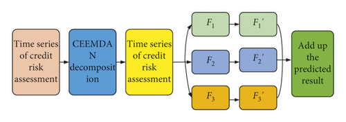
Based on the characteristics of sample entropy in judging the sequence complexity and the probability of new patterns, this paper introduces the calculation of the sample entropy as the basis of reconstruction. Different from the previous two models which take low frequency and high frequency as the basis for reconstruction, this model needs to calculate sample entropy. The closer the sample entropy, the more similar the representative components and the more consistent the fluctuations. The prediction process of this model is shown in Figure 2.

2.3. Credit Risk Assessment Model

2.3.1. Framework Design

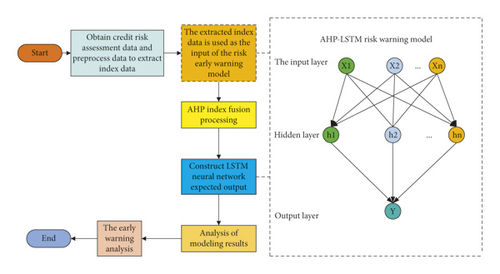
Based on the hierarchy structure of the credit risk assessment public opinion index system, we use the improved AHP combined with LSTM to establish the AHP-LSTM credit risk early warning model and to carry out the credit risk assessment network public opinion early warning analysis. The framework of the early warning model is shown in Figure 3.

The modeling process of the AHP-LSTM model proposed in this paper is as follows:

(1)
The AHP algorithm is used to analyze the training data set samples, the data feature components are obtained, and a new sample set is formed.
(2)
The LSTM network is built. We take the training set as the input of the LSTM network and samples in step 1 as the expected output of the LSTM network.
(3)
We set LSTM parameters and perform network training.
(4)
We take the test data as the input of LSTM, build a network public opinion warning model according to the expected output, and carry out the credit risk assessment and warning.

2.3.2. Model Training

Several credit risk data are selected as samples and trained by the AHP-LSTM model. Firstly, the AHP-LSTM model parameters are determined. For the adjustment of the hidden layer node number and learning efficiency, the method of control variables is adopted, and nonkey parameters are determined first. Then, the learning efficiency η was then set and attenuated at a certain speed, and the results were normalized to [0, 1.0]. In order to avoid the unsatisfactory effect of random initialization, it is necessary to conduct multiple training and finally determine the optimal parameters.

3. Result Analysis and Discussion

3.1. Data Sources and Data Preprocessing

The experiment used two data sets. 887,979 credits were issued between 2007 and 2015 and first downloaded from the LendingClub website. The specific information is listed in Table 3, in which the default samples account for 7.6% of the total samples. The data set is mainly used for experimental verification. The specific information is listed in Table 4.

3. Information description of the LendingClub data set.

The basic information	Historical loan information
Home ownership, initial rating, verification of income, number of years of service, etc	Amount of loan, amount of promised repayment, number of maturities, interest rate of loan, sum of interest so far, total amount of payment received recently, month of initiating loan, outstanding principal amount, etc

4. Information description of the PPDAI data set.

The basic information	Historical loan information
Initial rating, age, gender, mobile phone certification, household registration certification, credit investigation certification, education certification, etc	Amount of loan, term of loan, interest rate of loan, successful date of loan, type of loan, whether the first bid, number of successful loans in history, principal repaid, etc

Data preprocessing mainly includes two steps: data cleaning and feature preprocessing. The first step is to conduct data cleaning on the samples. Firstly, features with missing values greater than 95% are screened out to test whether features are closely related to default. Then, “MISSING” was used to fill in the vacancy value of categorical features from the missing value of features in the default sample. After the outliers are removed for numerical features, the corresponding feature mean value is used to fill the vacancy value. In feature preprocessing, the original features are processed to generate derivative variables. In order to reduce the computation amount, the number of category features with more categories is reduced. The data of LendingClub and PPDAI after final processing are 62 and 58 dimensions, respectively.

3.2. Parameter Debugging and Comparative Experiment

In order to ensure that the proportion of different samples in the training set and the test set is the same as that in the original data set, hierarchical sampling is used for crosscutting due to the large gap between the number of normal performance samples and default samples in the natural samples.

In the case of unbalanced positive and negative samples, the model can be predicted by the preprocessed data, and the Literature [18], Literature [19], Literature [20] and Literature [21] were selected as compared methods. The results are listed in Table 5. Due to the imbalance of positive and negative samples in the data set, the recall rate and F1 value of all methods are relatively low, but the recall rate of the AHP-LSTM model is still 15.51% higher than that of the suboptimal literature [20] method. As for the accuracy and other indicators, except the literature [19] method that has a slightly higher accuracy, the proposed method has higher accuracy than other methods. In addition, the average accuracy of this method is the highest among all methods, and the standard deviation is relatively small. Experimental results show that this method has better performance and stronger stability.

5. Performance comparison of methods in the original data set (unit: %).

Classifier	Accuracy	Precision	Recall	F₁	AUC
Literature [18]	97.51 ± 0.08	98.69	64.71	78.55	92.71
Literature [19]	97.35 ± 0.29	99.21	66.32	79.24	95.91
Literature [20]	93.31 ± 0.17	98.55	68.75	81.28	93.03
Literature [21]	97.01 ± 0.21	98.77	63.01	76.28	91.23
Proposed	98.81 ± 0.09	99.41	84.26	92.18	98.16

In addition, in order to balance positive and negative samples, the undersampling operation is performed on the preprocessed data. The experimental results are listed in Table 6. All indexes of the AHP-LSTM model are higher than those of other methods except that the literature [21] model has a slightly higher accuracy. The average accuracy of this method is the highest among all methods, and the standard deviation is relatively small. The above two experiments show that the AHP-LSTM model still has strong stability in the case of unbalanced positive and negative samples.

6. Performance comparison of methods in the undersampled data set (unit: %).

Classifier	Accuracy	Precision	Recall	F₁	AUC
Literature [18]	86.21 ± 0.09	94.49	71.98	80.21	93.19
Literature [19]	91.81 ± 0.17	98.27	84.32	90.66	96.46
Literature [20]	82.44 ± 0.15	81.13	78.85	79.98	90.66
Literature [21]	92.09 ± 0.77	97.58	83.77	90.29	96.61
Proposed	96.18 ± 0.12	97.21	94.63	95.09	99.36

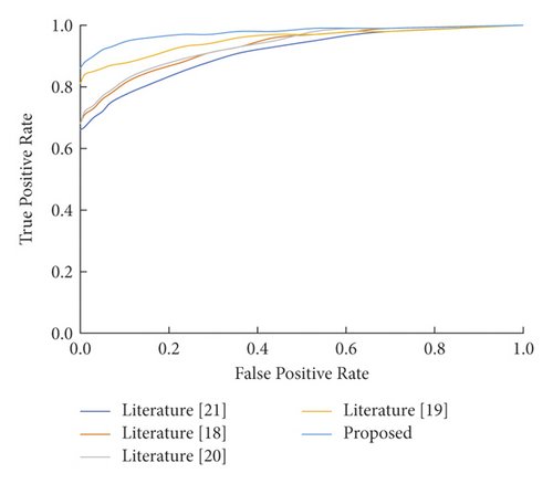
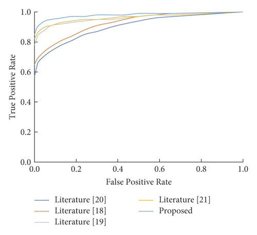
In the LendingClub data set, ROC curves of different methods before and after undersampling of normal performance samples are shown in Figures 4 and 5. The closer the curve is to the upper left corner (0,1) in the ROC curve, the better the performance. As can be seen from Figures 4 and 5, under the same FPR, the TPR of the AHP-LSTM model method is higher than that of other compared methods, indicating that the AHP-LSTM model method has better performance.

To verify the stability and universality of the method in this paper, the model is used to evaluate the credit risk of borrowers in the PP DAI data set. The experimental results of each method are listed in Table 7. The indexes of the AHP-LSTM model method and compared method are mostly more than 95%, especially the accuracy and the other indexes of the AHP-LSTM model method reach 100%, which is higher than other compared methods, due to the small gap between experimental results under different methods.

7. Performance comparison of methods in the PPDAI data set (unit: %).

Classifier	Accuracy	Precision	Recall	F₁	AUC
Literature [18]	99.22 ± 0.07	99.91	91.59	95.67	99.97
Literature [19]	99.85 ± 0.08	100	99.79	99.85	99.99
Literature [20]	99.78 ± 0.15	99.83	97.54	98.61	99.98
Literature [21]	99.31 ± 0.13	99.39	91.69	95.53	99.81
Proposed	99.98 ± 0.04	100	100	99.99	100

3.3. Display and Analysis of the Feature Importance Score

Based on the LendingClub data set, this paper constructs the CREDIT risk assessment model of P2P online loan borrowers based on the AHP-LSTM model and solves the feature importance score of the model so as to explain the model to some extent. The top ten features of feature importance are selected here, and their normalized importance values are listed in Table 8. Among them, the first “initial rating” refers to the user credit rating assessed by the letter of credit, which is divided into three levels: A, B, and C. Each level is divided into 1, 2, and 3 categories. Among them, A1 borrowers have the best credit rating and different credit ratings reflect the credit quality of borrowers. “Certified status” indicates whether LendingClub has verified the borrower’s income. The verified income indicates that the borrower’s income is real and relatively reliable. The “home state” refers to the state where the borrower lives when applying for a loan. In dealing with this feature, this paper divides the 50 states of the United States into three categories according to their economic development level. States with high economic development levels have many borrowers and a large number of defaults. The purpose of the loan is mainly divided into debt consolidation, credit card repayment, house decoration, and other situations, and people with different borrowing purposes have different default rates. Finally, as for the loan interest rate, the number of repayments due this month and other characteristics, the higher the loan interest rate and amount, and the greater the borrower’s probability of default are taken into account.

8. Feature importance scores in the LendingClub data set.

The serial number	Characteristics	Normalized value of importance
1	Initial rating	0.1698
2	Certification status	0.0621
3	State	0.0538
4	Borrowing purposes	0.0391
5	Borrowing rates	0.0283
6	The amount due this month	0.0271
7	The total amount of all loans should be repaid	0.0262
8	The total amount of the loan should be repaid	0.0262
9	The total amount of interest received to date	0.0256
10	The total amount pledged by the lender	0.0253

Similarly, in the PPDAI data set, this paper uses the credit model based on the AHP-LSTM model to predict. The normalized values of the top 10 features and importance in the feature importance score are listed in Table 9. In both data sets, the “initial rating” takes the first place, so it can be used as an important reference index for the lender to predict whether the borrower defaults. The“loan type” can be divided into safety standard receivables, e-commerce, the ordinary standard, etc. The ordinary standard is the most common type of standard. Security standard receivable refers to the standard that the lender meets the amount of safety standard receivables that is greater than a certain value, and the loan credit score is greater than a certain value. E-commerce means that the borrower has passed the e-commerce certification, and the store runs well. It can be seen that the division of different populations has a certain influence on the prediction results of the model. In addition, mobile phones, household registrations, and other certifications reflect the authenticity of information filled in by borrowers, which is of certain importance to model prediction.

9. Feature importance scores in the PPDAI data set.

The serial number	Characteristics	Normalized value of importance
1	Initial rating	0.2141
2	Borrowing type	0.1532
3	Whether the header	0.0439
4	The phone authentication	0.0421
5	Last repayment date	0.0428
6	Gender	0.0409
7	Registered permanent residence certificate	0.0318
8	Degree certificate	0.0307
9	Borrowing amount	0.0291
10	Taobao certification	0.0275

To sum up, the model can screen out features that greatly impact the prediction of whether a borrower defaults and the importance score of features conforms to people’s objective and intuitive understanding.

4. Conclusion

With the continuous development of the financial industry, consumer financial risks greatly impact the market and individuals. The accuracy of personal credit risk assessment plays a positive role in reducing the losses of banks, consumer finance, and other lending institutions, which is conducive to the stability of the market. Based on the analytic hierarchy Process (AHP) and the LSTM model, this paper evaluates individual credit risk through the improved AHP and the optimized AHP-LSTM model. Based on the LendingClub and PPDAI data sets, the experiment uses the AHP-LSTM model method to classify and predict. It is compared with the random forest and the wide and deep model. Experimental results show that the performance of this method is superior to other comparison methods in both data sets, especially in the case of unbalanced data sets. In addition, this paper explains the prediction results of the model through the measure of feature importance, which is in line with people’s intuitive and objective understanding. In order to solve the problem of sample class imbalance, this paper simply uses undersampling technology to balance the model. In the follow-up work, cost-sensitive learning or other more effective class imbalance learning methods can be combined to improve the model performance further. In addition, to enhance the practicability and stability of the model, it can be applied more fully to the anticheating scenario. However, when the dimension of data features is high and sparse, the algorithm in this paper may not be able to find the optimal subspace, which is also the direction of further optimization.

Conflicts of Interest

The authors declare that there are no conflicts of interest.

Acknowledgments

This work was supported by the Shijia Zhuang University of Applied Technology.

Open Research

Data Availability

The labeled data set used to support the findings of this study is available from the corresponding author upon request.

References

1 Ramsay I. and Williams T., Peering forward, 10 Years after: international policy and consumer credit regulation, Journal of Consumer Policy. (2020) 43, no. 1, 209–226, https://doi.org/10.1007/s10603-019-09436-x.
10.1007/s10603-019-09436-x
Web of Science® Google Scholar
2 Li Y., Gao W., and Ruan Y., Performance investigation of grid-connected residential PV-battery system focusing on enhancing self-consumption and peak shaving in Kyushu, Japan, Renewable Energy. (2018) 127, 514–523, https://doi.org/10.1016/j.renene.2018.04.074, 2-s2.0-85051681132.
10.1016/j.renene.2018.04.074
Web of Science® Google Scholar
3 Blackwell T. and Kohl S., The origins of national housing finance systems: a comparative investigation into historical variations in mortgage finance regimes, Review of International Political Economy. (2018) 25, no. 1, 49–74, https://doi.org/10.1080/09692290.2017.1403358, 2-s2.0-85038031805.
10.1080/09692290.2017.1403358
Web of Science® Google Scholar
4 Bhatore S., Mohan L., and Reddy Y. R., Machine learning techniques for credit risk evaluation: a systematic literature review, Journal of Banking and Financial Technology. (2020) 4, no. 1, 111–138, https://doi.org/10.1007/s42786-020-00020-3.
10.1007/s42786-020-00020-3
Google Scholar
5 Soekapdjo S., Nugroho L., Badawi A., and Utami W., Bad debt issues in Islamic bank: macro and micro influencing (Indonesia cases), International Journal of Commerce and Finance. (2018) 4, no. 1, 10–26.
Google Scholar
6 Wang F. M., Wang L. M., Wang T., Lya Z. Y., and Cui L. H., MRI image denoising based on an improved threshold, Journal of Beijing University of Chemical Technology (Natural Science Edition). (2022) 49, no. 1, 122–127.
Google Scholar
7 Rahman A., Chowdhury M E H., Khandakar A., Kiranyaz S., Zaman K. S., Reaz M B I., Islam M T., Ezeddin M., and Kadir M A., Multimodal EEG and keystroke dynamics based biometric system using machine learning algorithms, IEEE Access. (2021) 9, 94643, https://doi.org/10.1109/access.2021.3092840.
10.1109/ACCESS.2021.3092840
Web of Science® Google Scholar
8 Ali H., Salleh M. N. M., Saedudin R., and Kashif H., Imbalance class problems in data mining: a review, Indonesian Journal of Electrical Engineering and Computer Science. (2019) 14, no. 3, 1560–1571, https://doi.org/10.11591/ijeecs.v14.i3.pp1552-1563, 2-s2.0-85065230621.
10.11591/ijeecs.v14.i3.pp1552-1563
Google Scholar
9 Papouskova M. and Hajek P., Two-stage consumer credit risk modelling using heterogeneous ensemble learning, Decision Support Systems. (2019) 118, 33–45, https://doi.org/10.1016/j.dss.2019.01.002, 2-s2.0-85059804281.
10.1016/j.dss.2019.01.002
Web of Science® Google Scholar
10 Jones S. and Wang T., Predicting private company failure: a multi-class analysis, Journal of International Financial Markets, Institutions and Money. (2019) 61, 161–188, https://doi.org/10.1016/j.intfin.2019.03.004, 2-s2.0-85063758554.
10.1016/j.intfin.2019.03.004
Web of Science® Google Scholar
11 Abdolrasol M, Hussain S., Ustun T S., Sarker M., Hannan M A., Mohamed R., Ali J., Mekhilef S., and Milad A., Artificial neural networks based optimization techniques: a review, Electronics. (2021) 10, no. 21, https://doi.org/10.3390/electronics10212689.
10.3390/electronics10212689
Web of Science® Google Scholar
12 Qin H., Fan P., Tang H., Huang P., Fang B., and Pan S., An effective hybrid discrete grey wolf optimizer for the casting production scheduling problem with multi-objective and multi-constraint, Computers & Industrial Engineering. (2019) 128, 458–476, https://doi.org/10.1016/j.cie.2018.12.061, 2-s2.0-85059257086.
10.1016/j.cie.2018.12.061
Web of Science® Google Scholar
13 Murthy N. S. and Bethala C., Review paper on research direction towards cancer prediction and prognosis using machine learning and deep learning models, Journal of Ambient Intelligence and Humanized Computing. (2021) 12, 1–19.
PubMed Google Scholar
14 Syukron M., Santoso R., and Widiharih T., Perbandingan metode smote random forest dan smote xgboost untuk klasifikasi tingkat penyakit hepatitis C pada imbalance class data, Jurnal Gaussian. (2020) 9, no. 3, 227–236, https://doi.org/10.14710/j.gauss.v9i3.28915.
10.14710/j.gauss.v9i3.28915
Google Scholar
15 Maldonado S. and López J., Dealing with high-dimensional class-imbalanced datasets: e, Applied Soft Computing. (2018) 67, 94–105, https://doi.org/10.1016/j.asoc.2018.02.051, 2-s2.0-85043459317.
10.1016/j.asoc.2018.02.051
Web of Science® Google Scholar
16 Li Z., Tian Y., Li K., Zhou F., and Yang W., Reject inference in credit scoring using semi-supervised support vector machines, Expert Systems with Applications. (2017) 74, 105–114, https://doi.org/10.1016/j.eswa.2017.01.011, 2-s2.0-85009461275.
10.1016/j.eswa.2017.01.011
Web of Science® Google Scholar
17 Havrylchyk O. and Verdier M., The financial intermediation role of the P2P lending platforms, Comparative Economic Studies. (2018) 60, no. 1, 115–130, https://doi.org/10.1057/s41294-017-0045-1, 2-s2.0-85040033238.
10.1057/s41294-017-0045-1
Web of Science® Google Scholar
18 Christodoulou E., Ma J., Collins G S., Steyerberg E W., and Verbakel Y J., A systematic review shows no performance benefit of machine learning over logistic regression for clinical prediction models, Journal of Clinical Epidemiology. (2019) 110, 12–22, https://doi.org/10.1016/j.jclinepi.2019.02.004, 2-s2.0-85062005742.
10.1016/j.jclinepi.2019.02.004
PubMed Web of Science® Google Scholar
19 Denisko D. and Hoffman M. M., Classification and interaction in random forests, Proceedings of the National Academy of Sciences. (2018) 115, no. 8, 1690–1692, https://doi.org/10.1073/pnas.1800256115, 2-s2.0-85042191230.
10.1073/pnas.1800256115
CAS PubMed Web of Science® Google Scholar
20 Cervantes J., Garcia-Lamont F., Rodríguez-Mazahua L., and Lopez A, A comprehensive survey on support vector machine classification: a, Neurocomputing. (2020) 408, 189–215, https://doi.org/10.1016/j.neucom.2019.10.118.
10.1016/j.neucom.2019.10.118
Web of Science® Google Scholar
21 Cao Y. and Gu Q., Generalization bounds of stochastic gradient descent for wide and deep neural networks, Advances in Neural Information Processing Systems. (2019) https://doi.org/10.48550/ARXIV.1905.13210.
10.48550/ARXIV.1905.13210
PubMed Google Scholar

Citing Literature

All articles

Improved AHP Model and Neural Network for Consumer Finance Credit Risk Assessment

Abstract

1. Introduction