[Retracted] Modeling and Analysis of Multifocus Picture Division Algorithm Based on Deep Learning
Abstract
As a complex machine learning algorithm, deep learning can extract object shape information and more complex and advanced information in images by using a deep learning model. In order to solve some problems of deep learning in image feature extraction and classification, this paper designs a modeling method of multifocus image segmentation algorithm based on deep learning. The acceleration effect of FPGA (field programmable gate array) on deep learning and weight sharing is analyzed. By introducing deep learning, the trouble of determining the weight coefficient is eliminated, and the energy function is simplified. Therefore, the relevant parameters of multifocus image segmentation can be easily set, and better results can be obtained. The multifocus image segmentation algorithm based on deep learning can not only obtain closed and smooth segmentation curves but also adaptively deal with topology changes due to high segmentation accuracy and stable algorithm. The results show that the model effectively combines the local and global information of the image, so that the model has good robustness. The depth learning algorithm is used to calculate the average value of local inner and outer pixels of an image. Even for complex images, relatively simple contour curves can be obtained.
1. Introduction
Images are able to describe what people see with their eyes; however, it is quite difficult for computers to process human visual objects [1]. The multifocus picture division is a key step from picture handling to analysis of pictures, which is aimed at dividing the image into several specific regions with unique properties and extract the target of interest [2]. The advent of computers has provided the possibility to study images in greater depth and with the help of computer technology, image engineering has gradually evolved. Deep learning is a large-scale nonlinear circuit with real-time signal processing capability; like cellular automata, it consists of a large number of cellular elements and allows direct communication between only the closest cells [3]. Multifocus image segmentation is a crucial step from image processing to image analysis and is a fundamental computer vision technique [4]. In image analysis, entropy, as a statistical feature of an image, captures the magnitude of the quantity of data contained in the image [5]. This is due to the fact that image segmentation, separation of objectives, extraction of characteristics, and determination of parameters transform the raw picture into a more extracted and compressed shape, which makes higher layer of analysis and comprehension feasible [6].
A multifocus picture division is a difficult and hot point in picture handling, which makes the basic pavement for the analysis and reconstruction of the image later [7]. The picture handling system can be expressed in three levels, and the combination of these three levels is also called image engineering low-level processing techniques which mainly include image filtering, image enhancement, image restoration, image restoration, and image coding and compression. The multifocused picture division is a class of picture handling between the bottom-level picture handling and the middle-level analysis of pictures. Picture division is an important element in analysis of pictures, which is the process of dividing the original image into several subregions that are not connected to each other and extracting the part of interest from these regions [8]. Traditional picture division methods are mainly based on the underlying image features that can be observed by the human eye, such as color, texture, and edges [9]. When there is a large difference between the target and the background in the image, it can be segmented completely. However, when the features such as grayscale and color of the target and the background are closer or the background in the image is complex, the segmentation results obtained by traditional picture division methods often have more missplitting and the segmented targets are incomplete and lack of detail information [10].
CNN (convolutional neural network) is a locally connected network in which each unit is interconnected only with its neighboring neurons, and the influence of other neurons in the neighborhood is realized by passing information from unit to unit. Simply put, it is a machine learning algorithm that gives computers the ability to learn potential patterns and features from a large amount of existing data to be used for intelligent recognition of new samples or to anticipate the likelihood of something in the future. The advantage is that its multilayer structure can automatically extract different levels of distinguishing features of an image from a large number of samples, and these features are more effective and robust compared to the underlying features designed and extracted manually. The multifocus picture division is the key process from analysis of pictures to image understanding, separating the region of interest from the image, which simplifies the complexity of picture handling on the one hand and provides the basis for subsequent extraction of image features and quantitative analysis on the other.
- (1)
In order to assist the complete segmentation of the region, the representation of the target shape is particularly important. In this paper, the shape is characterized by building a model, and subsequently, the a priori shape information is used to assist the multifocus picture division
- (2)
With the introduction of deep learning, the trouble of determining the weighting coefficients is eliminated and the energy function is simplified; thus, it is easy to set the relevant parameters for the multifocus picture division and obtain better results
- (3)
The multifocus picture division algorithm based on deep learning can not only obtain closed and smooth segmentation curves but also handle topological changes adaptively due to the high segmentation accuracy and stable algorithm
2. Modeling Idea of Multifocus Picture Division Algorithm Based on Deep Learning
2.1. Construction Method of Conditional Random Field Model
The conditional random field is a discriminative model for modeling the probability distribution between the marker X and the observation Y. In the multifocus picture division, if the kind of similarity present in the same region is particularly valued and the uniformity of the segmented region is required too much, it will result in many blank regions or irregular edges. If there is a difference in the gray value between the target and the background in a gray image, the target and the background in the image can be separated by threshold segmentation. If only one threshold is selected, the segmentation is called single-threshold segmentation, which will divide the image into two parts: the target and the background. The segmentation with multiple thresholds is called multithreshold segmentation, which will divide the graph into multiple regions.
where Jp(t) is the p group input objective function.
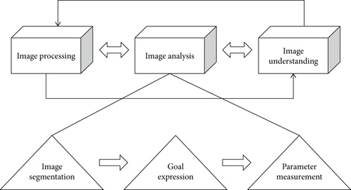
The conditional random field model can combine knowledge and experience of the target to be segmented based on the underlying visual properties of the image itself such as edge, texture, grayscale, and color, and the target to be segmented, such as the shape, brightness, color, and other empirical knowledge of the target, in an organic way. Depending on the level of abstraction and the research method, there are three characteristic levels: picture handling, analysis of pictures, and image understanding. This is shown in Figure 1 below.
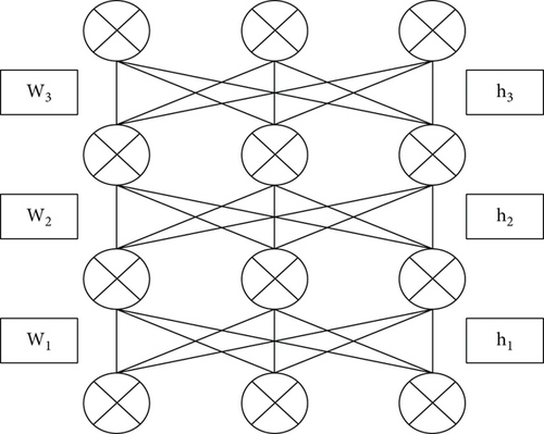
First, the conditional probability is defined using the DBN network and the marker variables of pixel points on the graph structure and the marker variables of neighboring pixel points. The basic unit of DBN is the cell: it contains linear and nonlinear circuit elements, typical elements are linear capacitance, linear resistance, and linear and nonlinear controlled and independent current sources. The structure of DBN is no connection within the top two layers, full connection between each layer, and the remaining other layers are The DBN model structure is shown in Figure 2.
where rij is the correlation coefficient of the ith evaluation sample with the jth indicator.
where T is the unprocessed input value, Tmax is the maximum value of neural network input, and Tmin is the minimum value of neural network input.
Since SFM can accept input images of arbitrary size, the feature map of the last convolutional layer is upsampled using a deconvolution layer to restore it to the same size as the input image. Thus, a prediction can be generated for each pixel while preserving the spatial information in the original input image. After the division of pixel points is completed, the two types of pixel points form two image regions representing the target and the background, respectively, and the segmentation is completed.
Finally, the identification of the markers in the image is done by two potential functions and the characteristic observed data of the whole image. The best marker Y, which is the marker corresponding to the maximum a posteriori probability, can be converted into the minimization of the energy function. Therefore, it is most convenient to use threshold segmentation when the difference between target and background grayscale in the original image is more obvious. Threshold segmentation accomplishes the work of obtaining a closed contour of a given shape from the (discontinuous) edge points in the image space by an accumulation operation in the parameter space. When using the region extraction method, the pixels are assigned to individual objects or regions; in the boundary method, only the boundary between the presence and the region needs to be determined; in the edge method, the edge pixels are first determined and they are connected to form the desired boundary. Meanwhile, the high resolution of downsampling is fused with the features of upsampling to further improve the accuracy of segmentation localization. Most importantly, deep learning can be loaded on smart mobile terminals, which in turn makes it easier and faster to receive data from remote servers and upload and download the data.
2.2. Model Structure of Multifocus Picture Division Algorithm
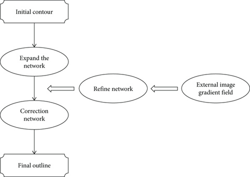
The multifocus picture division algorithm model uses the SegNet model as the backbone network for segmentation, which contains two components: an encoder and a decoder. The multifocus picture division algorithm is done by the DTCNN that finds the image gradients one at a time and is invariant throughout the multilayer iterations. The processing module for each direction is composed of 3 DTCNN networks: the contour curve expansion network, the refinement network, and the correction network, as shown in Figure 3.
where is the convolution window of the i word which is the characteristic representation of k.
The cloud computing layer uploads the scene images and performs multifocus picture division using the FCN8-VGG16 network when the network is open. The trained U-Net model is downloaded, and the segmented image and U-Net model at the remote cloud server are uploaded to the smart mobile terminal via a 5G mobile network. The mechanism that drives the contour motion lies in minimizing the energy function when making the region that satisfies the consistency expand to the maximum or contract to the minimum, i.e., the boundary of the consistency region.
where ωij is the weight of hidden layer and output.
where ‖xp − ci‖ is the norm of xp − ci, xp is the sample data input by the input layer, and ci and σ re the center and width of radial basis function.
The principle is to design the fitting target with a set of curves to be selected and define the energy function associated with each curve in the set to be selected. The energy function is designed with the principle that favorable properties lead to energy reduction, including continuity and smoothness of the curves. The remote service component layer serves remote procedure calls through a web server in the background and tensor flow on the GPU (graphics processing unit) to perform image transfer and data processing operations. Therefore, the model can be used to process large image databases, and the picture division model in this paper is highly efficient and robust compared to the commonly used picture division models.
3. Application Analysis of Deep Learning in Multifocus Picture Division Algorithm Modeling
3.1. FPGA Accelerated Analysis of Deep Learning
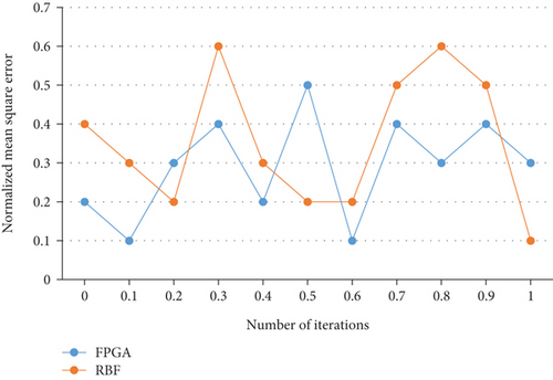
This section explores FPGA (field programmable gate array) acceleration schemes for deep learning to enable fast and efficient processing of data for deep learning. For those images with strong contrast between target and background, the method can quickly and accurately segment multi-focused images into the images we want. The value of FPGA acceleration is that it provides a unified solution to a range of computer vision problems and has been successfully applied to computer vision fields such as boundary extraction, picture division and classification, motion tracking, 3D reconstruction, and stereo visual matching. The mean square error of deep learning after FPGA acceleration is also consistently lower than that of RBF neural network, indicating that FPGA acceleration can improve the prediction accuracy of the model, and the model mean square error comparison is shown in Figure 4 below.
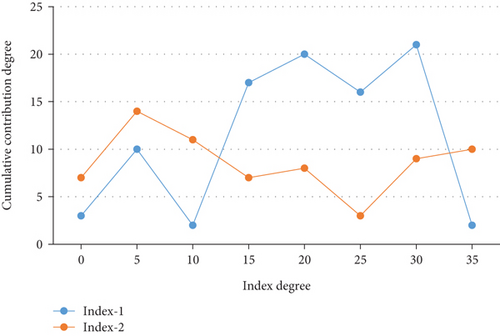
First, the process of computing the product accumulation of the input feature map and the weight matrix needs to be performed K∗K∗N times the product accumulation of the weights and the input, and the N input feature map is convolved to obtain the M size R∗C output feature map. In order to obtain the color feature probability distribution of target and background, the initial region information of manual marker needs to be extracted separately. The convolutional characteristics of the appropriate phase in the encoder and decoder are coupled in a cascade by channel splicing and then fed into a newly convolutional level to be further learned and complete the ultimate classification forecast. The proposed deep learning is used to analyze the multifocus picture division evaluation metrics, and the metrics that contribute the most to the picture division are filtered out, and the results of the principal component analysis are shown in Figure 5 below.
When the value of this pixel is +1, if the sum of the pixel values in its neighborhood is greater than the threshold, then this pixel is not an edge pixel and the value of this pixel tends to 0. Conversely, if the sum of the pixel values in its neighborhood is less than this threshold, then this pixel is an edge pixel. As for the position of the boundary, since the serial approach takes fuller consideration and relies on the previously obtained results when making the current decision, the accuracy of the position of the whole boundary is easily guaranteed to be high if the starting point is chosen correctly.
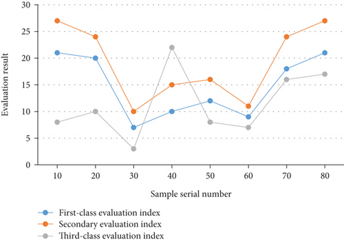
Secondly, when two matrices are matrix multiplied, each output result needs to take one row and one column of data of the two matrices, respectively, for product accumulation to get the final result. The manually extracted target and background pixels both have the same pattern information, so the color feature space can be described by pattern points. Prior to coupling the cascade of convolutional characteristics in each of the latter three phases in the encoder and decoder, the sophistication of the model after cascading multiple levels of features can be reduced to simplify the training of the model, and the level dependence of the characteristics extracted from the deeper convolutional layers is considered to maintain the local consistency of the features and improve the performance of division. Boundary tracking finds the neighboring points with the highest gray level from the original image and finds the neighboring points with the maximum gray level as the boundary points. In the specific implementation, it is necessary to first find a raw pixels for each image zone to be divided as the growing starting position, then take the raw pixels and compare them with the pixels in the surrounding neighborhood, and if there are pixels with the identical or comparable properties to the raw pixels, they are incorporated into the zone where the raw pixels are situated. The neural network is able to automatically learn previous experience from the provided data samples without the tedious process of searching and representation and is able to automatically approximate those functions that best portray the laws of the sample data, and the evaluation results under different sample order numbers are shown in Figure 6.
Finally, to reduce the number of repeated accesses from off-chip memory DDR, on-chip storage is used to cache the input data and the weight matrix. The initial marker region is smoothed and filtered using the same pattern points that many pixels have to characterize the local feature points corresponding to some pixels. The use of pattern points to describe the color feature space allows for a significant reduction in algorithm complexity when estimating whether a pixel belongs to the target or the background. Since pixels in the same region of the original image have similar features, these pixels are combined to form different regions by some predefined rules (growth rules). Thus, in a noise-free monotonic point-like image, this algorithm will trace the maximum gradient boundary, but even a small amount of noise will make the tracking temporarily or permanently off-boundary. For feature fusion, the CMLFDNN model amplifies the last three phases of features in the encoder and decoder, respectively, level-by-level and does pixel-by-pixel summation to fuse them prior to coupling them in cascade, which takes into account the dependency of the levels of accumulated characteristics retrieved in different convolution phases and maintains the local consistency of the active contours. In this way, the active contour can converge to the local boundary under the guidance of the energy function as it moves within the range of values taken, and the continuity and smoothness of the curve itself are maintained.
3.2. Weight Sharing Analysis of Deep Learning
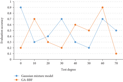
In the case of the same spectral difference, if the spatial distance or image gradient is smaller, the weight is larger; on the contrary, the weight is smaller. For example, the neighboring pairs of points on both sides of the potential boundary have a small distance but a large gradient. The traditional weight sharing model is generally based on the Gaussian mixture model, which is also very simple and effective in multifocus picture division algorithms. The Gaussian mixture model is a kind of highly global optimization-seeking model, which is widely used in the fields of signal processing, image processing, and pattern recognition. The accuracy curve of the model evaluation is shown in Figure 7.
However, there is noise in segmentation and there are many segmentation algorithms based on a small number of local data points. Therefore, weight sharing based on deep learning has the interactive ability to represent the shape of anatomical structures concisely and analytically and segment the target boundary precisely. In deep learning, each convolution filter of the convolution layer is repeatedly applied to the whole perceptual field to convolve the input image, and the convolution result constitutes the feature map of the input image to extract the local features of the image.
First of all, in deep learning, it is assumed that layer m − 1 is the input layer and all neuron nodes in layer m are connected with all neuron nodes in layer m − 1. The process of convolutional computation to matrix multiplication is actually merging the input loop and the convolutional kernel loop, and merging the output row loop, thus reducing the number of loops to 2. In other words, take a point first and then compare the adjacent points. If they are similar, they will be merged together. If they are not similar, the calculation will be stopped immediately. Then, the gradient of the energy generalization function is calculated and the evolution equation of the level set function is obtained by using the continuous gradient descent method, and the final zero level set is determined as the multifocus picture division result. Here, it is assumed that the subsampling layer in the network is in the middle of the two convolutional layers, and if the postlevel sampling layer is a fully connected layer, we can solve the sensitivity map for subsampling directly. That is, an unsupervised codec network is trained to extract the deep features of the input image, and then, these features and spatial frequencies are used to measure the image pixel activity and obtain the decision map. Under the condition of limited training sample data, increasing the number of convolutional filters in the network model will make the number of weight parameters to be learned increase, which may cause the network to be difficult to reach a steady state during the training process. The experimental results of the four network models are compared as shown in Table 1 below.
| Classifier | C1 | C2 | C3 | Misclassification rate |
|---|---|---|---|---|
| Conv-net-1 | 3 | 17 | 26 | 8% |
| Conv-net-2 | 4 | 24 | 32 | 17% |
| Conv-net-3 | 7 | 27 | 41 | 27% |
Second, the m layer feature image contains neurons, and the weight parameters are shared among different connections, so we can still use gradient descent to learn the shared weight parameters. The equivalent mapping of convolution calculation into matrix multiplication simplifies the loop structure, which is more suitable for FPGA design and more convenient for subsequent design optimization. In the reverse update phase of deep learning, the cost function will change very slowly at first, and then, the learning process of the network will become very slow. Therefore, the strength of the final gradient at each location will be enhanced by the nearby gradients by weighting the gradient at each location in the local window. That is, the loss function is constructed based on the deviation of the output result from the desired result, and the weights of the ω are continuously adjusted using the BP algorithm to minimize the result of the loss function. Since both edges and noise are grayscale discontinuities, it is difficult to overcome the effect of noise by directly using differential operations. Therefore, the image should be smoothed and filtered before detecting the edges with the differential operator and then apply the consistency check method to adjust the decision map to get the final decision map. The performance of the deep learning-based multifocus picture division algorithm model in this paper is compared with the GA-BPNN evaluation model and SVM-based evaluation model. The simulation data remain unchanged, showing that the constructed genetic algorithm optimized RBF neural network model has high evaluation accuracy and computational efficiency, as shown in Figure 8 below.
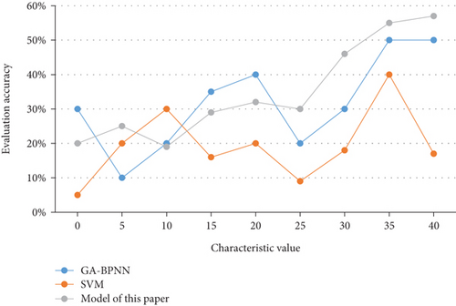
Finally, an improvement to the original gradient descent method is needed to make the gradient of the shared weights the sum of the gradients of the shared connection parameters without considering the location of the local features when feature extraction is performed on the image. In the process of converting the convolution calculation into matrix multiplication, the input feature map does not need to be changed, but the size of the weight matrix and the order of data arrangement need to be rearranged. Considering the resource limitation of the FPGA, N = 5 is set, in which case the resource consumption of the three LSTM models is shown in Table 2.
| Available | 256-node language model | 428-node language model | 639-node language model | |
|---|---|---|---|---|
| ALMs | 23189 | 65% | 49% | 37% |
| RAMs | 18924 | 38% | 28% | 19% |
| DSPs | 9956 | 42% | 39% | 26% |
The cost function is redefined and the partial derivatives of the cost function with respect to the weights and biases are positively correlated with the errors. When the error is large, the bias derivatives are guaranteed to be relatively large even if the derivative values of the nodes are small at this time, thus making the learning rate relatively large. This makes it suitable for detecting changes in focus and has the best overall detection performance under normal imaging conditions. The image can be divided into regions, and the convolution kernel of the first network layer calculates these regions separately. After the convolution kernel gets the feature responses for these regions, the responses are used as input data for the second network layer, and so on. Training deep learning through supervised learning enables the network to learn the complementary relationships of different focused regions in the original image to achieve a globally clear image.
4. Conclusions
Image target segmentation refers to the assignment of a category label to each pixel in an image. It plays a forward and backward role in the whole study, both as a test of the effectiveness of all image preprocessing and as a basis for subsequent analysis of pictures and interpretation. However, for the variational level set model where the internal energy is a length generalized function, the conventional picture division calculating the Sobolev gradient of the whole energy generalized function does not show higher computational efficiency. And deep learning algorithms are widely used for processing various types of data such as images, videos, sounds, and texts. It is capable of various tasks such as image recognition, target detection, speech recognition, and machine translation and has achieved great success in various fields such as security, medical, entertainment, and finance. A convolutional neural network is a classical deep learning algorithm that combines feature extraction and classification problems, omitting the work of manual rule-based feature extraction. In this paper, we design a modeling method for the multifocus picture division algorithm based on deep learning and analyze FPGA acceleration for deep learning and weight sharing. The model effectively combines the local and global information of the image, which makes the model have better robustness. The method of deep learning computation is used in calculating the local internal and external pixel averages of the image, and a relatively simple contour curve can be obtained even for complex images.
Conflicts of Interest
The author declares that he/she has no known competing financial interests or personal relationships that could have appeared to influence the work reported in this paper.
Open Research
Data Availability
The data used to support the findings of this study are available from the corresponding author upon request.


