Volume 2022, Issue 1 8063888

Review Article

Open Access

Pell Collocation Method for Solving the Nonlinear Time–Fractional Partial Integro–Differential Equation with a Weakly Singular Kernel

M. Taghipour

orcid.org/0000-0001-6289-6808

Department of Applied Mathematics and Computer Science, Faculty of Mathematical Sciences, University of Guilan, P.O. Box 1914, Rasht 41938, Iran guilan.ac.ir

Search for more papers by this author

H. Aminikhah,

Corresponding Author

H. Aminikhah

[email protected]

orcid.org/0000-0002-2378-5782

Department of Applied Mathematics and Computer Science, Faculty of Mathematical Sciences, University of Guilan, P.O. Box 1914, Rasht 41938, Iran guilan.ac.ir

Center of Excellence for Mathematical Modelling, Optimization and Combinational Computing (MMOCC), University of Guilan, P.O. Box 1914, Rasht 41938, Iran guilan.ac.ir

Search for more papers by this author

M. Taghipour,

M. Taghipour

orcid.org/0000-0001-6289-6808

Department of Applied Mathematics and Computer Science, Faculty of Mathematical Sciences, University of Guilan, P.O. Box 1914, Rasht 41938, Iran guilan.ac.ir

Search for more papers by this author

H. Aminikhah,

Corresponding Author

H. Aminikhah

[email protected]

orcid.org/0000-0002-2378-5782

Department of Applied Mathematics and Computer Science, Faculty of Mathematical Sciences, University of Guilan, P.O. Box 1914, Rasht 41938, Iran guilan.ac.ir

Center of Excellence for Mathematical Modelling, Optimization and Combinational Computing (MMOCC), University of Guilan, P.O. Box 1914, Rasht 41938, Iran guilan.ac.ir

Search for more papers by this author

First published: 23 May 2022

https://doi.org/10.1155/2022/8063888

Citations: 2

Academic Editor: Youssri Hassan Youssri

Share a link

Email
Wechat
Bluesky

Abstract

This article focuses on finding the numerical solution of the nonlinear time–fractional partial integro–differential equation. For this purpose, we use the operational matrices based on Pell polynomials to approximate fractional Caputo derivative, nonlinear, and integro–differential terms; and by collocation points, we transform the problem to a system of nonlinear equations. This nonlinear system can be solved by the fsolve command in Matlab. The method’s stability and convergence have been studied. Also included are five numerical examples to demonstrate the veracity of the suggested strategy.

1. Introduction

Nowadays, fractional partial differential equations (FPDEs) have emerged as one of the most crucial issues due to their vast applications in various branches of science, such as medicine [1, 2], control theory [3–5], engineering [6, 7], viscoelasticity [8], mathematical physics [9], geo–hydrology [10], signals [11], stochastic models [12], electrical engineering, [13], and financial economics [14]. Due to the fact that analytical solutions of FPDEs are rarely available, the use of numerical methods is inevitable. Hitherto, a number of numerical methods for FPDEs have been suggested, such as finite difference [15, 16], spectral methods [17–21], homotopy methods [22, 23], and finite element [24, 25]. The nonlinear FPDEs have been extensively analyzed using numerical methods. Dehghan et al. used the homotopy analysis method to construct a scheme for solving the fractional KdV equation [26]. Nikan et al. proposed a meshless technique in order to solve the nonlinear fractional fourth–order diffusion equation [27]. Safari and Azarsa introduced a meshless method based on Muntz polynomials to solve nonlinear and linear space fractional partial differential equations [28]. Yaslan applied the Legender collocation method for solving nonlinear fractional partial differential equations [29].

When it comes to solving differential equations, spectral approaches are extremely effective. The solution to the differential equation is sought as a series of basis polynomials using this method. The Galerkin, Tao, and collocation approximations are the most common spectral methods [30, 31]. For example, Samiee et al. [20] designed a Petrov–Galerkin spectral method for distributed–order PDEs. Agarwal et al. [32] suggested a spectral collocation approach for variable–order fractional integro–differential equations. In [33], the authors used the polynomial–sinc collocation method for solving distributed order fractional differential equations. Abbaszadeh et al. proposed a Crank–Nicolson Galerkin spectral method for distributed order weakly singular integro–partial differential equations [34].

In the present paper, we offer a numerical technique for solving the nonlinear time–fractional partial integro–differential equation (TFPIDEs) with a weakly singular kernel

(1)

with initial and boundary conditions

(2)

(3)

where 0 < α, β < 1, g(ξ, η) ∈ C([0, L] × [0, T]), and signify the fractional operator. This problem appears in the modeling of heat transfer materials with memory, population dynamics [35], and nuclear reaction theory [36].

To the best of the author’s knowledge, little work has been done on problem (1). For example, Guo et al. [37] proposed a numerical technique for solving (1)–(3). In the case of α = 1, Zheng et al. [35] described three semi–implicit compact finite difference schemes for problem (1)–(3). This encourages us to suggest a numerical scheme for the problem (1)–(3). The finite difference schemes are the easiest methods for solving these equations. It is, however, difficult to apply the mathematical study of finite difference methods to nonlinear TFPIDEs. Polynomial spectral techniques are effective tools for solving PDEs. To build spectral methods, many polynomials have been developed (see [38–41]). The coefficients of Pell polynomials are integers, and the number of terms increases slowly. This leads to less CPU time and fewer computational errors. Because of this, the Pell polynomials with both of these two characteristics will be employed.

In this paper, we will focus on the spectral collocation method based on two–variable Pell polynomials. We use them as the basis polynomials to solve the main problem numerically. With the use of operational matrices, the problem is turned into a system of nonlinear equations in the approach based on these polynomials. The error analysis is presented. Several test problems are provided to illustrate the method’s efficacy.

The following is the body of the article: Section 2 introduces a number of key themes. To remedy the main problem, we suggest a polynomial spectral technique in Section 3. The error analysis is investigated in Section 4. Section 5 contains the experiments. The conclusion is addressed in Section 6.

2. Definitions

Definition 1 (see [15].)The Riemann–Liouville integral of a function on (0, L) × (0, T) is defined as follows

(4)

Definition 2 (see [15].)The Riemann–Liouville derivative of a function on (0, L) × (0, T) is defined as follows

(5)

Definition 3 (see [15].)The Caputo derivative of a function on (0, L) × (0, T) is defined as follows

(6)

With respect to these definitions, we have the following properties

(7)

(8)

(9)

The following relation can be used to construct Pell polynomials: [42]:

(10)

According to [42],

has the following form

(11)

We can represent a continuous function

via the Pell polynomials as follows:

(12)

where

(13)

Analogously, a function

defined on [0, L] × [0, T] may be described as follows:

(14)

and

denotes a matrix of suitable dimensions, as well as

and

are the following:

(15)

(16)

We may also rephrase

in the following way:

(17)

(18)

(19)

where

(20)

with

(21)

3. Analysis of the Numerical Method

Here, we find several operational matrices with the help of Pell polynomials, which are useful in developing the suggested technique.

To begin, we estimate the fractional operator as follows:

(22)

(23)

Thanks to using relation (9), we obtain

(24)

(25)

(26)

where

(27)

(28)

Next, we approximate the nonlinear and integro–differential terms in equation (1). First, we compute

and

(29)

(30)

where

(31)

Similarly, we obtain

(32)

where

(33)

If we use (30), we get

(34)

For integro–differential term, using (32), we have

(35)

(36)

(37)

On the other hand, the following relationship is valid:

(38)

So, by substituting (38) into (37), we have

(39)

(40)

(41)

where

(42)

(43)

Hence, using relations (28), (34), and (41), as a result, we get

(44)

Now, from relation (44), we create the nonlinear system below.

(45)

where ξ_i = (2i + 1)/2K + 2 and η_j = (2j + 1)/2J + 2.

By solving this system, the unknown matrix can be determined. It is worth noting that we have used the fsolve command in Matlab.

4. Convergence

Here, we prove that the numerical scheme for solving (1)–(3) is convergent, and we follow references [43, 44]. We assume that

(46)

(47)

(48)

(49)

(50)

(51)

(52)

Theorem 4. Let and , , and be the best approximations of , , and in the spaces G × Q, G_ξ × Q, and G_ξξ × Q, respectively. The following inequalities are true.

where

(53)

(54)

where

(55)

Proof. Using Taylor expansion, we have [45].

According to the best approximation theorem

(56)

(57)

(58)

Similarly, other inequalities can also be proved.

Theorem 5. Let is the exact solution and is the approximation solution of equations (45). Then, one has

(59)

Proof. We have

(60)

(61)

(62)

(63)

So that

(64)

Now, we prove that the presented numerical method is convergent.

Theorem 6. Let S_KJ(ξ, η) be the perturbation term and be the approximate solution to the main problem derived using the proposed approach. Then, the perturbation term tends to zero as K, J⟶∞.

Proof. Thanks to (9), we deduce that

(65)

Assume that

is an approximate solution of the above equation. It means that

(66)

where S_KJ is the perturbation term. From equations (65) and (66), we have

(67)

where

. So that

(68)

Now, we compute

and

(69)

Similarly

(70)

Therefore, we conclude

(71)

where n = K + J. Now S_KJ(ξ, η)⟶0 as K, J⟶∞.

Finally, we provide a theorem about the convergence of the series of Pell polynomials. We follow Atta et al. [38, 40], Abd-Elhameed and Youssri [43, 44], and Youssri [46]. According to [47, 48], a square-integrable function

on [0, 1] has the following Pell expansion

(72)

where

(73)

Lemma 7 (see [46].)Let I_u(z) denote the modified Bessel function of order u of the first kind. The following identity holds:

(74)

Lemma 8 (see [46].)The modified Bessel function of the first kind I_uz satisfies the following inequality:

(75)

Theorem 9. Suppose , ,i ≥ 0, where L is a positive constant and . Then

(76)

and the approximate solution series converges absolutely. Also, if

, the following error estimation is satisfied

(77)

Proof. From (73), Lemma (7), and Lemma (8), we have

(78)

As a result, the first portion of the theorem is established.

We now go on to the second section.

(79)

additionally

(80)

As a result, we can conclude that the series is absolutely convergent using the comparison test.

For the third part, we have

(81)

where γ(K + 1, L/2) is the lower incomplete gamma function [49], then

(82)

5. Numerical Experiments

Five test problems are offered in this part to demonstrate the correctness and validity of the presented method. On a Windows 10 (64 bit) Intel(R) Core(TM) i7-7500U CPU operating at 2.70 GHz with 8.0 GB of RAM, all computations are done with Matlab R2020b software. In all examples, we use the L_∞ error norm and L₂ error norm

(83)

Example 1. Consider the following nonlinear time–fractional partial integro–differential equation on [0, 1] × [0, 1] with the exact solution

(84)

with conditions (2), (3), and

(85)

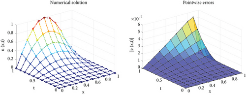
We solved this problem numerically using the polynomial spectral scheme provided in this paper. We employed fsolve in Matlab to solve a nonlinear system of equations (45). Table 1 shows the absolute errors for α = 0.5 and various β values. We can observe from this table that the recommended strategy is effective. Also, we portrayed the numerical solution and absolute error surfaces in Figure 1. Furthermore, the norm of errors and CPU times is reported in Table 2. Table 1, Table 2, and Figure 1 show that the numerical method provides acceptable results.

Example 2. Consider the following equation

(86)

with conditions (2) and (3). The source term is taken as

(87)

and

Table 1. Numerical reports in Example 1.

(ξ_i, η_i)	α = 0.5, K = 11	α = 0.5, K = 11	α = 0.5, K = 9	α = 0.5, K = 9
	β = 0.1, J = 4	β = 0.3, J = 4	β = 0.7, J = 4	β = 0.9, J = 4
(0.1,0.1)	5.2665e − 11	7.5026e − 11	9.4157e − 10	1.5935e − 09
(0.2,0.2)	8.8713e − 10	7.0142e − 10	1.7084e − 09	4.5505e − 09
(0.3,0.3)	4.6062e − 09	3.6713e − 09	5.8173e − 08	1.3764e − 09
(0.4,0.4)	1.4766e − 08	1.2353e − 08	3.6620e − 07	1.2902e − 07
(0.5,0.5)	3.6426e − 08	3.1853e − 08	1.2736e − 06	6.7104e − 07
(0.6,0.6)	7.6243e − 08	6.9345e − 08	3.4065e − 06	2.2596e − 06
(0.7,0.7)	1.4258e − 07	1.3432e − 07	7.7630e − 06	6.0393e − 06
(0.8,0.8)	2.4555e − 07	2.3833e − 07	1.5689e − 05	1.3673e − 05
(0.9,0.9)	3.8165e − 07	3.7801e − 07	2.5814e − 05	2.4145e − 05
(1, 1)	7.3344e − 15	1.1944e − 16	1.6793e − 15	2.1690e − 14

Details are in the caption following the image — **Figure 1**
Open in figure viewer PowerPoint

Pictorial results in Example 1 with α = 0.5, β = 0.1, and N = 11, M = 4.

Table 2. Norm of errors for α = β = 0.5 and CPU time in Example 1.

	J = 4, K = 6	J = 4, K = 7	J = 4, K = 8	J = 4, K = 9	J = 4, K = 10
	‖e‖_∞	‖e‖_∞	‖e‖_∞	‖e‖_∞	‖e‖_∞
	1.7427e − 03	1.7093e − 03	3.7497e − 05	3.7046e − 05	5.5452e − 07
CPU	0.7787s	1.3037s	1.4066s	1.5607s	1.9541s

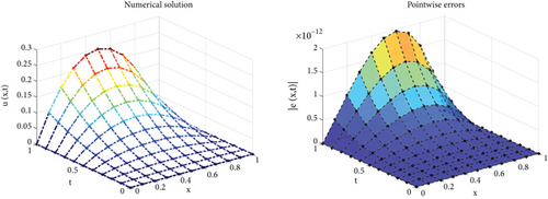
The absolute errors for equal values of α, β, and K = J = 3 are illustrated in Table 3. This table shows quite revealingly that the expressed method has good precision. In addition, we can observe from the table that only a small number of basis functions have produced the necessary outcomes. The CPU times and the norm of errors are provided in Table 4. Figure 2 shows a visualization of the approximate solution as well as absolute errors.

Example 3. Consider the following equation on [0, 1] × [0, 1]:

(88)

with conditions (2) and (3). The source term is taken as

(89)

Table 3. Numerical results in Example 2.

(ξ_i, η_i)	α = 0.5	α = 0.7	α = 0.9	α = 1
	β = 0.5	β = 0.5	β = 0.5	β = 0.5
(0, 0)	1.3878e − 17	1.3878e − 17	1.3878e − 17	6.9389e − 17
(0.1,0.1)	2.9677e − 15	2.4715e − 15	2.1732e − 15	2.4820e − 15
(0.2,0.2)	1.3601e − 14	1.0819e − 14	8.4386e − 15	8.1749e − 15
(0.3,0.3)	4.2369e − 14	3.3196e − 14	2.4869e − 14	2.1178e − 14
(0.4,0.4)	1.0748e − 13	8.5140e − 14	6.4282e − 14	5.2874e − 14
(0.5,0.5)	2.2699e − 13	1.8235e − 13	1.4061e − 13	1.1730e − 13
(0.6,0.6)	4.0491e − 13	3.2892e − 13	2.5840e − 13	2.2102e − 13
(0.7,0.7)	6.1083e − 13	5.0086e − 13	3.9917e − 13	3.4946e − 13
(0.8,0.8)	7.5499e − 13	6.2282e − 13	5.0181e − 13	4.4802e − 13
(0.9,0.9)	6.5503e − 13	5.4298e − 13	4.4097e − 13	4.0014e − 13
(1, 1)	7.5493e − 16	3.3867e − 16	1.0991e − 15	1.0437e − 15

Table 4. Norm of errors for α = β = 0.5 and CPU time in Example 2.

	J = 3, K = 3	J = 3, K = 4	J = 3, K = 5	J = 3, K = 6	J = 3, K = 7
	‖e‖_∞	‖e‖_∞	‖e‖_∞	‖e‖_∞	‖e‖_∞
	1.9604e − 12	4.9638e − 12	8.0466e − 11	1.3686e − 13	1.4568e − 12
CPU	0.7492s	0.9354s	1.1262s	1.2330s	1.2589s

The exact solution is .

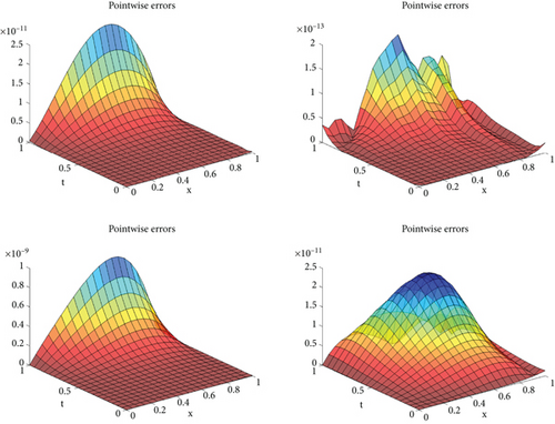
The numerical results are reported in Table 5. We have chosen K = 4, J = 5, and for equal α and β, the obtained results are fruitful. This table confirms that the presented method has high performance and produces accurate results. For α = β = 0.5 and different J and K, the norm of errors and the CPU times are provided in Table 3. The absolute error functions for equal α and β are sketched in Figure 3. These figures show that the numerical and exact solutions are almost identical (Table 6).

Example 4. Consider the following equation:

(90)

with conditions (2), (3), and

(91)

Table 5. Numerical results in Example 3.

(ξ_i, η_i)	α = 0.1	α = 0.4	α = 0.6	α = 0.8
	β = 0.1	β = 0.4	β = 0.6	β = 0.8
(0, 0)	4.7184e − 14	3.4972e − 15	5.5511e − 15	3.9191e − 14
(0.1,0.1)	3.0197e − 14	1.8513e − 17	9.9751e − 13	5.3904e − 14
(0.2,0.2)	9.1656e − 14	1.8249e − 15	3.8079e − 12	1.1759e − 12
(0.3,0.3)	1.9482e − 13	2.8203e − 15	8.9047e − 12	3.4628e − 12
(0.4,0.4)	4.2674e − 13	7.0777e − 15	1.8213e − 11	6.6157e − 12
(0.5,0.5)	9.4080e − 13	1.0436e − 14	3.9364e − 11	1.0878e − 11
(0.6,0.6)	1.9982e − 12	3.2196e − 14	8.7362e − 11	1.6063e − 11
(0.7,0.7)	3.9228e − 12	4.3965e − 14	1.7459e − 10	1.9690e − 11
(0.8,0.8)	6.4684e − 12	8.2379e − 14	2.8359e − 10	1.6850e − 10
(0.9,0.9)	7.9272e − 12	6.1506e − 14	3.2058e − 10	5.0651e − 12
(1, 1)	5.7618e − 12	8.9421e − 14	5.1744e − 11	3.9714e − 12

Table 6. Norm of errors for α = β = 0.5 and CPU time in Example 3.

	J = 5, K = 4	J = 5, K = 5	J = 5, K = 6	J = 5, K = 7	J = 5, K = 8
	‖e‖_∞	‖e‖_∞	‖e‖_∞	‖e‖_∞	‖e‖_∞
	1.7474e − 13	4.6830e − 10	5.1812e − 10	2.2715e − 09	3.7225e − 08
CPU	0.6941s	1.4075s	1.4990s	1.7516s	2.1537s

The exact solution is .

The absolute errors for α = β = 0.5 are presented in Table 7. Table 8 illustrates the norm of errors and CPU times for α = β = 0.5 with various J and K values. Table 9 also contains data on L₂ errors. Numerical solutions and pointwise error graphs are demonstrated in Figure 4. This figure shows the behavior of the numerical solution and the error function. Numerical results are in good settlement with theoretical results.

Example 5. Finally, we investigate the following equation on [0, 1] × [0, 1]

(92)

with conditions (2) and (3). The source term is taken as

(93)

and

Table 7. Numerical reports in Example 4.

(ξ_i, η_i)	J = 4	J = 4	J = 4	J = 4
	K = 6	K = 7	K = 8	K = 9
(0, 0)	3.9549e − 20	1.9230e − 22	6.7320e − 20	1.1194e − 18
(0.1,0.1)	1.0519e − 10	5.3038e − 12	4.6608e − 13	2.8112e − 12
(0.2,0.2)	2.7128e − 09	1.4373e − 10	7.5190e − 12	8.1029e − 12
(0.3,0.3)	2.6072e − 08	1.4112e − 09	6.8470e − 11	1.6060e − 11
(0.4,0.4)	1.0383e − 07	5.6159e − 09	2.7027e − 10	3.5035e − 11
(0.5,0.5)	2.8045e − 07	1.5208e − 08	7.3186e − 10	8.5052e − 11
(0.6,0.6)	6.1575e − 07	3.3347e − 08	1.6119e − 09	1.9935e − 10
(0.7,0.7)	1.2047e − 06	6.5140e − 08	3.1553e − 09	4.1556e − 10
(0.8,0.8)	2.1149e − 06	1.1777e − 07	5.7928e − 09	7.3660e − 10
(0.9,0.9)	2.8168e − 06	1.7066e − 07	8.9641e − 09	9.7501e − 10
(1, 1)	1.3234e − 14	2.6645e − 15	1.0658e − 14	3.5527e − 15

Table 8. Norm of errors for α = β = 0.5 and CPU time in Example 4.

	J = 4, K = 5	J = 4, K = 6	J = 4, K = 7	J = 4, K = 8	J = 4, K = 9
	‖e‖_∞	‖e‖_∞	‖e‖_∞	‖e‖_∞	\| ‖e‖_∞
	5.4599e − 05	3.6853e − 06	2.2397e − 07	1.1841e − 08	1.2327e − 09
CPU	0.6648s	1.3185s	1.2689s	1.3789s	1.5100s

Table 9. Norm of errors for α = 0.5, β = 0.5 in Example 4.

J	K	‖e‖₂
4	5	3.0728e − 05
4	6	2.0621e − 06
4	7	1.1742e − 07
4	8	6.0069e − 09
4	9	7.7425e − 10

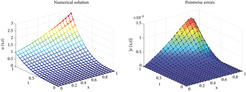
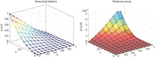
In Table 10, the L₂ error is computed for α = β = 0.5 and different N and M. Table 11 also shows the norm of errors and CPU times. Figure 5 shows the numerical solution and absolute error plots. This figure shows that for K = 9 and J = 4, the numerical solution is close to the exact solution. Table 10, Table 11, and Figure 5 affirm the validity and efficacy of the presented method.

Table 10. Norm of errors for α = 0.5, β = 0.5 in Example 5.

		α = β = 0.3	α = β = 0.5	α = β = 0.7	α = β = 0.9
J	K	‖e‖₂	‖e‖₂	‖e‖₂	‖e‖₂
3	5	7.2576e − 05	7.1011e − 05	7.1448e − 05	6.0514e − 05
3	6	1.5363e − 05	1.5000e − 05	1.4978e − 05	1.3806e − 05
3	7	3.8656e − 07	3.7824e − 07	3.7609e − 07	3.4637e − 07
3	8	5.1965e − 08	5.0757e − 08	5.0432e − 08	3.9225e − 08
3	9	1.1091e − 09	2.4799e − 09	1.6532e − 08	6.7070e − 08

Table 11. Norm of errors for α = β = 0.5 and CPU time in Example 5.

	J = 3, K = 5	J = 3, K = 6	J = 3, K = 7	J = 3, K = 8	J = 3, K = 9
	‖e‖_∞	‖e‖_∞	‖e‖_∞	‖e‖_∞	\| ‖e‖_∞
	1.1228e − 04	2.3945e − 05	6.0186e − 07	8.0155e − 08	4.0315e − 09
CPU	0.5944s	1.0808s	1.1061s	1.1594s	1.2277s

6. Conclusions

The purpose of this study was to suggest a collocation approach for solving a nonlinear TFPIDE based on Pell polynomials. In the Caputo sense, the fractional derivative is considered. The equation’s solution was expressed as a series of Pell polynomials with two variables. An algebraic system of nonlinear equations is obtained using the numerical technique. We proved that the method is convergent. Five test problems are provided to show that the method is efficacious. In numerical results, a small number of basis Pell polynomials is used to obtain good accuracy. In all examples, the CPU time was about one second. All of the tables and graphs demonstrated that the strategy is effective.

Conflicts of Interest

The authors declare that they have no conflicts of interest.

Open Research

Data Availability

All results have been obtained by conducting the numerical procedure and the ideas can be shared for the researchers.

References

1 Dutta H., Akdemir A., and Atangana A., Fractional Order Analysis: Theory, Methods and Applications, 2020, John Wiley and Sons Ltd, https://doi.org/10.1002/9781119654223.
10.1002/9781119654223
Google Scholar
2 Kumar D. and Singh J., Fractional Calculus in Medical and Health Science, 2020, Taylor & Francis Group, LLC.
10.1201/9780429340567
Google Scholar
3 Anastassiou G. A., Generalized Fractional Calculus: New Advancements and Applications, 2020, Springer.
Google Scholar
4 Trigeassou J. C. and Maamri N., Analysis, Modeling and Stability of Fractional Order Differential Systems 2, 2019, John Wiley & Sons, https://doi.org/10.1002/9781119686859.
Google Scholar
5 Caponetto R., Dongola G., Fortuna I., and Petras I., Fractional Order Systems: Modeling and Control Applications, 2010, World Scientific, https://doi.org/10.1142/7709.
10.1142/7709
Google Scholar
6 Matouk A. E., Advanced applications of fractional differential operators to science and technology, IGI Global. (2020) https://doi.org/10.4018/978-1-7998-3122-8.
10.4018/978-1-7998-3122-8
Google Scholar
7 Baleanu D. and Lopes A. M., Handbook of Fractional Calculus with Applications, Volume 7 Applications in Engineering, 2019, Life and Social Sciences, Part A, de Gruyter.
Google Scholar
8 Yang X. J., Gao F., and Ju Y., General Fractional Derivatives with Applications in Viscoelasticity, 2020, Academic Press, https://doi.org/10.1016/B978-0-12-817208-7.00011-X.
Google Scholar
9 Shishkina E. and Sitnik S., Transmutations, Singular and Fractional Differential Equations with Applications to Mathematical Physics, 2020, Academic Press, https://doi.org/10.1016/B978-0-12-819781-3.00017-3.
Google Scholar
10 Atangana A., Fractional Operators with Constant and Variable Order with Application to Geo-Hydrology, 2017, Academic Press.
Google Scholar
11 Valerio D. and Ortigueira M. D., Fractional Signals and Systems, 2020, de Gruyter, https://doi.org/10.1515/9783110624588.
Google Scholar
12 Meerschaert M. M. and Sikorskii A., Stochastic Models for Fractional Calculus, 2019, de Gruyter, https://doi.org/10.1515/9783110560244.
Google Scholar
13 Ostalczyk P., Sankowski D., and Nowakowski J., On-Integer Order Calculus and Its Applications, 2019, Springer.
10.1007/978-3-319-78458-8
Google Scholar
14 Fallahgoul H., Focardi S., and Fabozzi F., Fractional Calculus and Fractional Processes with Applications to Financial Economics: Theory and Application, 2017, Academic Press.
Google Scholar
15 Sun Z. Z. and Gao G., Fractional Differential Equations: Finite Difference Methods, 2020, Walter de Gruyter GmbH & Co KG, https://doi.org/10.1515/9783110616064.
10.1515/9783110616064
Google Scholar
16 Li C. and Zeng F., Numerical Methods for Fractional Calculus, 2019, Chapman and Hall/CRC.
Google Scholar
17 Abd-Elhameed W. M. and Youssri Y. H., Sixth-kind Chebyshev spectral approach for solving fractional differential equations, Int. J. Nonlin. Sci. Num.(2019) 20, no. 2, 191–203, https://doi.org/10.1515/ijnsns-2018-0118, 2-s2.0-85064165366.
10.1515/ijnsns-2018-0118
Web of Science® Google Scholar
18 Abd-Elhameed W. M., Novel expressions for the derivatives of sixth kind Chebyshev polynomials: spectral solution of the non-linear one-dimensional Burgers’ equation, Fractal and Fractional. (2021) 5, no. 2, https://doi.org/10.3390/fractalfract5020053.
10.3390/fractalfract5020053
PubMed Web of Science® Google Scholar
19 Abd-Elhameed W. M. and Youssri Y. H., New formulas of the high-order derivatives of fifth-kind Chebyshev polynomials: spectral solution of the convectionâ€’diffusion equation, Numerical Methods for Partial Differential Equations. (2021) 1–17, https://doi.org/10.1002/num.22756.
10.1002/num.22756
Web of Science® Google Scholar
20 Samiee M., Kharazmi E., Meerschaert M. M., and Zayernouri M., A unified Petrov–Galerkin spectral method and fast solver for distributed-order partial differential equations, Communications on Applied Mathematics and Computation. (2021) 3, no. 1, 61–90, https://doi.org/10.1007/s42967-020-00070-w.
10.1007/s42967-020-00070-w
Google Scholar
21 Jani M., Babolian E., and Bhatta D., A Petrov–Galerkin spectral method for the numerical simulation and analysis of fractional anomalous diffusion, Mathematical Methods in the Applied Sciences. (2021) 44, no. 2, 2021–2032, https://doi.org/10.1002/mma.6908.
10.1002/mma.6908
Web of Science® Google Scholar
22 Guo B., Pu X., and Huang F., Fractional Partial Differential Equations and Their Numerical Solutions, 2015, World Scientific, https://doi.org/10.1142/9543.
10.1142/9543
Google Scholar
23 Ray S. S., Nonlinear Differential Equations in Physics: Novel Methods for Finding Solutions, 2020, Springer.
Google Scholar
24 Wang H., Xu D., Zhou J., and Guo J., Weak Galerkin finite element method for a class of time fractional generalized Burgers' equation, Numerical Methods for Partial Differential Equations. (2021) 37, no. 1, 732–749, https://doi.org/10.1002/num.22549.
10.1002/num.22549
Web of Science® Google Scholar
25 Zheng Y. and Zhao Z., The time discontinuous space-time finite element method for fractional diffusion-wave equation, Applied Numerical Mathematics. (2020) 150, 105–116, https://doi.org/10.1016/j.apnum.2019.09.007, 2-s2.0-85072636494.
10.1016/j.apnum.2019.09.007
Web of Science® Google Scholar
26 Dehghan M., Manafian J., and Saadatmandi A., Solving nonlinear fractional partial differential equations using the homotopy analysis method, International Journal. (2010) 26, no. 2, 448–479, https://doi.org/10.1002/num.20460, 2-s2.0-76649094637.
10.1002/num.20460
Google Scholar
27 Nikan O., Avazzadeh Z., and Machado J. A. T., An efficient local meshless approach for solving nonlinear time-fractional fourth-order diffusion model, Journal of King Saud University-Science. (2021) 33, no. 1, article 101243, https://doi.org/10.1016/j.jksus.2020.101243.
10.1016/j.jksus.2020.101243
Web of Science® Google Scholar
28 Safari F. and Azarsa P., Backward substitution method based on Müntz polynomials for solving the nonlinear space fractional partial differential equations, Mathematical Methods in the Applied Sciences. (2020) 43, no. 2, 847–864, https://doi.org/10.1002/mma.5963.
10.1002/mma.5963
Web of Science® Google Scholar
29 Yaslan H. C., Legendre collocation method for the nonlinear space–time fractional partial differential equations, Iranian Journal of Science and Technology, Transactions A: Science. (2020) 44, no. 1, 239–249, https://doi.org/10.1007/s40995-020-00824-4.
10.1007/s40995-020-00824-4
Web of Science® Google Scholar
30 Shen J., Tang T., and Wang L. L., Spectral Methods: Algorithms, Analysis and Applications, 2011, Springer Science & Business Media, https://doi.org/10.1007/978-3-540-71041-7.
10.1007/978-3-540-71041-7
Web of Science® Google Scholar
31 Canuto C., Hussaini M. Y., Quarteroni A., and Zang T. A., Spectral Methods in Fluid Dynamics, 2012, Springer Science & Business Media.
Google Scholar
32 Agarwal P., El-Sayed A. A., and Tariboon J., Vieta-Fibonacci operational matrices for spectral solutions of variable-order fractional integro-differential equations, Journal of Computational and Applied Mathematics. (2021) 382, article 113063, https://doi.org/10.1016/j.cam.2020.113063.
10.1016/j.cam.2020.113063
Web of Science® Google Scholar
33 Moshtaghi N. and Saadatmandi A., Polynomial-Sinc collocation method combined with the Legendre-Gauss quadrature rule for numerical solution of distributed order fractional differential equations, Revista de la Real Academia de Ciencias Exactas, FÃsicas y Naturales. Serie A. MatemÃ¡ticas. (2021) 115, no. 2, 1–23, https://doi.org/10.1007/s13398-020-00976-3.
10.1007/s13398-020-00976-3
Web of Science® Google Scholar
34 Abbaszadeh M., Dehghan M., and Zhou Y., Crank-Nicolson/Galerkin spectral method for solving two-dimensional time-space distributed-order weakly singular integro-partial differential equation, Journal of Computational and Applied Mathematics. (2020) 374, article 112739, https://doi.org/10.1016/j.cam.2020.112739.
10.1016/j.cam.2020.112739
Web of Science® Google Scholar
35 Zheng X., Qiu W., and Chen H., Three semi-implicit compact finite difference schemes for the nonlinear partial integro-differential equation arising from viscoelasticity, International Journal of Modelli ng and Simulation. (2021) 41, no. 3, 234–242, https://doi.org/10.1080/02286203.2020.1720566.
10.1080/02286203.2020.1720566
Web of Science® Google Scholar
36 Sanz-Serna J. M., A numerical method for a partial integro-differential equation, SIAM Journal on Numerical Analysis. (1988) 25, no. 2, 319–327, https://doi.org/10.1137/0725022.
10.1137/0725022
Web of Science® Google Scholar
37 Guo J., Xu D., and Qiu W., A finite difference scheme for the nonlinear time–fractional partial integro–differential equation, The European Physical Journal Plus. (2021) 136, no. 1, 1–30.
Google Scholar
38 Atta A. G., Moatimid G. M., and Youssri Y. H., Generalized Fibonacci operational collocation approach for fractional initial value problems, International Journal of Applied and Computational Mathematics. (2019) 5, no. 1, 1–11, https://doi.org/10.1007/s40819-018-0597-4, 2-s2.0-85061991015.
10.1007/s40819-018-0597-4
Google Scholar
39 Atta A. G., Abd-Elhameed W. M., Moatimid G. M., and Youssri Y. H., Shifted fifth-kind Chebyshev Galerkin treatment for linear hyperbolic first- order partial differential equations, Applied Numerical Mathematics. (2021) 167, 237–256, https://doi.org/10.1016/j.apnum.2021.05.010.
10.1016/j.apnum.2021.05.010
Web of Science® Google Scholar
40 Atta A. G., Moatimid G. M., and Youssri Y. H., Generalized Fibonacci operational tau algorithm for fractional Bagley-Torvik equation, Prog. Fract. Differ. Appl. (2020) 6, no. 3, 215–224, https://doi.org/10.18576/pfda/060305.
10.18576/pfda/060305
Google Scholar
41 Taghipour M. and Aminikhah H., Application of Pell collocation method for solving the general form of time-fractional burgers equations, Mathematical Sciences. (2022) 1-19, https://doi.org/10.1007/s40096-021-00452-y.
10.1007/s40096-021-00452-y
Google Scholar
42 Horadam A. F. and Mahon J. M., Pell and Pell-Lucas polynomials, The Fibonacci Quarterly. (1985) 23, no. 1, 7–20.
Web of Science® Google Scholar
43 Abd-Elhameed W. M. and Youssri Y. H., Spectral tau algorithm for certain coupled system of fractional differential equations via generalized Fibonacci polynomial sequence, Iranian Journal of Science and Technology, Transactions A: Science. (2019) 43, no. 2, 543–554, https://doi.org/10.1007/s40995-017-0420-9, 2-s2.0-85061035962.
10.1007/s40995-017-0420-9
Web of Science® Google Scholar
44 Abd-Elhameed W. M. and Youssri Y. H., Generalized Lucas polynomial sequence approach for fractional differential equations, Nonlinear Dynamics. (2017) 89, no. 2, 1341–1355, https://doi.org/10.1007/s11071-017-3519-9, 2-s2.0-85017193890.
10.1007/s11071-017-3519-9
Web of Science® Google Scholar
45 Callahan J. J., Advanced Calculus: A Geometric View, 2010, Springer Science & Business Media, https://doi.org/10.1007/978-1-4419-7332-0.
10.1007/978-1-4419-7332-0
Google Scholar
46 Youssri Y. H., A new operational matrix of Caputo fractional derivatives of Fermat polynomials: an application for solving the Bagley-Torvik equation, Adv. Difference Equ.(2017) 2017, no. 1, 1–17, https://doi.org/10.1186/s13662-017-1123-4, 2-s2.0-85014548590.
10.1186/s13662-017-1123-4
Web of Science® Google Scholar
47 Byrd P. F., Expansion of analytic functions in polynomials associated with Fibonacci numbers, Fibonacci Q.(1963) 1, article n16.
Google Scholar
48 Taghipour M. and Aminikhah H., A fast collocation method for solving the weakly singular fractional integro-differential equation, Computational and Applied Mathematics. (2022) 41, no. 4, https://doi.org/10.1007/s40314-022-01845-y.
10.1007/s40314-022-01845-y
Web of Science® Google Scholar
49 Jameson G. J. O., The incomplete gamma functions, The Mathematical Gazette. (2016) 100, no. 548, 298–306, https://doi.org/10.1017/mag.2016.67.
10.1017/mag.2016.67
Web of Science® Google Scholar

Citing Literature

All articles

Pell Collocation Method for Solving the Nonlinear Time–Fractional Partial Integro–Differential Equation with a Weakly Singular Kernel

Abstract

1. Introduction

2. Definitions

3. Analysis of the Numerical Method

4. Convergence

5. Numerical Experiments

6. Conclusions

Conflicts of Interest

Open Research

Data Availability

References

Citing Literature

Figures

References

Information

About Wiley Online Library

Help & Support

Opportunities

Connect with Wiley

Pell Collocation Method for Solving the Nonlinear Time–Fractional Partial Integro–Differential Equation with a Weakly Singular Kernel

Abstract

1. Introduction

2. Definitions

3. Analysis of the Numerical Method

4. Convergence

5. Numerical Experiments

6. Conclusions

Conflicts of Interest

Open Research

Data Availability

References

Citing Literature

Figures

References

Related

Information