This paper gives a detailed introduction of implementing mixture of Gaussian process (MGP) model and develops its application for Bayesian optimization (BayesOpt). The paper also develops techniques for MGP in finding its mixture components and introduced an alternative gating network based on the Dirichlet distributions. BayesOpt using the resultant MGP model significantly outperforms the one based on Gaussian process regression in terms of optimization efficiency in the test on tuning the hyperparameters in common machine learning algorithms. This indicates the success of the methods, implying a promising future of wider application for MGP model and the BayesOpt based on it.

1. Introduction

Bayesian optimization (BayesOpt) is a highly effective method for optimizing expensive black-box objective functions. These functions are expensive to evaluate and cannot be accessed analytically due to their complicated structures. They often come along with properties such as being noisy and having multiple local optima. Simple approaches like random search are inappropriate, and derivative-based algorithms like gradient decent are unreliable as well as inefficient due to the noisy and expensive nature of the objective functions. To address these issues, BayesOpt offers a derivative-free approach by building a surrogate that models the objective function and deciding where to evaluate using Bayesian statistics [1–3]. The ability to optimize expensive black-box derivative-free functions brought BayesOpt a wide range of applications since the 1960s [4, 5]. It is extensively used for designing engineering systems in robotics, computer graphics, and sensor networks [6–8], and it has recently become extremely popular for tuning hyperparameters in machine learning algorithms [9, 10].

BayesOpt is a member of the surrogate modelling methods in nature. The central idea behind this more general class of method is to use a well-behaved function that estimates the objective function based on a limited number of sampled data while being cheap to evaluate [11, 12]. The mostly used surrogate in BayesOpt is Gaussian process regression (GPR) [13]. It uses a set of parameters in its covariance function (kernel) to characterize the fluctuation of the objective function and makes regression using Bayes’ theorem. When combined with other methods to help finding the parameters in its kernel, GPR provides satisfying result. But it can be further improved by generalizing to the mixture of Gaussian process (MGP) model. The main motivation of this generalization is that the objective function’s behaviour is most likely inconsistent throughout the input space; hence, a single GPR with a fixed set of kernel parameters is typically inadequate for modelling the entire objective function. The MGP model overcomes this problem by self-organizing several GPs with different kernel parameters, allowing the kernel to be input-dependent [14].

The MGP model is a variant of the well-known mixture of expert (ME) model of Jacobs et al. [15] and was firstly introduced in Tresp [14]. It is a mixture model consisting of an input-dependent gating network and several GPs as the mixture components. Each GP specializes in a certain region of the input space due to their unique kernel parameters and stands for the local expert in the ME model. The gating network learns the specialization of the experts from the training data and estimates the participation of each expert for a new input. With this mechanism, the MGP model divides up the regression of the entire objective function into several regional subtasks to be executed by each expert, respectively, achieving a better overall result than any individual GPR [14]. By substituting GPR with MGP as the surrogate model, BayesOpt can more accurately estimate the objective function, speeding up its convergence on finding the optimum.

This paper firstly gives a brief review of the BayesOpt using GPR and then provides a detailed description of the MGP model with an alternative gating network modified from Rasmussen and Ghahramani [16] along with the method to find the local experts. Based on the discussions in the previous sections, a clustering-assisted approach to implement the MGP in the BayesOpt is introduced. Finally, the performance of the MGP model and the BayesOpt based on it are tested and discussed.

2. Background Review

2.1. Gaussian Process Regression

Gaussian process regression (GPR) is the most commonly used surrogate regression model in BayesOpt. It uses Gaussian process (GP) to build up the statistical inference, assuming the values of the objective function forming a multivariable Gaussian distribution with a particular mean vector and covariance matrix [17].

(1)

The term denotes the mean vector, which is commonly chosen to be a constant value, typically zero or the average of the sampled values. Matrix Σ is the covariance matrix, generated by a covariance function also known as kernel. The kernel models the correlation between each pair of points based on their positions. The mean vector together with kernel completely defines the properties of the GP [18, 19].

Following the fact that points that are closer in the input space typically have stronger correlations, the kernel value is always positive and decreases asymptotically to zero as the spatial distance increases. There are two major two types of kernels. The first type is Gaussian kernel (also called power exponential), where the correlation decreases in the form of a Gaussian function.

(2)

The term α₀ is the variance of the function’s values in the prior, and ‖x − x^′‖ is the metric in the input space. Such metric is not necessarily isotropic and Euclidean and typically takes in the form

, where the l_1:d in the denominators are called length scales. The second type is called Matérn kernel which takes in the following form [20]:

(3)

where Γ is the gamma function and K_v is the modified Bessel function of the second kind. The additional positive parameter v characterizes the smoothness of the regression model as GPs based on Matérn kernel are ⌈v⌉ − 1 times differentiable in the mean-square sense [20, 21]. Additionally, in the limit where v tends to infinity, the Matérn kernel converges to Gaussian kernel, which corresponds to the fact that GPs with Gaussian kernel are infinitely differentiable. In practice, Gaussian kernel could overestimate the smoothness of the objective function; hence, Matérn kernel is often used in the cases where the differentiability of the objective function is known or assumed to a certain degree.

In the cases where measurements are noisy, the kernels above still hold for any pairs of points that are distinct (namely, x ≠ x^′) as noises do not contribute to correlation. The variances however are increased by the variance of the noise. Hence, the covariance matrix can be expressed in the following form [20], where

is the variance of the noise.

(4)

To make regression, GPR firstly combines the sampled points along with the point to evaluate into a GP as the prior distribution. Then, the evaluation is done by finding the posterior distribution of the value to evaluate given the sampled data points according to Bayes’ theorem. The resultant posterior distribution can be derived from (1) and is presented below [20, 22]:

(5)

(6)

(7)

2.2. Choosing Kernel Parameters

The parameters in the kernel of GPR, especially the length scales, greatly affect the performance of regression. The length scales characterize the inverse speed that the function changes along each axis. A small length scale indicates the function changes rapidly along this axis, while a large length scale assumes the function is flatter and smoother. Based on different assumptions hence different length scales, the regression gives out distinct results as illustrated in Figure 1. If one assumes the actual function is well represented by the sampled points, the length scales can be chosen using maximum likelihood estimation (MLE). In this approach, the length scales are the configuration that maximizes the likelihood of the observations under the prior [23], namely,

(8)

Details are in the caption following the image — **Figure 1**
Open in figure viewer PowerPoint

The regressions made on the same function using different length scales. The regression value is taken to be the mean of the posterior distribution.

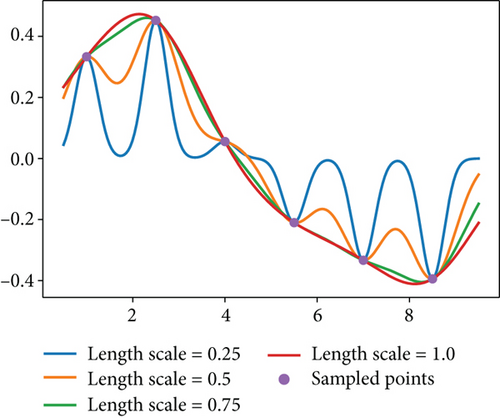
The length scales found are anisotropic in general. One can also assume the length scales to be isotropic, meaning that the same length scale is shared for all axes and MLE degenerates to maximizing . Such assumption is obviously less comprehensive but more appropriate when there are relatively few sampled points. It is especially the case when the number of sampled points is not significantly larger than the dimension of the input space, since the assumption for the function being well-represented breaks down and MLE could fall into overfitting. Typically, the objective function is randomly sampled a few times before using BayesOpt to meet the minimum requirement for applying GPR. It is also suggested to use isotropic GPR before having enough points to apply the anisotropic GPR.

2.3. Acquisition Function

After finding the posterior distribution of the objective function, BayesOpt uses an acquisition function to evaluate how desirable it is to sample at this position. Two types of most commonly used acquisition functions are the probability of improvement (PI) [24] and the expected improvement (EI) [25]. PI calculates the probability of finding a value better than the current optimum based on the posterior distribution found by GPR. EI modifies PI by taking into account the scale of the potential improvement but could favour explorative sampling as it does not account for the risk. According to the experiment carried out by Wu et al. [26], EI overall outperforms PI in finding global optimum; hence, it is the acquisition function chosen for this paper. The EI is defined as follows [25]:

(9)

where y_∗ denotes the current optimal value and f(y) is the probability density of the posterior distribution given by the surrogate regression model. One may combine this with (5) to evaluate EI in closed form as described in Clark [27]:

(10)

where z = (μ_∗(x) − y_∗)/(σ_∗(x)) (or (y_∗ − μ_∗(x))/(σ_∗(x)) if to minimize). The point to sample next is the one that maximizes the acquisition function. After sampling, the GPR and the acquisition function are updated by taking into the new data point. This process is repeated for a certain number of iterations, and the final optimum is the best point among the sampled dataset.

2.4. Mixture of Gaussian Processes

GPR uses a certain configuration of kernel parameters typically optimized via MLE, assuming a global behaviour of the function in each dimension. In most cases, this is inadequate to model the entire objective function, as the function typically has different behaviours in different regions. For example, the objective function could have one local peak that changes quickly on x-axis but slowly on y-axis and another one elsewhere that behaves in reverse, or the objective function could be a single hump surrounded by a vast flat region. The main motivation for replacing GPR by the mixture of Gaussian process (MGP) model is to address these scenarios by permitting input-dependent participation of kernel parameters. The MGP model is a variation of mixture of expert (ME) model and a generalization of GPR. It consists of a set of GPs with different kernel parameters as the experts and a gating network to determine which expert to use for a given input [15]. The gating network and the mixture components are iteratively trained using the expectation maximization (EM) algorithm to maximize the likelihood of the observed data. Compared with the original method introduced in Tresp [14], the MGP model introduced in this paper is slightly modified for better performance.

2.5. Finding the Local Experts

The method for finding the experts is not specified in Tresp [14]. To account for the fact that the function’s behaviour is regional, it is desirable to find the local experts that are optimized for certain regions. Here, the modified maximum likelihood estimation approach is introduced to find the experts. For each region

to optimize, the whole dataset is divided into two groups, the points that are within the region

and the ones that are not

. The kernel parameters for the local GPR are the set that maximizes the probability of finding the data points within this region conditioned on the rest data points, namely,

(11)

which is to maximize the likelihood of the regional observations under the posterior. This is a reasonable method as the experts in the MGP model make regressions based on the whole dataset, and the GPR optimized from (11) corresponds to the expert that most accurately predicts the local data. When the region covers the entire dataset, (11) degenerates to (8) and the method becomes MLE.

The regions to generate the local experts are not necessarily mutually exclusive as the gating network will assign the tasks automatically. However, they are expected to be exhaustive since otherwise the regressions in the uncovered area could result badly. A simple approach to fulfill this requirement is to use the GPR optimized via MLE (such GPR will be referred to as global GPR for the rest of this paper) along with the ones optimized for certain regions. Finally, to avoid overfitting, one has to make sure the regions to optimize are well-shaped and contain enough points.

2.6. Iterative Learning Using EM

After finding the GP experts, the model is trained via an iterative learning using the EM algorithm. The EM consists of two steps, the E step for estimation and the M step for maximization. In the E step, based on the current form of the GPs, the latent variables for each data point are estimated using Bayes’ theorem:

(12)

where the discrete variable z denotes the membership of the GPs and notation G(a; b, c²) stands for the probability density of a Gaussian distribution with mean b and variance c² evaluated at a. A difference from the method in Tresp [14] is that the original paper used another set of GPs to model the variances of the posterior distributions, while (12) uses the variances calculated from (5). The original method has some merit, but (12) is computationally cheaper and theoretically more legitimate. Unlike the EM for the Gaussian mixture model, the prior probability of the latent variable is estimated by the gating network instead of the mixture weights. The term p(z = i|x_k) is the estimated probability of the regression task being assigned to the i^th expert evaluated by the gating network at x_k. In the M step, the gating network and the GPs are updated based on the results calculated in the E step to maximize the likelihood. While the procedure to update the gating network will be introduced later, the update of the GPs is done by amplifying the noise variances on the diagonal of the covariance matrix according to the latent variables.

(13)

where Ψⁱ is a diagonal matrix with entries [14]:

(14)

The M step and the E step are conducted alternately until convergence.

However, there are some problems found during the implementation of the EM. The first one is mentioned in Tresp [14] that calculating the probability density on known data points could lead to serious overtraining. This problem is solved by using all the training data except (x_k, y_k) when calculating (12). However, this leads to the second problem of numerical instability as the predicted value could be tens of standard deviations away from the true value for some GPRs and the probability densities become indistinguishable from zero for the computer. This problem can be solved by using approximations such as the Taylor expansion to provide accurate results for good regressions while keeping it computable for bad regressions. Another problem is that the EM does not guarantee to converge. This is understandable as EM is a maximum likelihood estimation for the mixture model in nature, and it could be oscillating between two points having similar likelihood [28]. To address this problem, one could calculate the logarithm of the posterior density for each EM iteration:

(15)

If the EM still does not converge after a certain number of iterations, simply choose the iteration step that corresponds to the highest posterior density.

3. Methodology

3.1. Learning the Alternative Gating Network

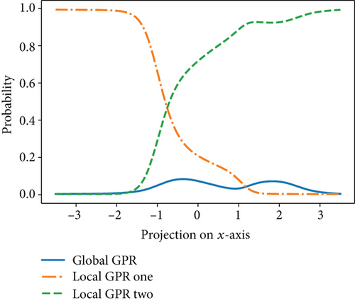
The gating function in ME model evaluates the expert-membership of a new input by means of regression. In the original paper, this is done using Gaussian process classification [29] (GPC) with a softmax function. This method is found to be not ideal enough. One reason is that GPC requires to label the expert-memberships for each data point, while some points have rather equivalent probabilities for several GPRs, making it inappropriate to label them with any model. Another problem originates from the fact that some data points, inside a region covered by a local GPR through, could fit very well to another GPR optimized for some other region. As a result, the situation that one data point that seemingly belongs to a GPR being surrounded by many data points that favour another GPR is likely a sign of this type of problem. Hence, it may be desirable to take into account the status of the surrounding data. The successful implementation of the original method was on functions that are rather steep, such as the step function in Tresp [14] and the spike-shaped function in Stachniss et al. [30], where the sudden change of label makes sense. However, for most functions, the original method could lead to wrong classification and hence is not very ideal. Also, a M-class GPC uses M GPRs to make regressions and is computationally rather expensive.

To address these problems, an alternative gating network modified from Rasmussen and Ghahramani [16] is used. For each data point, the assignment probabilities are assumed to follow a symmetric Dirichlet distribution in the prior:

(16)

where the α/M is the concentration parameter and the probabilities π_j must be positive and sum to one. The prior probability to find the data points in a certain configuration of assignment can be calculated using the standard Dirichlet integral [31].

(17)

where c_i is the expert assignment, also called indicator variable, for the i^th data. The term N_j is the occupation number for the j^th expert, which is the number of data points assigned to this expert. Using (17), one can calculate the posterior probability distribution for a single indicator variable given the rest.

(18)

where the subscript −i denotes all indexes except for i. Note that the posterior does not take in any positional information; hence, a local estimation for the occupation number is used to construct the gating network. This is done by using a kernel smoother as in Rasmussen and Ghahramani [16] to give a higher weight to the neighbouring points.

(19)

(20)

A modification from Foster et al. [31] is that (19) uses the posterior distribution calculated from (12). This is to integrate the update of the gating network into the EM learning algorithm. This method successfully solves the problems found in the original gating network as it takes in the probabilities of the indicator variable as well as the surrounding data. The length scales ϕ in the kernel smoother characterizes the smoothness of the gating network. Optimizing the ϕ can be difficult as this could fall into overfitting. It is advised to preset an isotropic ϕ and to use the smoother on the data normalized in each dimension.

The α in the concentration parameter controls the prior distribution and hence influences the gating network. To account for the variation of α, one can use a Bayesian approach to find the posterior of α the and sample from this distribution. As the method introduced in Rasmussen [32], the prior of α is assumed to be an inverse gamma and its posterior takes in the following form:

(21)

where B(α, N) denotes the beta function. The sampling of the posterior can be made using the adaptive rejection sampling (ARS) method [33]. Allowing the α to vary makes the gating network more robust. However, the function (21) is not strictly log-concave at the tail end where the probability density is almost zero. One may need to make some approximations to deal with this.

3.2. Complete Algorithm of MGP

To sum up, one can successfully implement the MGP following the steps presented in Algorithm 1.

Algorithm 1: Training the MGP model.

Input: Sampled data, the regions to optimize, the term ϕ in the smoother.
1 Sample from the posterior of α using (21) and ARS.
2 Find the global GPR and the local experts using (11).
3 Initialize the gating network (equal probability for all experts is fine).
4 repeat
5 Calculate the probability densities for the data points under each GP.
6 Estimate the latent variables using (12).
7 Update the GPs using (13).
8 Update the gating network using (18).
9 /∗ The gating network is averaged over the sampled posterior of α∗/
10 Δ = the root-mean-square deviation of the updated gating network.
11 until Δ < tolerance;
Output: the trained GPs with the gating network.

For any input to evaluate, use (18) to calculate the assignment probabilities and then use (5) to make regressions for each GPR, respectively.

In practice, one may conduct EM until convergence without (13), which is to keep the GPs fixed, before applying the EM with (13). This is because recalculating the probability densities after updating the GPs is the most time-consuming step. Hence, a better gating network to begin with can significantly speed up the training. But above all, one needs to make sure there are enough data points to perform the MGP; otherwise, this can lead to overfitting.

3.3. Clustering-Assisted Method for BayesOpt

A major drawback of the MGP introduced above is that the local expert can only be designated if the regions to optimize are known. If the behaviour of the function is vaguely known in advance or if there are many sampled data points, one can select the regions manually. But for a general optimization task, this can be hard to do as little is known for the objective function and number of samplings is limited.

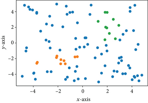
By studying general BayesOpt optimizations, one can find that the local experts that the optimizer is mostly interested in are the ones for the local peaks where the sampling density is high. Utilizing this feature, local experts to construct MGP for BayesOpt can be determined using a clustering-assisted approach. One firstly filters out the data with values below the average (or above the average if to minimize) and then applies density-based clustering to the rest points. The clustering step is advised to be conducted on data normalized in each input dimension. Each cluster found corresponds to a group of samplings around a local peak and the local experts can be found using (11). As the later samplings tend to lie around the higher peaks, the average of sampled values increases after each iteration. Thus, the lower peaks are of lesser value and will gradually be filtered out (once the cluster size is too small), leaving only the highest peak standing.

If there is no cluster found, meaning that the BayesOpt has not found any peak or there are not enough points near a peak to fit a local expert, the MGP uses only the global GPR which does not pose any adverse consequences either. The worst case that the clustering approach could lead to is finding a cluster in the filtered data points which turns out to be high value points mixed up with low value ones in the whole dataset. In this case, the GPR calculated via (11) does not reflect any regional behaviour of the function but is simply overlearning this subset of data. This is a rare scenario but is still worthy of attention. A solution addressing this issue is to make a k-nearest neighbour classification of the unselected data for each cluster. This grows each cluster by the data that are potentially filtered out.

3.4. Complete Algorithm of MGP-Based BayesOpt

The BayesOpt using MGP model combines several GPRs to make regression following the probabilities of participation given by the gating network. Hence, the acquisition function EI for MGP-based BayesOpt becomes the linear combination of the EI given by each GPR:

(22)

This is equivalent to the marginalized acquisition function and (22) is not limited to EI. If there is no extra local expert found in the clustering step, (22) degenerates to the EI for a single global GPR. The algorithm for MGP-based BayesOpt is summarized and illustrated below.

4. Experiment

4.1. MGP Regression Test

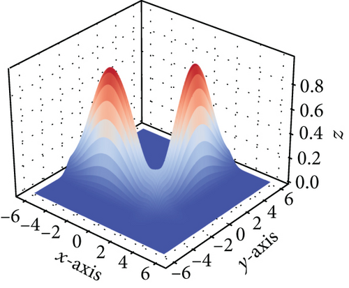
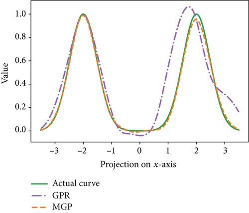
The first experiment is to test the regression performance of MGP compared with global GPR on a 2D toy function. The toy function consists of two bell-shaped local peaks, where one peak is sensitive on x-axis and the other one is on y-axis. The function is randomly sampled 100 times and the local experts are found by manually selecting the regions of each peak and then applying (11). Although the evaluation of the toy function is accurate, a small noise is assumed for the measurements to perform the update of the GPs. The kernel type used for the MGP is the Matérn kernel with v = 1.5, hence at least once differentiable. The regression result of MGP is taken to be the expected value of the posterior [14]:

(23)

It can be seen from Figure 2 that the MGP model trained using Algorithm 1 greatly outperforms the global GPR as the regression curve almost overlaps with the actual curve. Thanks to the gating function that assigns each model to the region where they excel, each peak is assigned to the corresponding local expert, leading to the outstanding regression performance. This recreates the results in Tresp [14] and indicates the success of the method for find local experts and the alternative gating network.

4.2. Test on Hyperparameter Tuning

The hyperparameter tuning problem in machine learning algorithms is a prime example of optimizing expensive black-box derivative-free functions. The hyperparameters of the machine learning models are specified prior to training and greatly affect the model performance. The training process can be very computationally expensive, and the performance of the trained model is usually noisy as randomness is typically involved during model training and testing.

Based on the successful implementation of the MGP model, Algorithm 2 for applying MGP in BayesOpt is tested on the hyperparameter tuning of four common machine learning algorithms. These algorithms are chosen for being highly tunable with large cross-validated average improvement after optimization [11]. The XGBoost is a boosting tree model, and its regularization is mainly controlled by the shrinkage factor and two penalty terms. The elastic net is a linear model that uses L₁ and L₂ penalties to reduce overfitting. The support vector machine (SVM) is a classifier using kernel trick, where its performance is determined by the regularization parameter and the kernel coefficient. The multilayer perceptron (MLP) is an artificial neural network, where the regularization term, the learning rate, and the hidden-layer sizes together contribute to its performance. The experiment is to test the efficiencies of the MGP-based BayesOpt in optimizing practical back-box derivative-free functions compared with the BayesOpt using GPR. The four algorithms above are trained on different datasets, and the configurations of their hyperparameters are optimized by the two types of Bayesian optimizers, respectively. The values of the current optima found by each optimizer are recorded in each iteration to compare the efficiency of optimization. Considering the MGP needs enough data to find the local experts, both optimizers start from a presampled dataset consisting of 5 random samplings followed by a few iterations of BayesOpt using GPR. The information for each tested model is given in Table 1.

Algorithm 2: MGP-based Bayesian optimization.

Input: pre-sampled data, the objective function, the term ϕ in the smoother,
the number of iterations N, minimum size of the clusters.
1 for iteration =1 to N: do
2 Standardize the data in the input space.
3 Filter out the data with values below the average.
4 Perform a density-based clustering for the rest data points.
5 Apply k-nearest neighbour classification on unselect data points.
6 Reject the clusters smaller than the minimum size.
7 Use Algorithm 1 to train the MGP.
8 /∗ The regions to optimize are the clusters found ∗/
9 Sample at the position that maximizes the acquisition function (22).
10 Add the sampled point to the data.
11 end for
Output: the value and the coordinates of the best sampled point.

Table 1. The settings for each tested model.

Model	Tuning dimension	Total presampling	Dataset
XGBoost	3	20	Housing [34]
Elastic net	2	10	Diabetes [35]
SVM	2	10	Wine type [36]
MLP	4	30	Artificial

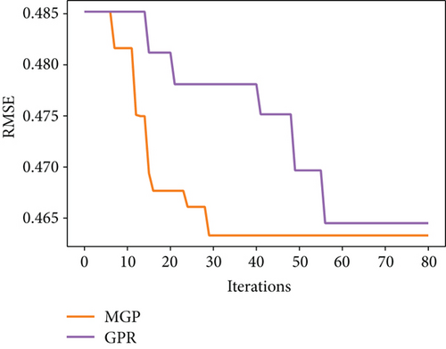
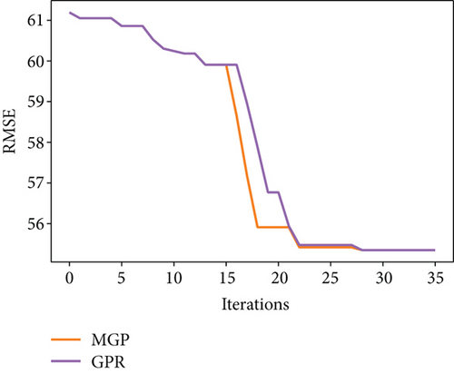
The comparison of tuning efficiency is presented in Figure 3. It can be seen that MGP model outperforms GPR in BayesOpt thanks to the more accurate modelling of the objective function. It is most significant in the test on XGBoost and MLP where the tuning dimension is relatively higher. This is reasonable as the higher dimension gives more space for tuning, while the other model converges too quickly to their optima even without the use of MGP. Such result marks the success of the clustering assisted method for finding the experts of the peaks. Interestingly, it is observed in the test on XGBoost and MLP that the number of GPs used in each optimizing iteration experienced an increase followed by a decrease. This corresponds to the design that lower peaks will be filtered out for lesser evaluation value.

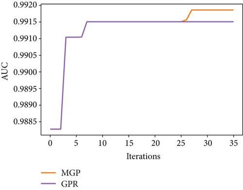
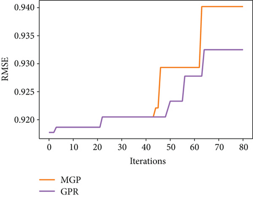
The presampling before applying MGP is important. It is observed that if the MGP-based BayesOpt is applied without a certain number of presamplings, its performance is not guaranteed to outperform the BayesOpt using GPR (see Figure 4). By examining the optimization processes, it is found that in situations where MGP fails to outperform the GPR, MGP stays in a local optimum (typically the first peak it finds) for longer iterations before moving to the global optimum, which is likely a cause of overfitting to the existing data. The use of MGP is based on the assumption that the behaviour of the objective function is well-represented by the sampled data. This assumption clearly breaks down when MGP is applied to optimize an objective function that is poorly explored. BayesOpt is a trade-off of exploitation and exploration, and MGP favours the former by increasing the complexity of the surrogate model, leading to a higher risk of overfitting and falling into local optima. MGP-based BayesOpt is definitely a good supplement to the GPR-based BayesOpt and may provide more accurate estimations in most cases. But the higher risk of overfitting implies it cannot be a complete replacement for GPR-based BayesOpt, especially when the input space is poorly sampled.

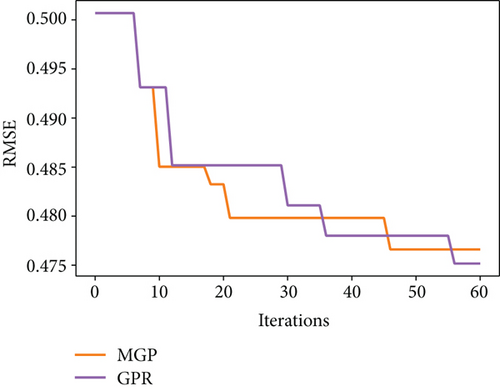
In practical optimization problems, it is advised to take enough samples using GPR before applying MGP to lower the risk of overfitting. One may also combine MGP and GPR together by switching back to GPR as the surrogate model every a few iterations of using MGP-based BayesOpt. This periodically decrease of model complexity makes a more robust optimization approach, having more accurate modelling while reducing the risk of overfitting. In our test where GPR is used every third iteration in the MGP-based BayesOpt, the phenomenon of being trapped in local optima is no longer observed and the combined method always outperforms the GPR-based BayesOpt.

5. Conclusion

This paper explained the motivations for replacing GPR by MGP in BayesOpt and provided a detailed introduction for implementing it. The method for finding the local experts, the alternative gating network, and the clustering-assisted method are proven to be successful by results in the experiment section. The MGP is a powerful candidate for achieving better regression performance than GPR. The BayesOpt based on it significantly outperforms the one using GPR especially for objective functions with larger input dimension. The only drawback of potential overfitting when optimizing with relatively few data can be addressed by more presampling or periodically switching back to GPR, making it an excellent supplement to the GPR-based BayesOpt. Despite the fact that MGP is computationally more expensive than a single GPR, it is still much faster to train than most machine learning algorithms and may significantly boost the efficiency of BayesOpt. Also, many steps in the EM can be trained in parallel, including the evaluation of the probability density for each data point. A fully optimized algorithm of MGP can undoubtedly speed up its implementation, providing a higher application value.

The methods are all explained with details, and the results are clearly illustrated and analysed to be satisfying. Hopefully, future works may be developed on improving the MGP or on finding more applications for it.

Conflicts of Interest

The authors declare that they have no conflicts of interest.

Authors’ Contributions

R.M. contributed the central idea and the major part of the software, carried out part of the experiment and analysis, revised the manuscript, and finalized this paper; C.C. provided the data, contributed part of the software, and completed the rest part of the experiment and analysis. The remaining authors equally contributed to refining the idea and designing the experiment. All authors discussed the results and wrote the initial draft of this paper.

Open Research

Data Availability

All data, models, and code generated or used during the study appear in the submitted article.

References

1 Booker A. J., DennisJ. E.Jr., Frank P. D., Serafini D. B., Torczon V., and Trosset M. W., A rigorous framework for optimization of expensive functions by surrogates, Structural Optimization. (1999) 17, no. 1, 1–13, https://doi.org/10.1007/BF01197708, 2-s2.0-0033077012.
10.1007/BF01197708
Web of Science® Google Scholar
2 Frazier P. I., A tutorial on Bayesian optimization, 2018, http://arxiv.org/abs/1807.02811.
Google Scholar
3 Regis R. G. and Shoemaker C. A., Parallel radial basis function methods for the global optimization of expensive functions, European Journal of Operational Research. (2007) 182, no. 2, 514–535, https://doi.org/10.1016/j.ejor.2006.08.040, 2-s2.0-34247494213.
10.1016/j.ejor.2006.08.040
Web of Science® Google Scholar
4 Jones D. R., Schonlau M., and Welch W. J., Efficient global optimization of expensive black-box functions, Journal of Global Optimization. (1998) 13, no. 4, 455–492, https://doi.org/10.1023/A:1008306431147, 2-s2.0-0000561424.
10.1023/A:1008306431147
Web of Science® Google Scholar
5 Mockus J., Bayesian Approach to Global Optimization: Theory and Applications, 2012, 37, Springer Science & Business Media.
Google Scholar
6 Lizotte D. J., Wang T., Bowling M. H., and Schuurmans D., Automatic gait optimization with Gaussian process regression, International Joint Conference on Artificial Intelligence. (2007) 7.
Google Scholar
7 Brochu E., Brochu T., and Freitas N. D., A Bayesian interactive optimization approach to procedural animation design, Proceedings of the 2010 ACM SIGGRAPH/Eurographics Symposium on Computer Animation, 2010, Madrid, Spain.
Google Scholar
8 Garnett R., Osborne M. A., and Roberts S. J., Bayesian optimization for sensor set selection, Proceedings of the 9th ACM/IEEE international conference on information processing in sensor networks, 2010, Stockholm Sweden, https://doi.org/10.1145/1791212.1791238, 2-s2.0-77954515653.
10.1145/1791212.1791238
Google Scholar
9 Snoek J., Larochelle H., and Adams R. P., Practical Bayesian optimization of machine learning algorithms, Advances in Neural Information Processing Systems. (2012) 25.
PubMed Google Scholar
10 Bergstra J., Yamins D., and Cox D. D., Hyperopt: a python library for optimizing the hyperparameters of machine learning algorithms, Proceedings of the 12th Python in science conference, 2013, Austin, Texas, United States, https://doi.org/10.25080/majora-8b375195-003.
10.25080/majora-8b375195-003
Google Scholar
11 Probst P., Boulesteix A.-L., and Bischl B., Tunability: importance of hyperparameters of machine learning algorithms, The Journal of Machine Learning Research. (2019) 20, no. 1, 1934–1965.
Web of Science® Google Scholar
12 Queipo N. V., Haftka R. T., Shyy W., Goel T., Vaidyanathan R., and Kevin Tucker P., Surrogate-based analysis and optimization, Progress in Aerospace Sciences. (2005) 41, no. 1, 1–28, https://doi.org/10.1016/j.paerosci.2005.02.001, 2-s2.0-17444368645.
10.1016/j.paerosci.2005.02.001
Web of Science® Google Scholar
13 Bergstra J., Bardenet R., Bengio Y., and Kégl B., Algorithms for hyper-parameter optimization, Advances in Neural Information Processing Systems. (2011) 24.
Google Scholar
14 Tresp V., Mixtures of Gaussian processes, Advances in Neural Information Processing Systems. (2000) 13.
Google Scholar
15 Jacobs R. A., Jordan M. I., Nowlan S. J., and Hinton G. E., Adaptive mixtures of local experts, Neural Computation. (1991) 3, no. 1, 79–87, https://doi.org/10.1162/neco.1991.3.1.79, 31141872.
10.1162/neco.1991.3.1.79
PubMed Web of Science® Google Scholar
16 Rasmussen C. and Ghahramani Z., Infinite mixtures of Gaussian process experts, Advances in Neural Information Processing Systems. (2001) 14.
Google Scholar
17 Prince S. J. D., Computer Vision: Models, Learning, and Inference, 2012, Cambridge University Press.
10.1017/CBO9780511996504
Google Scholar
18 Bishop C. M. and Nasrabadi N. M., Pattern Recognition and Machine Learning, 2006, 4, Springer, New York.
10.1007/978-0-387-45528-0
Google Scholar
19 Barber D., Bayesian Reasoning and Machine Learning, 2012, Cambridge University Press, https://doi.org/10.1017/CBO9780511804779.
10.1017/CBO9780511804779
Google Scholar
20 Williams C. K. and Rasmussen C. E., Gaussian Processes for Machine Learning, 2006, MIT press, Cambridge, MA.
Google Scholar
21 Sacks J., Welch W. J., Mitchell T. J., and Wynn H. P., The Design and Analysis of Computer Experiments, 2003, 1, Springer, New York, https://doi.org/10.1007/978-1-4757-3799-8.
Google Scholar
22 Eaton M. L., Multivariate Statistics: A Vector Space Approach, 1983, 512, John Wiley & Sons, Inc., New York, USA.
Google Scholar
23 Rossi R. J., Mathematical Statistics: An Introduction to Likelihood Based Inference, 2018, John Wiley & Sons.
10.1002/9781118771075
Google Scholar
24 Kushner H. J., A new method of locating the maximum point of an arbitrary multipeak curve in the presence of noise, Journal of Basic Engineering. (1964) 86, no. 1, 97–106, https://doi.org/10.1115/1.3653121, 2-s2.0-84998710865.
10.1115/1.3653121
Google Scholar
25 Močkus J., On Bayesian methods for seeking the extremum, Optimization Techniques IFIP Technical Conference, 1975, Springer, Berlin, Heidelberg, https://doi.org/10.1007/978-3-662-38527-2_55.
10.1007/978-3-662-38527-2_55
Google Scholar
26 Wu J., Chen X. Y., Zhang H., Xiong L. D., Lei H., and Deng S. H., Hyperparameter optimization for machine learning models based on Bayesian optimization, Journal of Electronic Science and Technology. (2019) 17, no. 1, 26–40, https://doi.org/10.11989/JEST.1674-862X.80904120, 2-s2.0-85064181166.
10.11989/JEST.1674-862X.80904120
Google Scholar
27 Clark C. E., The greatest of a finite set of random variables, Operations Research. (1961) 9, no. 2, 145–162, https://doi.org/10.1287/opre.9.2.145.
10.1287/opre.9.2.145
Web of Science® Google Scholar
28 Wu C. F. Jeff., On the convergence properties of the EM algorithm, The Annals of statistics. (1983) 11, 95–103.
10.1214/aos/1176346060
PubMed Web of Science® Google Scholar
29 Williams C. K. I. and Barber D., Bayesian classification with Gaussian processes, IEEE Transactions on Pattern Analysis and Machine Intelligence. (1998) 20, no. 12, 1342–1351, https://doi.org/10.1109/34.735807, 2-s2.0-0032289422.
10.1109/34.735807
Web of Science® Google Scholar
30 Stachniss C., Plagemann C., Lilienthal A. J., and Burgard W., Gas distribution modeling using sparse Gaussian process mixture models, International Conference on Robotics Science and Systems, Robotics: science and systems, 2008, June 2008, Zürich, Switzerland.
Google Scholar
31 Foster A., Li H., Maierhofer G., and Shearer M., An extension of standard latent Dirichlet allocation to multiple corpora, SIAM Undergraduate Research Online. (2016) 9, https://doi.org/10.1137/15s014599.
10.1137/15S014599
PubMed Google Scholar
32 Rasmussen C., The infinite Gaussian mixture model, Advances in Neural Information Processing Systems. (1999) 12.
Google Scholar
33 Gilks W. R. and Wild P., Adaptive rejection sampling for Gibbs sampling, Applied Statistics. (1992) 41, no. 2, 337–348, https://doi.org/10.2307/2347565.
10.2307/2347565
Web of Science® Google Scholar
34 The California housing dataset, Scikit-Learn Course, Scikit-Learn Developers, 2021, https://inria.github.io/scikit-learn-mooc/python_scripts/datasets_california_housing.html.
Google Scholar
35 Efron B., Hastie T., Johnstone I., and Tibshirani R., Least angle regression, The Annals of Statistics. (2004) 32, no. 2, 407–499, https://doi.org/10.1214/009053604000000067, 2-s2.0-3242708140.
10.1214/009053604000000067
Web of Science® Google Scholar
36 Cortez P., Cerdeira A., Almeida F., Matos T., and Reis J., Modeling wine preferences by data mining from physicochemical properties, Decision Support Systems. (2009) 47, no. 4, 547–553, https://doi.org/10.1016/j.dss.2009.05.016, 2-s2.0-72049084727.
10.1016/j.dss.2009.05.016
Web of Science® Google Scholar

Citing Literature

All articles

[Retracted] Mixture of Gaussian Processes Based on Bayesian Optimization

Retraction(s) for this article

Retracted: Mixture of Gaussian Processes Based on Bayesian Optimization

Abstract

1. Introduction