[Retracted] Advances in Hyperspectral Image Classification with a Bottleneck Attention Mechanism Based on 3D-FCNN Model and Imaging Spectrometer Sensor
Abstract
Deep learning approaches have significantly enhanced the classification accuracy of hyperspectral images (HSIs). However, the classification process still faces difficulties such as those posed by high data dimensions, large data volumes, and insufficient numbers of labeled samples. To enhance the classification accuracy and reduce the data dimensions and training needed for labeled samples, a 3D fully convolutional neural network (3D-FCNN) model was developed by including a bottleneck attention module. In such a model, the convolutional layer replaces the downsampling layer and the fully connected layer, and 3D full convolution is adopted to replace the commonly used 2D and 1D convolution operations. Thus, the loss of data in the dimensionality reduction process is effectively avoided. The bottleneck attention mechanism is introduced in the FCNN to reduce the redundancy of information and the number of labeled samples. The proposed method was compared to some advanced HSI classification approaches with deep networks, and five common HSI datasets were employed. The experiments showed that our network could achieve considerable classification accuracies by reducing the data dimensionality using a small number of labeled samples, thereby demonstrating its potential merits in the HSI classification process .
1. Introduction
The hyperspectral image (HSI) classification process is vital for the use of hyperspectral remote sensing data. The spectral resolution of HSI data ranges from visible light to short-wave infrared, with wavelengths reaching the order of nanometers. By exploiting the spectral characteristics of HSIs, one can effectively distinguish various objects, which has enabled the application of HSIs in a wide range of disciplines such as agriculture, early warning systems in disaster management, and national defense. Deep learning models for HSI classification are well developed. Many techniques, such as auto encoder [1], deep belief network [2], recurrent neural network [3], and convolutional neural network (CNN) models (e.g., the network described by Gu et al. [4]), are commonly used.
A convolution-related neural framework refers to a typical approach for deep learning [5–8] and HSI classification. It employs three types of models for the processing of a variety of characteristics by the CNN. The first type represents a 1D-CNN that uses only spectral data to extract the characteristics. This method requires a considerable number of training samples. The second type involves a spatial characteristics-based approach termed a 2D-CNN. Spatial characteristics are written by using a sparse representation method [9]; however, Makantasis et al. [10] developed a classification framework that uses particular scenes. The third type refers to the 3D-CNN approach that exploits spectral and spatial characteristics. It uses information on changes in local signals contained in spatial and spectral data without any pre- and postprocessing operations. The 3D convolution technique was initially employed to process videos, and it is currently used extensively in the HSI classification process [11–15]. Other methods are referred to as hybrid CNNs, and many such approaches have been developed for various uses [16, 17]. For instance, various hybrid approaches that adopt 1D-CNN and 2D-CNN were presented by Yang et al. [18] and Zhang et al. [17].
Previous studies on HSI classification based on deep learning have primarily discussed the building of deep networks to enhance accuracy. However, the number of training parameters was proportional to the complexity of the networks. For instance, approximately 360,000 training parameters were used in the classification network proposed by Zhong et al. [19]. Hamida et al. [20] proposed a 3D-1D hybrid CNN method that employs a maximum of 61,949 parameters. In the network proposed by Roy et al. [21], a 3D-2D hybrid CNN used 5,122,176 parameters. The adoption of such a high number of training parameters makes it difficult to train the network and is liable to result in overfitting. Other key issues also require attention, such as high data dimensionality, too few training-labeled samples, and spatial variability of spectral characteristics.
In this study, we present a 3D fully convolutional neural network (3D-FCNN) model with a bottleneck attention mechanism. The downsampling and fully connected layers are substituted by the convolutional layer. A 3D convolution operation is adopted to replace the commonly used 2D and 1D convolution operations, and a bottleneck attention mechanism is introduced to the FCNN to maintain end-to-end classification. A pooling layer is employed for dimension reduction and the final prediction of the classification result.
- (1)
The downsampling layer and the fully connected layer are substituted by convolutional layers, and multiple datasets are adopted to separately alter the model and network depth. The developed network shows improved performance in comparison with several advanced HSI classification approaches with deep networks
- (2)
Network parameters are significantly reduced without adopting the fully connected layer
- (3)
A bottleneck attention mechanism is added to determine the latest classification accuracy in a dataset that includes limited training data. Moreover, the time consumed by the developed network is significantly decreased
The rest of the paper is organized as follows: In Section 2, literature related to CNN is presented; in Section 3, the proposed 3D-FCNN structure following the bottleneck attention mechanism is elucidated; in Section 4, the experimental results are presented and analyzed; in Section 5, conclusions are drawn, and the direction of future research is highlighted.
2. Convolutional Neural Network (CNN)
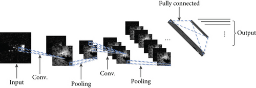
The CNN exploits feature extraction and a weight sharing mechanism to decrease the number of network training parameters required; its structure is illustrated in Figure 1. The working mechanism involves inputting image data and passing it to the convolutional layer for image feature extraction. The downsampling layer reduces the features of the current results. After several cycles of alternating learning of the convolution and downsampling layers, the data are acquired via the rectified linear unit (ReLU) activation function with high-level abstract characteristics. The acquired abstract characteristics are introduced into a 1D vector, passed to the fully connected layer, subsequently passed to the learning of several fully connected layers, and finally outputted to the classifier to complete the entire classification of the image.
2.1. Convolutional Layer

2.2. Downsampling Layer
2.3. Fully Connected Layer
2.4. Network Training
The training process of the CNN covers two stages, i.e., forward propagation with low-level propagation and high-level propagation and back propagation with high-level propagation and low-level propagation. Figure 3 presents the entire CNN training process.
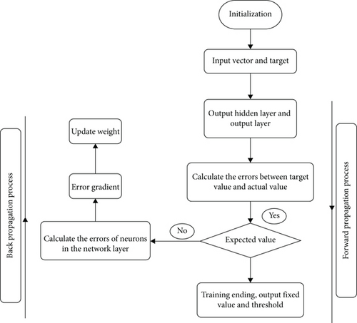
The input weight parameters are first initialized to avoid gradient propagation problems, reduced training speeds, and consumption of training time. Then, the actual output is obtained after a series of forwarding propagations (e.g., a convolutional layer, downsampling layer, and fully connected layer). The error between the actual output value and the target value is calculated. If the error generated is not consistent with the expected value, the error is retransmitted to the network for training, and the backpropagation sequentially calculates the fully connected, downsampling, and convolutional layers. The weight is updated following the calculated error value, and the mentioned steps are repeated until the error is less than the expected value; then, the training is terminated.
3. 3D-FCNN Structure with a Bottleneck Attention Mechanism
In this section, a new 3D fully convolutional neural network model will be presented to overcome difficulties in the process of hyperspectral images classification. In this model, the downsampling layer and the fully connected layer are replaced with a 3D-CNN, and a bottleneck attention mechanism is embedded. The structure of the elementary block of the developed model is first illustrated, and then the method by which the block extracts and fuses the characteristics is elucidated. Lastly, the bottleneck attention mechanism architecture is detailed.
3.1. 3D-FCNN Module
- (1)
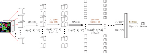
Extraction of training samples. The N × N × L image cube is extracted from the HSI with the input size of H × W × L, where N × N denotes the size of the neighborhood space (window size) and L represents the number of spectral bands
- (2)
Spectral-spatial feature extraction based on 3D-FCNN. The model in the present study substitutes all downsampling layers with convolutional layers with a step size of S
- (3)
Classification based on spatial-spectral features. The characteristics of the last layer, i.e., the 1 × 1 × 1 × N tensor, are input into the SoftMax classifier to acquire the final classification result
3.2. Bottleneck Attention Mechanism Module
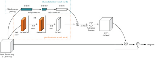
The bottleneck attention module (BAM) [20, 24] is embedded based on the 3D-FCNN classification network. The BAM extracts vital information from the spectral and spatial dimensions of the HSI through the channel and spatial attention branches, respectively, and exploits the characteristics separately without any feature engineering. The end-to-end characteristics are maintained, and the problem of information redundancy is effectively solved.
3.2.1. Channel Attention Branch
3.2.2. Spatial Attention Branch
3.2.3. Merging of the Two Attention Branches
After the channel MC(F) and the spatial MS(F) attention branches are obtained, these are merged to generate the final 3D attention feature map M(F). The summation maps of the attention feature maps of each branch to the size of R are obtained and are impacted by the different shapes of the attention feature maps generated by the two branches. In a range of combination methods (e.g., summation, multiplication, or maximum value operations), the corresponding elements act as the operation method. After the summation, the swish function is adopted to activate the final 3D attention feature mapping M(F). The generated 3D attention feature map M(F) is subsequently introduced to the original input feature map F to multiply the corresponding elements in it and generate the redefined feature map F′ as expressed in the formula, i.e., to generate the BAM-processed feature map.
3.2.4. Swish Activation Function
The common activation function in deep learning is the ReLU activation function characterized by a lower bound, no upper bound, and smoothness. Swish has a lower bound and no upper bound similar to ReLU, whereas the nonmonotonicity of swish is inconsistent with other common activation functions. Moreover, swish exhibits both first-order derivative and second-order derivative smoothness.
3.2.5. 3D-FCNN Model with BAM
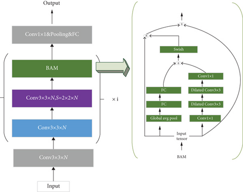
The major convolution part of the model network covers a convolutional layer and a convolutional layer with a step length of S. The N × N × L image cube of an HSI with the size H × W × L is extracted as a sample input of the network. N × N denotes the size of the neighborhood space (window size), and L represents the spectral band number. The type of the center pixel of the cube acts as the target label. After inputting the data samples, it first passes through a 3 × 3 × L convolutional layer. The second refers to a small-structure network covering a convolutional layer, a convolutional layer with a step size of S, and an added BAM. The number of times the small network module is superimposed is i. The last attention mechanism feature map generated undergoes a 1 × 1 convolution, global pooling, and fully connected operation. Then, the SoftMax function is adopted to output the final classification. The model is illustrated in Figure 6.
4. Results and Discussion
To evaluate the accuracy and efficiency of the developed model, experimental processes with respect to five datasets were created for comparison and verification with other approaches. For accurate measurements of each approach, quantitative metrics of Kappa (K), average accuracy (AA), and overall accuracy (OA) were employed. Here, OA denotes the rate of true classification of whole pixels, AA refers to the average accuracy characteristic of all types, and Kappa indicates the consistency characteristic of ground truth with the classification result. The higher these metrics are, the more effective the classification result is.
4.1. Introduction to the Dataset
- (i)
Indian Pines (IP): generated by the airborne visible infrared imaging spectrometer (AVIRIS) sensor in north-western Indiana, the IP dataset covers 200 spectral bands exhibiting a wavelength scope of 0.4 to 2.5 μm and 16 land cover classes. IP covers 145 × 145 pixels and exhibits a resolution of 20 m/pixel
- (ii)
Pavia University (UP) and Pavia Center (PC): collected by the reflective optics imaging spectrometer (ROSIS-3) sensor at the University of Pavia, northern Italy, the UP dataset covers 103 spectral bands exhibiting a wavelength scope of 0.43 to 0.86 μm and 9 land cover classes. UP encompasses 610 × 340 pixels and exhibits a resolution of 1.3 m/pixel. The PC reaches 1096 × 715 pixels
- (iii)
Salinas Valley (SV): collected by the AVIRIS sensor from Salinas Valley, CA, USA, the SV dataset covers 204 spectral bands exhibiting a wavelength scope of 0.4 to 2.5 μm and 16 land cover classes. SV encompasses 512 × 217 pixels and exhibits a resolution of 3.7 m/pixel
- (iv)
Botswana (BS): captured by the NASA EO-1 satellite over the Okavango Delta, Botswana, the BS dataset covers 145 spectral bands exhibiting a wavelength scope of 0.4 to 2.5 μm and 14 land cover classes. BS encompasses 1476 × 256 pixels and exhibits a resolution of 30 m/pixel
Deep learning algorithms are data driven and rely on large numbers of labeled training samples. As more labeled data are fed into the training, the accuracy improves. However, more data for training implies increased time consumption and higher computation complexity. The five datasets used by the 3D-FCNN are the same as those used by the other networks discussed, and we set the parameters based on experience. For the IP dataset, 50% of the samples were selected for training, and 5% were randomly selected for verification. Since the samples were sufficient for UP, PC, BS, and SV, only 10% of the samples were used for training, and the remaining 90% were used as test data. Of the 10% of samples used for training, 50% (5% of the total) were randomly selected. Accordingly, different models and different network depths were compared under identical data conditions. Notably, in the absence of training samples, the model based on the BAM was capable of maintaining excellent performance. Thus, in the experiment, the sizes of the training and verification samples were set to the minimum level. The IP and SV datasets were employed for the experimental processes. Owing to the uneven distribution of the number of types in the IP dataset, the ratio of training-set : test-set was maintained at 1 : 1. As the number of labeled samples in the SV dataset is identical among different types, the ratio of training-set : test-set was maintained at 1 : 9.
4.2. Experimental Settings
To assess the effectiveness of the model, deep learning-based classifiers (SVM, 1D-NN, 1D-CNN, 2D-CNN, and 3D-CNN) were utilized to compare with our proposed framework. Under identical conditions, comparisons of the generalization ability and nonlinear expression ability at different network depths were conducted. The BAM added with the parameter r = 5 was employed in the CNN model. Two other methods, SE-Net [27] (squeeze-and-excitation (SE)) and frequency band weighted module [28] (band attention module, (BandAM)), were also employed. The classification results were compared. To ensure the validity of the experiment, the same depth was maintained for all involved models, and 10 experiments were carried out to eliminate randomness.
The patch size of each classifier was set as specified in the corresponding original paper. To compare the classification performances, all experiments were performed on the same platform with 32 GB of memory and an NVIDIA GeForce RTX 2080 Ti GPU. All classifiers based on deep learning were implemented by adopting PyTorch, TensorFlow, and Keras libraries.
4.3. Experimental Results
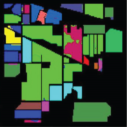
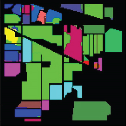
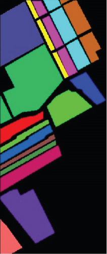
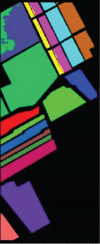
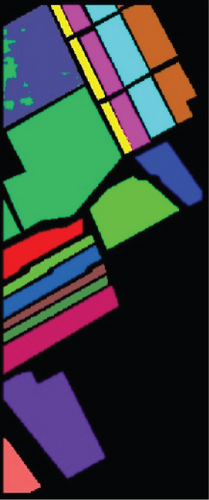
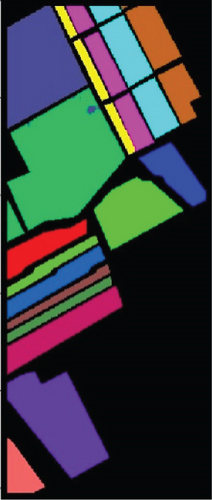
For SVM, 1D-NN, 1D-CNN, 2D-CNN, and 3D-CNN, the same architecture and parameter settings as in the present study were used. For those settings that are not explicitly given in the present study, we used commonly used values in the HSI classification (for example, the merge span is 2). Detailed analysis results are presented in Tables 1–3. The classification effect diagrams of various datasets under different models are presented in Figure 7 for IP, Figure 8 for PC, Figure 9 for UP, Figure 10 for BS, and Figure 11 for SV.
| Class | SVM | 1D-NN | 1D-CNN | 2D-CNN | 3D-CNN | 3D-FCNN |
|---|---|---|---|---|---|---|
| IP | 73.03 | 83.89 | 87.68 | 96.69 | 98.66 | 99.32 |
| PC | 94.70 | 96.18 | 96.21 | 97.23 | 98.57 | 98.82 |
| UP | 90.39 | 91.48 | 91.97 | 96.04 | 97.34 | 99.07 |
| BS | 80.63 | 81.05 | 89.81 | 90.60 | 90.97 | 97.23 |
| SV | 90.36 | 93.38 | 95.87 | 96.66 | 96.90 | 98.59 |
| Class | SVM | 1D-NN | 1D-CNN | 2D-CNN | 3D-CNN | 3D-FCNN |
|---|---|---|---|---|---|---|
| IP | 81.27 | 84.77 | 86.20 | 95.27 | 99.07 | 99.25 |
| PC | 98.22 | 98.74 | 98.87 | 98.90 | 98.93 | 99.63 |
| UP | 91.54 | 92.60 | 93.44 | 94.07 | 95.72 | 99.60 |
| BS | 77.83 | 80.44 | 88.96 | 89.72 | 90.69 | 97.02 |
| SV | 87.01 | 89.09 | 92.37 | 93.00 | 94.40 | 96.97 |
| Class | SVM | 1D-NN | 1D-CNN | 2D-CNN | 3D-CNN | 3D-FCNN |
|---|---|---|---|---|---|---|
| IP | 78.61 | 64.39 | 84.21 | 94.64 | 98.93 | 99.51 |
| PC | 97.50 | 98.22 | 98.40 | 98.51 | 98.48 | 99.47 |
| UP | 89.07 | 90.17 | 91.52 | 92.25 | 94.40 | 99.47 |
| BS | 75.14 | 78.80 | 88.04 | 88.26 | 89.91 | 96.07 |
| SV | 85.48 | 87.86 | 91.49 | 90.22 | 93.77 | 96.62 |
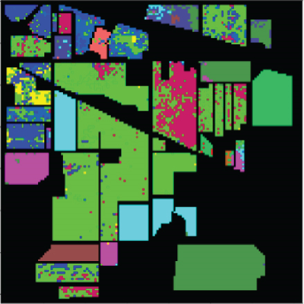
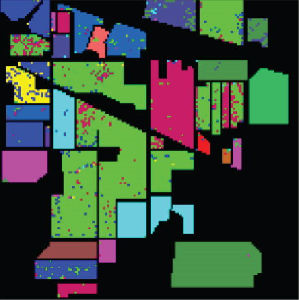
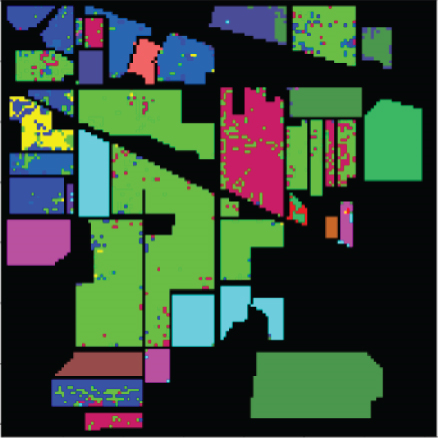
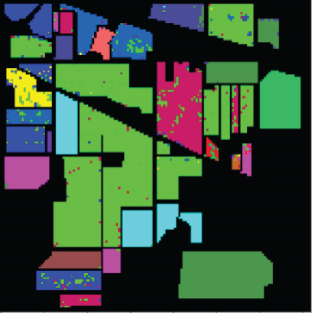
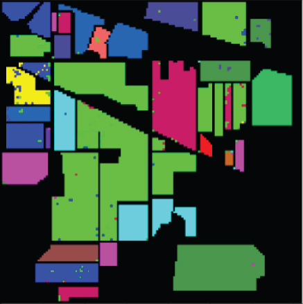
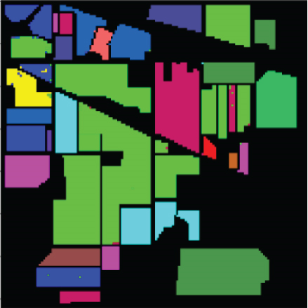
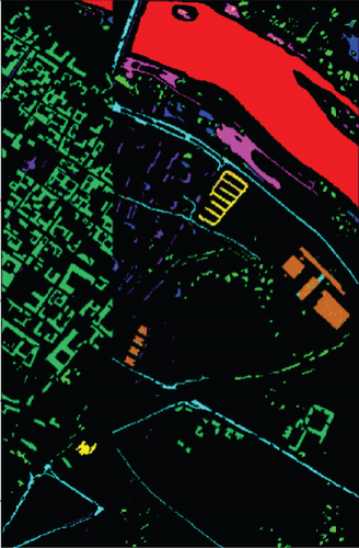
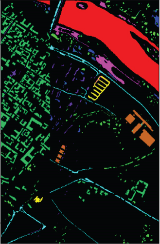
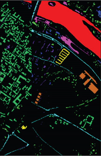
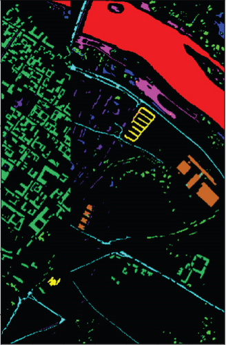
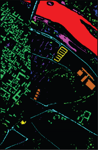
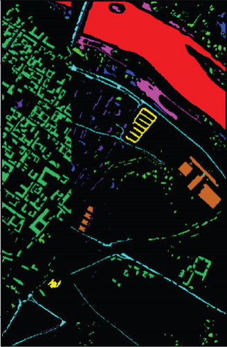


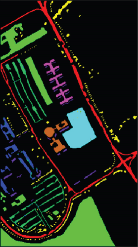

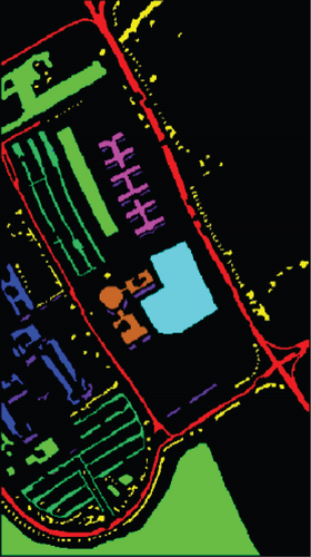


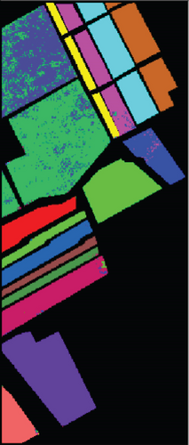
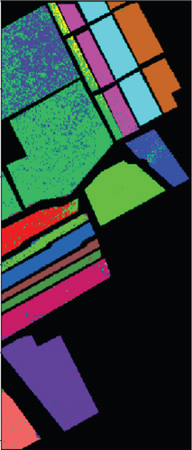
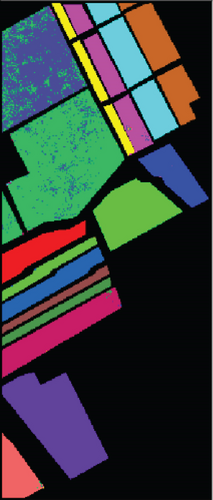
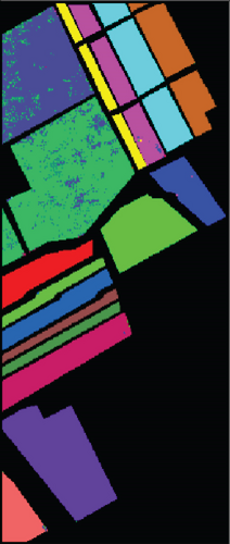


Our 3D-FCNN network replaces the downsampling layer and the fully connected layer with a CNN, which reduces the network training parameters, consumes less training time under identical conditions, and has a higher convergence speed, thus showing better overall performance. Furthermore, the model developed in the present study has the best classification performance with a classification accuracy of 99.63% and minimum classification error based on the three evaluation criteria. Adopting CNNs to replace the downsampling layer and the fully connected layer is suggested as a potentially feasible approach for training the deep network.
The number of network model layers (depth) is another critical parameter that should be considered. In the case of a fixed input data cube size, different network layers are employed for multiple datasets to further demonstrate the impact of the depth parameter on the classification results. The experimental processes were performed on the datasets and compared with the 3D-CNN model under identical conditions. The number of layers was 3, 5, 7, and 9. Table 4 shows the comparative results. Figure 12 presents the performances of the two models on the respective datasets at various depths.
| Model | Dataset | 3 | 5 | 7 | 9 | 11 |
|---|---|---|---|---|---|---|
| 3D-CNN | IP | 87.78 | 99.07 | 77.69 | 75.76 | 73.04 |
| PC | 95.62 | 98.93 | 97.03 | 96.22 | 95.00 | |
| UP | 93.79 | 94.01 | 95.72 | 95.11 | 94.25 | |
| BS | 88.04 | 90.69 | 88.96 | 87.13 | 85.64 | |
| SV | 93.08 | 94.40 | 94.05 | 93.33 | 92.57 | |
| 3D-FCNN | IP | 89.60 | 99.25 | 98.51 | 96.35 | 95.63 |
| PC | 99.33 | 99.63 | 99.68 | 98.72 | 97.77 | |
| UP | 94.80 | 98.25 | 98.49 | 98.55 | 98.41 | |
| BS | 88.44 | 96.13 | 97.02 | 95.45 | 94.28 | |
| SV | 93.76 | 96.38 | 96.97 | 95.87 | 95.44 |
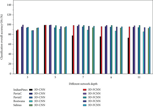
The results show that, regardless of depth, the model developed in this study outperforms the 3D-CNN model. The 3D-FCNN model developed in the present study has better performance generalization and nonlinear expression abilities under identical conditions.
Figure 12 shows the results of different network depths. Overall, the network is better with increasing depth. Furthermore, increasing depth facilitates extraction and classification using more advanced functions. However, the results of our model are not proportional to the depth of the network, as the architecture of the developed model balances performance and cost by selecting the optimal network layer.
An optimized FCNN acts as the basic network. The network does not perform any operations and directly performs classification. The other three methods use different band weighted inputs, including the BandAM module, SE module, and the BAM proposed in the present study. Tables 5 and 6 present the specific analysis and comparison. The classification effect diagrams of various datasets under different modules (Figure 13 for IP and Figure 14 for SV) are illustrated.
| Class | 3D-FCNN | SE+3D-FCNN | BandAM+3D-FCNN | BAM+3D-FCNN |
|---|---|---|---|---|
| 1 | 53.33 | 100 | 52.27 | 100 |
| 2 | 82.74 | 98.10 | 99.19 | 95.49 |
| 3 | 59.61 | 98.04 | 88.09 | 98.66 |
| 4 | 64.68 | 100 | 80.89 | 97.65 |
| 5 | 67.78 | 27.93 | 94.12 | 97.47 |
| 6 | 99.03 | 99.11 | 98.70 | 98.93 |
| 7 | 0 | 96.15 | 74.07 | 100 |
| 8 | 94.29 | 100 | 100 | 100 |
| 9 | 0 | 88.89 | 73.68 | 94.44 |
| 10 | 94.24 | 94.27 | 79.74 | 97.60 |
| 11 | 90.09 | 99.25 | 97.13 | 99.91 |
| 12 | 67.12 | 95.79 | 82.77 | 98.88 |
| 13 | 99.01 | 100 | 91.79 | 100 |
| 14 | 97.60 | 99.05 | 99.50 | 99.03 |
| 15 | 89.79 | 97.45 | 92.64 | 99.42 |
| 16 | 65.22 | 100 | 100 | 98.81 |
| OA (%) | 82.29 | 93.01 | 93.66 | 98.54 |
| AA (%) | 71.00 | 93.36 | 88.13 | 98.51 |
| Kappa | 79.64 | 91.98 | 92.75 | 98.33 |
| Class | 3D-FCNN | SE+3D-FCNN | BandAM+3D-FCNN | BAM+3D-FCNN |
|---|---|---|---|---|
| 1 | 100 | 98.99 | 100 | 100 |
| 2 | 100 | 100 | 100 | 100 |
| 3 | 100 | 99.90 | 100 | 100 |
| 4 | 100 | 100 | 99.76 | 98.49 |
| 5 | 94.19 | 95.44 | 99.75 | 99.96 |
| 6 | 100 | 98.55 | 100 | 100 |
| 7 | 100 | 100 | 100 | 99.76 |
| 8 | 99.93 | 97.65 | 100 | 99.08 |
| 9 | 100 | 100 | 100 | 100 |
| 10 | 99.97 | 99.32 | 100 | 100 |
| 11 | 100 | 99.62 | 100 | 100 |
| 12 | 100 | 96.59 | 100 | 99.78 |
| 13 | 100 | 98.90 | 100 | 100 |
| 14 | 99.90 | 99.72 | 99.79 | 100 |
| 15 | 79.80 | 93.39 | 91.48 | 99.96 |
| 16 | 99.94 | 99.94 | 100 | 100 |
| OA (%) | 96.88 | 98.05 | 98.83 | 99.73 |
| AA (%) | 98.27 | 98.59 | 99.39 | 99.81 |
| Kappa | 96.52 | 97.83 | 98.70 | 99.70 |




In this study, we explored a novel and effective 3D-FCNN for HSI classification. On this basis, we embedded a module for the extraction of spectral and spatial features. Compared to the latest network, the most significant advantage of the proposed network is that it requires only a small number of network parameters to achieve considerable classification accuracy, in which an end-to-end classification mechanism is maintained. The proposed network uses various training strategies to help it converge better and faster without causing a computational burden.
5. Conclusions
- (1)
Deep networks that adopt spectral and spatial characteristics achieve significantly higher classification accuracy than deep networks that adopt only spectral characteristics. The results prove that the BAM is beneficial to HSI classification
- (2)
Deep learning performs well in several remote sensing fields. However, the trend to make the network more complex and deeper adds several parameters to the training process. With the inclusion of more parameters, the model can exhibit better classification capabilities. The results of the present study showed that this attempt has successfully reduced the network parameters and the loss of data information. That is, the developed method successfully replaces the downsampling layer and the fully connected layer with a convolutional layer. Furthermore, the experimental results show that the proposed network exhibits a high generalization ability and classification performance irrespective of its depth
- (1)
Application of the developed framework to HSIs in specific areas, such as forest resources observation and agricultural production management, other than the open-source datasets considered here
- (2)
The methods applied in the present study are all supervised. Semisupervised or unsupervised methods can be adopted using the considered limited data and achieve relatively higher performance with less labeled data
- (3)
The reduction in the training time poses an attractive challenge and needs to be addressed
Conflicts of Interest
The authors declare no conflict of interest.
Acknowledgments
This research was funded by the National Natural Science Foundation of China (grant number: 61501210) and the Department of Education of Jiangxi Province (grant number: GJJ211410).
Open Research
Data Availability
All code will be made available on request to the correspondent author’s email with appropriate justification.


