Landslide susceptibility mapping is considered a useful tool for planning, disaster management, and natural hazard mitigation of a region. Although there are different methods for predicting landslide susceptibility, the bivariate statistical analysis method is considered to be simple and popular. In this study, the main aim is to evaluate the performance of Shannon entropy (SE) and weights of evidence (WOE) statistical models in landslide susceptibility mapping of Pithoragarh district of Uttarakhand state, India. For this purpose, ten landslide affecting factors, namely, slope degree, aspect, curvature, elevation, land cover, slope forming materials, geomorphology (landforms), distance to rivers, distance to roads, and overburden depth were used for the development of landslide susceptibility maps using the SE and WOE methods. Data extracted from the Google Earth images, Aster Digital Elevation Model, and Geological Survey of India report were used for the construction and evaluation of landslide susceptibility models and maps. The landslide data of 91 locations were randomly divided into two parts in the ratio of 70 : 30 using GIS software that is 70% data was used for training the models and 30% data was used for testing and validating the models. Performance of the applied models was evaluated using area under the AUC (area under the curve) ROC (receiver operating characteristics) curve. Results indicated that the WOE model is having better accuracy (AUC_WOE = 68.75%) than the SE model (AUC_SE = 52.17%) in the development of landslide susceptibility maps. Hence, WOE model can be used for the development of accurate landslide susceptibility maps which can provide useful information to decision maker and policy planner in better development of landslide prone areas.

1. Introduction

Landslides are one of the most dangerous and threatening natural disasters for various communities around the world causing huge loss of life, economy, and infrastructures [1]. Landslides are downward gravitational movement of rocks and soil [1]. Landslides destabilizes the ground stability and can enhance soil formation in the area [2, 3]. It can also affect sustainable development goals of the United Nations and the land degradation neutrality challenge [4]. Factors which affect landslides include geology, topography, land use pattern, rainfall and other geo-environmental factors. Out of these, geology is one of the most important factors in the occurrence of landslides [5]. Recently, climate change effects have increased landslides events all over the world [6, 7].

Landslide susceptibility map is an important tool in the landslide management of the area [8, 9]. These maps help in the reduction of landslide risk on human life, infrastructures, communication and in proper planning of land use [10]. Landslide susceptibility refers to the probability of a landslide which may occur in an area in future, based on the past events under similar conditions [11]. There are various methods of generation of landslide susceptibility maps such as statistical methods, in conjunction with Geographical Information System (GIS) and remote sensing techniques [12–16]. Some of these methods include multivariate regression, likelihood ratio, information value, logistic regression, and binary logistic regression [17–22]. Other algorithms which have acceptable accuracy in landslide susceptibility mapping are discriminant analysis, analytic hierarchy processes, weights of evidence, weighted linear combinations, evidential belief functions, and generalized additive models [8, 23–25]. Shannon’s entropy is another important bivariate algorithm used to analyze landslide susceptibility [26]. Other statistical methods for landslide susceptibility mapping (zoning) are probabilistic models, certainty factors, information values, modified bayesian estimation, weighting variables, weighted linear combinations of instability variables, landside nominal risk variables [27–30], spatial multicriteria evaluation, index of entropy, and Dempster–Shafer models [31–36].

In recent years, researchers have widely used machine learning (ML) algorithms in the natural hazard studies including landslide susceptibility modeling such as support vector machine, multivariate adaptive regression spline, boosted regression, classification and regression trees, Naïve Bayes, quadratic discriminant analysis, artificial neural networks, maximum entropy, random forest, and generalized linear model [37–44]. However, simple statistical methods/models are also being applied in the landslide studies to understand relationship between affecting variables/factors and occurrence of landslides. In this study, we have used Shannon entropy (SE) and weights of evidence (WOE) popular statistical models for the development of landslide susceptibility maps of Pithoragadh district of Uttarakhand State, India, which is one of the prominent landslide prone areas in the Himalayan region. For the evaluation of statistical models, we have used ten landslide affecting factors: slope degree, aspect, curvature, and elevation, land cover, slope forming materials (SFM), geomorphology (landforms), distance to rivers, distance to roads, and overburden depth. Rainfall is generally acted as a triggering factor in the occurrence of landslides in the Himalayan region, therefore this factor has not been considered separately in the model studies. Data for the use in statistical models were extracted from the Geological Survey of India (GSI) report (https://www.gsi.gov.in/webcenter/portal), Google Earth images, and Aster Digital Elevation Model (DEM). Performance of the models was evaluated using area under the receiver operating characteristic (ROC) curve method. GIS software was used for data integration and visualization.

2. Study Area

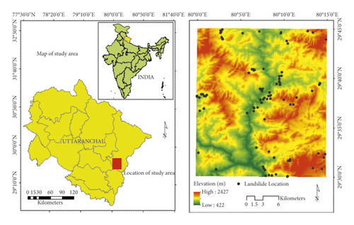
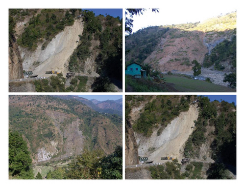
Topography of the Pithoragdh district is rugged mountainous mark by steep hills and deep valleys (Figure 1). General elevation in the study area ranges from 1500 m (in south) to 2500 m (in north) above mean sea level. Sarju and Ramganga Rivers are prominent rivers traversing the area. Google Earth images and GSI map shows that landslides are very prominent along the excavated slopes of road sections and on steep sides of river valleys such as Bansura-Rameshwar Ghat Road and along Sarju river (Figure 2). Geologically, rocks of almora crystalline (granitoids) and garhwal group (shale, slate, phyllite, quartzite, dolomite, limestone, magnesite, occasional calc slate, and metavolcanics) separated by thrust fault are present in this area (https://www.gsi.gov.in/webcenter/portal). The area is affected by tectonic activities indicated by folded and faulted rocks. Quaternary sediments are present in river valleys, on hill slopes and as glacial deposits.

Details are in the caption following the image — Open in figure viewer PowerPoint

Climate of the area varies from the moist lower elevation to cold temperate and rain shadow (higher elevation). There are four main seasons in the district: winter (December to mid-March), summer (mid-March to mid June), and rainy (mid-June to mid-September), transitional that is season of retreating monsoon (mid-September to November). Temperature varies from subzero in winter (at higher elevation) to 40 to 45 degree in summer (at lower elevation).

Most part of the Pithoragarh district is a highly vulnerable to landslides, hence selected as study area. The area is tectonically disturbed and geologically dissected by faults, shears, and joints and thus affected by more landslides in the event of heavy rains or due to excavation of roads and other infrastructure projects. Numerous landslides occurrences have been recorded in the past and present necessitating systematic studies for proper monitoring and prevention of landslides for the proper development of the area. The most catastrophic landslide caused by unprecedented rains, killing 221 people occurred in the early morning of August 18, 1998, in Malpa in Pithoragarh district [45].

3. Materials and Methods

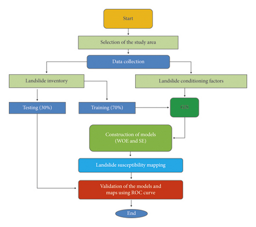
Methodological flowchart of this study is presented in Figure 3 which is self-explanatory:

3.1. Shannon Entropy

Entropy is one of the management approaches that has been used to deal with the disorder, instability, turbulence, and uncertainty in a system and has shown the amount of uncertainty in a continuous probability distribution [46]. In fact, the entropy is a concept that estimates dispersion and disorder in natural phenomena. This concept, which is widely used in the science of thermodynamics, has spread to other sciences today [47]. The theory of entropy was first quantified by Shannon [46]. In Shannon entropy (SE) [46], the variables with the maximum impact on the occurrence of an event are determined [48]. To use this model, a decision matrix must first be created. The decision matrix contains information that entropy can be used to evaluate, and by calculating the entropy matrix and the total weight of the ten landslide factors used in this study. The following equations were used to plot the map using the SE model [27, 48]:

(1)

Where P_ij is the landslide density in each class, (P_ij) is the probability of landslides in each factor and its related classes, H_j and (H_j) are entropy values and maximum entropy, I_j is the information coefficient, W_ij is the final weight of each factor. After determining the final weight of each factor and multiplying it in the mentioned factor classes, i.e., the P_ij values of each factor and its classes based on dividing the number of landslides by the number of pixels of the factor classes, finally the weight maps were added together. Final landslide maps were prepared and the more sensitive floors took on more weight [49].

3.2. Weights of Evidence

Weights of evidence (WOE) or conditional probability method was first developed to identify and explore mineral deposits [50]. Conditional probability analysis is a valuable tool in determining risk zoning especially, when appropriate factors and good knowledge of the variables affecting the landslide are available. This theory is a data-driven method that is known as one of the models of Bayesian theory in the form of linear algorithm and uses the previous (unconditional) and posterior (conditional) probabilities [51]. This method (WOE) is used when sufficient data is considered to estimate the relative importance of the issues substantiated through statistics. For this purpose, first, the probabilistic weights of each factor and its related classifications are calculated using the following relationships [52].

(2)

Then, the following equations were calculated and the final weight for each factor was used to zoning the landslide susceptibility.

(3)

where N_pix1 is number of sliding pixels in a class, N_pix2 (total number of sliding pixels in a map)-(number of sliding pixels in a class), N_pix3 (number of sliding pixels in a class)-(number of sliding pixels in a class), N_pix4: (total number of pixels in a map)-(total number of sliding pixels in a map)-(number of pixels in a class).

(4)

where C is the difference of positive and negative weights, W_final: standardized final weight and S_c: standard deviation, which is equal to the root of the variance of each of the positive and negative weights [53].

3.3. Evaluation Method Using Receiver Operating Characteristic (ROC) Curve

Area under the receiver operating characteristic (ROC) curve is a well-known method for evaluating and comparing the accuracy of algorithms used to prepare landslide susceptibility maps [54]. Validation and accuracy evaluation of bivariate statistical models were done on 30% testing or validation data which was randomly selected from the landslide occurrence points during the spatial modeling process [55]. The ROC curve is a two dimension graph that has landslide susceptibility as real (true) positive rate on Y-axis (sensitivity) and false positive rate on X-axis (1-specificity) with different cut-off, which was used for numerical appraisal of landslide susceptibility of the prediction maps [56]. Area under ROC curve, detects the precision of the models [57]. The AUC value varies between 0.5 and 1 [57]. The model with excellent accuracy in predicting landslide susceptibility has a value of AUC = 1 and the weak (non-instructive) model has an AUC of 0.5. As well as, the area below the ROC curve represents the predicted value of the system by describing its ability to accurately estimate the occurrence or occurrence of landslide events and the absence of landslides [57].

3.4. Data Used

3.4.1. Landslide Inventory

One of the most important part of landslide susceptibility mapping and zoning is to prepare landslide inventory showing geospatial distribution of landslide events in a map [58]. For the development of models, landslide polygon data represented by points on the map was randomly divided into two parts in the ratio of 70:30 as training dataset and validation data set, respectively [59–61]. The training data set (70%) was used for landslide susceptibility mapping/zoning and remaining 30% testing dataset (validation) for the validation and accuracy evaluation of the models used.

In this study, the inventory of past 91 landslide events was prepared based on the available past record of Geological Survey of India (https://www.gsi.gov.in/webcenter/portal) which showed a predominant percentage of debris slip (61 cases) and less number of rock slips (17 cases) and slight falls/flips (3 cases). Furthermore, there were only 6 cases of deep damage (5 debris slip, 1 rock slip) while the rest were shallow damage. In addition, several recent landslides were included in the inventory by interpreting of Google Earth images (Table 1, Figures 1 and 2). Most of the landslides in the area occurred during heavy rainfall especially along roads and on steep hill/valley slopes covered by loose soil and rock debris and in the areas where groundmass/rock mass is weathered and dissected by structural discontinuities.

1. Data used in this study.

No	Data	Source	Resolution
1	Landslide inventory	Geological Survey of India report (https://www.gsi.gov.in/webcenter/portal) google earth imanges	1 : 50,000
2	Digital elevation model (DEM)	USGS (https://earthexplorer.usgs.gov)	30m
3	Land cover	Geological Survey of India report (https://www.gsi.gov.in/webcenter/portal)	1 : 50,000
4	Landforms (geomorphology)	Geological Survey of India report (https://www.gsi.gov.in/webcenter/portal)	1 : 50,000
5	Roads	Google Earth images	1 : 50,000
4	Rivers	DEM (https://earthexplorer.usgs.gov)	30m
5	Slope forming materials (SFM)	Geological Survey of India report (https://www.gsi.gov.in/webcenter/portal)	1 : 50,000
6	Overburden depth	Geological Survey of India report (https://www.gsi.gov.in/webcenter/portal)	1 : 50,000

3.4.2. Factors Affecting Landslides

There are still significant differences of opinion on the selection of important variables having impact on landslides [62]. Important features in the selection of influencing factors should have easy access and trustworthy accuracy [63]. In this study, ten affecting factors namely slope degree, aspect, curvature, elevation, land cover, Slope Forming Materials (SFM), geomorphology (landforms), distance to rivers, distance to roads, and overburden depth were considered based on the local geo-environmental conditions. Thematic layers of the factors from Aster DEM were generated with 30-pixel cell size using GIS software. Slope degree, aspect, curvature, elevation maps were prepared from the Aster DEM map of the region downloaded from USGS (https://earthexplorer.usgs.gov) and other layers were extracted from the available geological, geomorphological, land cover maps obtained from Geological Survey of India reports (https://www.gsi.gov.in/webcenter/portal) and Google Earth images (Table 1). Data used in this study are also presented in Tran, Dam, Jalal, Al-Ansari, Ho, Phong, Iqbal, Le, Nguyen and Prakash [64].

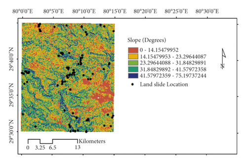
(1) Slope Degree. Slope is one of the important and effective factors on the occurrence of landslides. The reason why the slope variable is important in landslide susceptibility assessment is that it controls surface and subsurface flow and directly affects runoff and infiltration [65]. In the present study, a slope angle map in five classes was prepared from DEM using natural break method of GIS software (Figure 4).

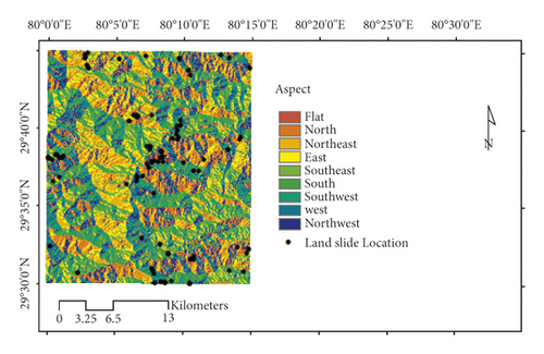
(2) Aspect. The slope aspect is considered as an important parameter in assessing landslide susceptibility [66] as the sun, air/wind and rain/precipitation of the region affect in different directions [67]. On the other hand, aspect indirectly affects the vegetation and soil moisture. In the present study, the slope aspect map is divided into nine classes: flat, north, northeast, east, southeast, south, southwest, west and northwest using DEM (Figure 4).

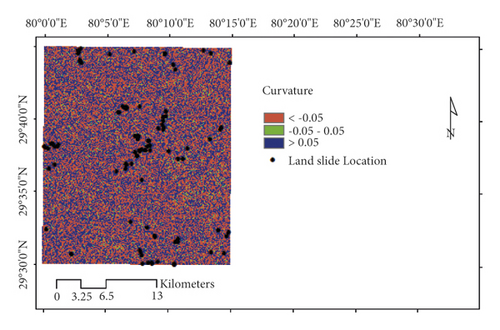
(3) Curvature. Curvature of the slope plays an important role in the surface run off and ground infiltration thus affects the erosion of the surface and ground water condition of the region [66]. Thus, this factor affects the occurrence of landslides. The curvature map of this area was prepared from DEM and classified in the concave, convex and flat surfaces using GIS software (Figure 4).

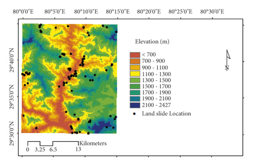
(4) Elevation. Elevation is an important factor in the occurrence of landslides [66]. In general, landslides occur in the hilly areas. At higher elevations generally rains are less but glaciers are prominent. Most of the rains and vegetation is confined at lower and middle elevations in Himalayas. Landslides events depend on the elevation where slopes are moderate to high with heavy rainfall and less vegetation. The study area was divided into nine classes of slopes from DEM using natural break method of Arc GIS (Figure 4).

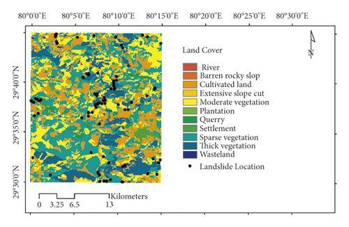
(5) Land Cover. In general, bare lands and unvegetated areas are more prone to landslides than lands with dense vegetation cover and forested areas [68]. In the highly vegetated area roots of plants act as a reinforcement of the ground and prevent erosion. In the dense forest area impact of the rains directly on the ground is very less due to foliage and thus less erosion. Landslides also occur in the cultivated area due to percolation of water during irrigation and also due to erosion of top soil. The land use map of the study area was extracted from the data available from Geological Survey of India report (https://www.gsi.gov.in/webcenter/portal). The land use map of the study area consists of eleven main groups (Figure 4).

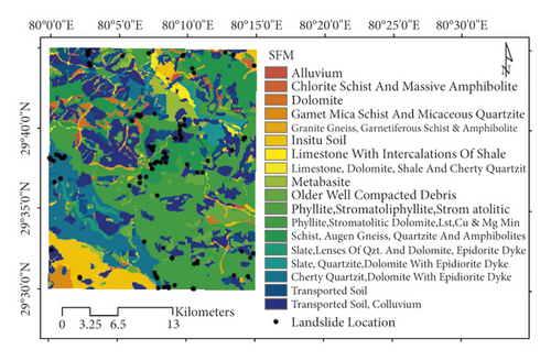
(6) Slope Forming Materials (SFM). The SFM map was extracted from the data available on the Geological Survey of India website (https://www.gsi.gov.in/webcenter/portal). Type of the SFM is very important in the shallow landslide study. Characteristics of the groundmass depend on the SFM; its permeability, porosity and geotechnical properties. Landslides depend on the above characteristics of the material and also on the size and binding/looseness of soil and joints in the rock mass. The SFM map of the present study area was classified into eighteen main groups (Figure 4).

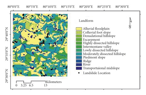
(7) Geomorphology (Landforms). Geomorphology which is a study of landforms is an important factor in the study of landslide susceptibility [18]. Geomorphological features such as mountains, valleys, river terraces, undulating grounds, ridges and escarpments etc., and affects the occurrence of landslides in conjunction with other topographic and geo-environmental factors. The relevant landform factors were extracted from the data available on the Geological Survey of India report (https://www.gsi.gov.in/webcenter/portal) (Figure 4).

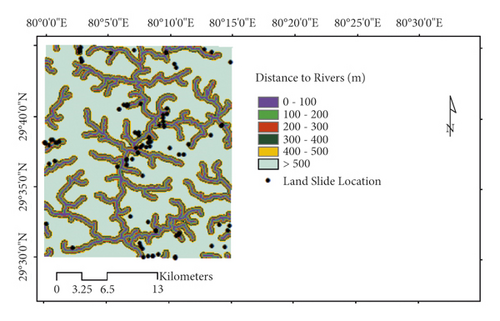
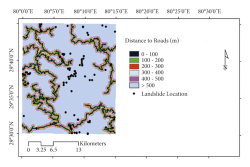
(8) Distance to Rivers and Roads. Distance from roads is one of the anthropogenic factors used in landslide susceptibility assessment. Presence of road network and absence of roads in the area affect landslide occurrences [69]. Roadside excavation and vegetation removal are activities that cause landslides during road construction [43]. Anthropogenic activities such as excavation of roads create instability of slopes near and adjacent to roads up to certain distances depending on the nature of ground mass and geology. Hence, the distance from the road is a very impressive factor in the landslide study [26]. Similarly, distance to rivers also plays an important role in the assessment of landslides for the development of landslide susceptibility maps. The hydrological network regime, soil saturation of water sources, and groundwater recharge, as well as increasing water pressure to empty water pores, lead to landslides in areas adjacent to water sources, rivers and streams [70]. Road distance and river distance buffer maps were prepared for the landslide susceptibility mapping (Figure 4).

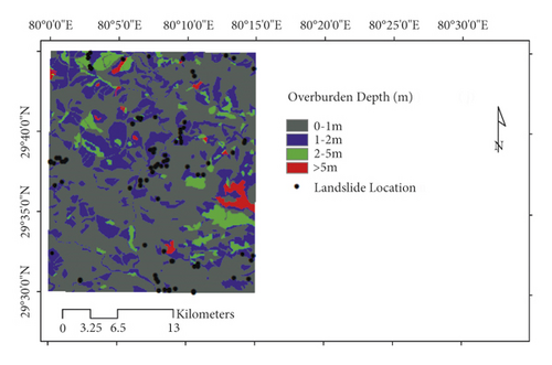
(9) Overburden Depth. Chances of slope failure are more likely in thick overburden areas depending on the characteristics of the overburden material. Major part of the study area is covered thin over burden (1–3 m) with occasional pockets of greater than 5 m. Thus, the possibility of landslides due to failure of overburden material is very less. However, nature and thickness of material affects the infiltration and thus ground water conditions in the area which may affect moisture conditions of the underlying rock mass creating instability and thus landslides. Overburden material map was extracted from the data available on the Geological Survey of India report (https://www.gsi.gov.in/webcenter/portal) (Figure 4).

4. Results and Discussion

4.1. Analysis of WOE and SE Models Results

Table 2 shows the results of landslide susceptibility analysis of landslide affecting factors using the WOE and SE models. The slope analysis results show that the highest number of landslides (60) occurrence are in slope range 41.57°–75.19° in case of both the models. The difference between positive and negative weights (C) in the WOE method and landslide density (P_ij) in the SE method in the moderate to high slope is the highest. As shown by decreasing the degree of weight gradient the presence of landslides decreased. Generally, on the lower slopes of the resistant forces are more than the driving forces and the condition of the landslide occurrence is not favourable.

2. WOE and SE analysis of landslide conditioning factors.

Factors	Class	Class pixels	Landslide pixels	% class pixels	% landslide pixels	WOE			SE
Factors	Class	Class pixels	Landslide pixels	% class pixels	% landslide pixels	W+	W−	C	P_ij	E_j
Slope (^o)	0–14.15	118169	13	15.89	6.31	−0.92	0.11	−1.03	0.06	−0.07
	14.15–23.29	199856	18	26.87	8.74	−1.12	0.22	−1.35	0.05	−0.07
	23.29–31.84	209771	38	28.21	18.45	−0.42	0.13	−0.55	0.10	−0.10
	31.84–41.57	156899	77	21.10	37.38	0.57	−0.23	0.80	0.26	−0.15
	41.57–75.19	59028	60	7.94	29.13	1.30	−0.26	1.56	0.54	−0.15

Aspect	Flat	24	0	0.00	0	0.00	0.00	0.00	0.00	0.00
	North	104954	12	14.11	5.83	−0.88	0.09	−0.98	0.05	−0.07
	Northeast	97075	2	13.05	0.97	−2.60	0.13	−2.73	0.01	−0.02
	East	78103	10	10.50	4.85	−0.77	0.06	−0.83	0.06	−0.07
	Southeast	90944	34	12.23	16.5	0.30	−0.05	0.35	0.17	−0.13
	South	106073	32	14.26	15.53	0.09	−0.01	0.10	0.13	−0.12
	Southwest	95612	44	12.86	21.36	0.51	−0.10	0.61	0.20	−0.14
	West	82462	50	11.09	24.27	0.78	−0.16	0.94	0.27	−0.15
	Northwest	88476	22	11.90	10.68	−0.11	0.01	−0.12	0.11	−0.11

Landforms	Alluvial floodplain	269243	55	36.20	26.70	−0.30	0.14	−0.44	0.05	−0.07
	Colluvial foot slope	19838	17	2.67	8.25	1.13	−0.06	1.19	0.22	−0.14
	Denudational hillslope	12518	10	1.68	4.85	1.06	−0.03	1.09	0.20	−0.14
	Escarpment	5688	1	0.76	0.49	−0.45	0.00	−0.46	0.04	−0.06
	Highly dissected hillslope	48240	23	6.49	11.17	0.54	−0.05	0.59	0.12	−0.11
	Intermontane valley	31136	0	4.19	0.00	0.00	0.04	−0.04	0.00	0.00
	Lowly dissected hillslope	3357	0	0.45	0.00	0.00	0.00	0.00	0.00	0.00
	Moderately dissected hillslope	270620	82	36.39	39.81	0.09	−0.06	0.15	0.08	−0.09
	Piedmont slope	12132	12	1.63	5.83	1.27	−0.04	1.32	0.25	−0.15
	Ridge	47232	5	6.35	2.43	−0.96	0.04	−1.00	0.03	−0.04
	River	119	0	0.02	0.00	0.00	0.00	0.00	0.00	0.00
	Transportational midslope	23600	1	3.17	0.49	−1.88	0.03	−1.91	0.01	−0.02

Curvature	Concave (<−0.05)	358460	128	48.20	62.14	0.25	−0.31	0.57	0.50	−0.15
	Flat (−0.05–0.05)	34132	5	4.59	2.43	−0.64	0.02	−0.66	0.21	−0.14
	Convex (>0.05)	351131	73	47.21	35.44	−0.29	0.20	−0.49	0.29	−0.16

SFM	Alluvium	6244	0	0.84	0	0.00	0.01	−0.01	0.00	0.00
	Chlorite schist and massive amphibolite	2707	0	0.36	0	0.00	0.00	0.00	0.00	0.00
	Dolomite	11602	1	1.56	0.49	0.00	0.02	−0.02	0.03	−0.05
	Garnet mica schist and micaceous quartzite	5469	0	0.74	0	0.00	0.01	−0.01	0.00	0.00
	Granite Gneiss, Garnetiferous schist and amphibolite	18402	3	2.47	1.46	−0.53	0.01	−0.54	0.06	−0.08
	Insitu soil	45822	3	6.16	1.46	−1.44	0.05	−1.49	0.03	−0.04
	Limestone with intercalations of shale	5052	0	0.68	0	0.00	0.01	−0.01	0.00	0.00
	Limestone, dolomite, shale and cherty quartzit	4327	0	0.58	0	0.00	0.01	−0.01	0.00	0.00
	Metabasite	18692	1	2.51	0.49	−1.64	0.02	−1.67	0.02	−0.04
	Older well compacted debris	46657	1	6.27	0.49	−2.56	0.06	−2.62	0.01	−0.02
	Phyllite, Stromatoliphyllite,Stromatolitic	391	0	0.05	0	0.00	0.00	0.00	0.00	0.00
	Phyllite, Stromatolitic Dolomite,Lst, Cu and Mg min.	209799	50	28.21	24.27	−0.15	0.05	−0.20	0.09	−0.10
	Schist, augen gneiss, quartzite and amphibolites	83168	43	11.18	20.87	0.62	−0.12	0.74	0.20	−0.14
	Slate, Lenses of qzt. And dolomite, epidorite dyke	6583	0	0.89	0	0.00	0.01	−0.01	0.00	0.00
	Slate, Quartzite, Dolomite with epidiorite dyke	16086	0	2.16	0	0.00	0.02	−0.02	0.00	0.00
	Cherty Quartzit, Dolomite with epidiorite dykes	75424	67	10.14	32.52	1.17	−0.29	1.45	0.35	−0.16
	Transported soil	52795	21	7.10	10.19	0.36	−0.03	0.40	0.16	−0.13
	Transported soil, colluvium	134503	16	18.09	7.77	−0.85	0.12	−0.96	0.05	−0.06

Land cover	River	96	0	0.01	0	0.00	0.00	0.00	0.00	0.00
	Barren rocky slop	269	0	0.04	0	0.00	0.00	0.00	0.00	0.00
	Cultivated land	164224	35	22.08	16.99	−0.26	0.06	−0.33	0.08	−0.08
	Extensive slope cut	11006	3	1.48	1.46	−0.02	0.00	−0.02	0.10	−0.10
	Moderate vegetation	162678	45	21.87	21.84	0.00	0.00	0.00	0.10	−0.10
	Plantation	2865	1	0.39	0.49	0.23	0.00	0.23	0.12	−0.11
	Settlement	14667	0	1.97	0	0.00	0.02	−0.02	0.00	0.00
	Querry	15136	19	2.04	9.22	1.51	−0.08	1.59	0.44	−0.16
	Sparse vegetation	266609	89	35.85	43.2	0.19	−0.12	0.31	0.12	−0.11
	Thick vegetation	104103	14	14.00	6.8	−0.72	0.08	−0.80	0.05	−0.06
	Wasteland	2053	0	0.28	0	0.00	0.00	0.00	0.00	0.00

Distance to roads (m)	0–100	67380	34	9.06	16.50	0.18	−0.46	0.63	0.49	−0.15
	100–200	57028	11	7.67	5.34	0.60	−0.09	0.69	0.19	−0.14
	200–300	49354	0	6.64	0.00	−0.36	0.02	−0.39	0.00	0.00
	300–400	43581	0	5.86	0.00	0.00	0.07	−0.07	0.00	0.00
	400–500	39241	0	5.28	0.00	0.00	0.06	−0.06	0.00	0.00
	>500	487139	161	65.50	78.16	0.00	0.05	−0.05	0.32	−0.16

Overburden depth (m)	0–1	480051	163	64.55	79.13	0.00	0.02	−0.02	0.43	−0.16
	1–2	203003	28	27.30	13.59	0.20	−0.53	0.73	0.18	−0.13
	2–5	48078	15	6.46	7.28	−0.70	0.17	−0.87	0.40	−0.16
	>5	12591	0	1.69	0	0.12	−0.01	0.13	0.00	0.00

Distance to rivers (m)	0–100	68250	7	9.18	3.4	0.09	−0.13	0.22	0.07	−0.08
	100–200	65780	19	8.84	9.22	−0.99	0.06	−1.06	0.19	−0.14
	200–300	63677	12	8.56	5.83	0.04	0.00	0.05	0.12	−0.11
	300–400	61359	18	8.25	8.74	−0.39	0.03	−0.41	0.19	−0.14
	400–500	58804	21	7.91	10.19	0.00	−0.01	0.01	0.23	−0.15
	>500	425853	129	57.26	62.62	0.00	−0.03	0.03	0.20	−0.14

Elevation (m)	<700	41938	5	5.64	2.43	−0.84	0.03	−0.88	0.05	−0.06
	700–900	69721	51	9.37	24.76	0.97	−0.19	1.16	0.30	−0.16
	900–1100	103488	83	13.91	40.29	1.06	−0.37	1.43	0.33	−0.16
	1100–1300	128838	36	17.32	17.48	0.01	0.00	0.01	0.12	−0.11
	1300–1500	145497	16	19.56	7.77	−0.92	0.14	−1.06	0.05	−0.06
	1500–1700	127267	2	17.11	0.97	−2.87	0.18	−3.05	0.01	−0.01
	1700–1900	79239	0	10.65	0	0.00	0.11	−0.11	0.00	0.00
	1900–2100	35169	13	4.73	6.31	0.29	−0.02	0.31	0.15	−0.12
	2100–2427	12566	0	1.69	0.00	0.00	0.02	−0.02	0.00	0.00

The maximum number of landslides is in the direction of the west aspect with 50 and the highest numerical value of C = 0.94 and P_ij = 0.27 based on the WOE and SE ways is related to the west aspect, respectively. After that, in the southwest, southeast, and south directions of the study area, the highest number of landslides (44, 34, and 32) has been seen, which can be attributed to climatic conditions such as high humidity, which is consistent with the results of other research [27].

The effect of landforms variable on landslide susceptibility in the case area shows that the highest number of landslides on the moderately dissected hills slope formation occurred due to large area, but according to the WOE and SE methods, the highest weight was related to “Piedmont slope” formation with C = 1.32 and the density (P_ij) is 0.25. Also, in the Colluvial foot slope and “Denudational hillslope” formations, there was the highest landslide weight C and density (P_ij), and conversely, there was no landslide susceptibility on the “River” class. In general, it can be stated that rock areas are more resistant to weathering and dispersal so landslides are less likely to occur [71]. But, the geological formations of each region are unique, so the results of the relationship between landslides occur and in different geological formations are various and specific to each region.

The results of curvature (topographic morphology) show that the highest landslide susceptibility is related to concave slopes and convex slopes has less susceptibility and finally flat slopes have the lowest susceptibility. Typically, the positive curvature of a convex topography is upward and the negative curvature of a concave topography is upward. That is, according to the WOE and SE methods, the maximum values of (C = 0.57, −0.49 and −0.66) and (P_ij = 0.50, 0.29 and 0.21) are related to “Concave,” “Convex,” and “Flat” classes, respectively. Negative topographies hold more water and retain water due to rainfall for longsome cycle of time during rainfall than with positively curved slopes, resulting in increased soil wet [72].

The SFM is the most sensitive component of the slope relative to the landslide in the area studied by “Cherty Quartzit, Dolomite with Epidiorite Dykes”, this type of material contributing to the highest number of landslide (67) and also the highest weight landslide (C = 1.45) and density landslide (P_ij = 0.35) in accordance with the WOE and SE methods, respectively. The SFM is an another unique feature of each region and offers different results in different regions.

Most of the study area belongs to “Sparse vegetation”, so it seems quite logical that there are 89 landslides in this land cover. On the other hand, the highest weight (C = 1.59) and density of landslides (P_ij = 0.44) based on two algorithms (WOE and SE) is related to “Querry” land cover. The number and weight of landslides in areas covered with vegetation is higher, which is consistent with previous research [73]. Conversely, in the study area on landscaping where there is stagnant water, hard and rocky areas and habitats such as “River,” “Barren rocky slope,” “Wasteland,” and “Settlement” classes, the number of landslides is zero.

Roads have a great impact on landslides [55]. In the present area, with a distance from the roads, the distance of more than 500 meters, the number of landslides has increased a lot, which is due to the expansion of the area, and on the other hand, at distances of 100–200 meters from the road, the amount of landslide weight (C = 0.69) is more and at distances less than 100 meters, the landslide density (P_ij = 0.49) is the highest according to the WOE and SE algorithms, respectively. In general, man-made and road construction manipulations increase the occurrence of landslides, which our results have similar results with other investigations [27, 74].

The highest number of landslides occurred in the first floor (0–1 m) of the “Overburden depth” variable with a value of 163 and then in the 1–2 m, 2–5 m and >5 m depths the highest number of landslides was observed. Also, the highest weight (C = 0.73) and density of landslides (P_ij = 0.40) with the WOE and SE methods are related to depths of 1–2 and 2–5 meters, respectively.

From the effect of the distance to rivers landslide information layer, it can be seen that the highest number of landslides occurred at a distance of more than 500 meters due to the area, while the maximum weight (C = 0.22) and density (P_ij = 0.23) according to the WOE and SE methods, the distance between 0–100 meters and 400–500 meters from the rivers has been seen on the floor, respectively. Increasing humidity through distance from the river can affect the occurrence of landslides and create a high correlation with the presence of landslides. The results of this variable based on the WOE and its correlation with landslide occurrence are consistent with Pourghasemi, Pradhan, Gokceoglu, Mohammadi, and Moradi [27] study.

The results of the relationship between different classes of elevation and the occurrence of landslides indicate that in the third classes (900–1100 meters) has the highest number (83), weight (C = 1.43) and density (P_ij = 0.33) of landslides according to both algorithms (WOE and SE). Since in the present study the highest incidence of landslides compared to altitude classes landslide occurrence in the third floor out of 9 floors shows that in the lower floor was the most sensitive to landslides and it can be seen that this factor has little effect on landslides susceptibility and other factors play a greater role in landslides and since the landslide occurs at high altitudes, the different result may be that in the high altitudes of the area the study is due to the rocky nature of the region, which has not occurred on the last floor, the highest elevation of the landslide [39]. Some researchers used altitude as a controlling factor in the occurrence of landslides [75].

In general, the causes of landslides are many, complex and sometimes unknown. Although the underlying factors influencing landslide occurrence can be observed during field visits, aerial photo interpretation, and satellite imagery. Several geomorphometric factors are involved in the analysis to investigate the effective factors in landslide occurrence [76]. Quantitative measurement of many geomorphometric factors by field visits is difficult and therefore it is difficult to know their relationship to the occurrence of landslide mechanism. Because landslides are among the most devastating natural disasters, many researchers around the world have attempted to assess landslide hazards, identify hazardous areas, and display their spatial distribution by indirect methods [20]. In this study, Google Earth images, DEM data and Geological Survey of India maps have been used for the development of landslide susceptibility maps using the WOE and SE, which is an effective approach for landslide study in regional scale.

4.2. Development of Landslide Susceptibility Maps

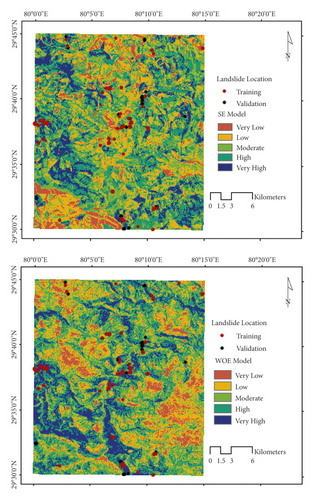
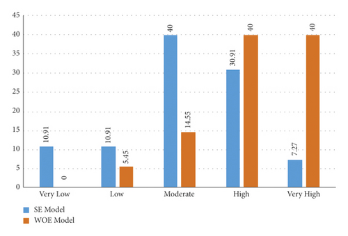
Weights of each classes of the factors generated from the WOE and SE methods (Table 2) were used to generate landslide susceptibility maps of the study area using GIS application (Figure 5). Natural break classification method was used to classify the landslide susceptibility indices into five classes. Figure 6 shows the percentage distribution of landslide pixels in five landslide susceptibility classes “very low, low, moderate, high and very high” based on both SE and WOE algorithms. In the very low susceptibility class, 10.91% of the study area is affected by landslide susceptibility according to the SE and almost negligible according to the WOE model. In the low susceptibility class, 10.91% and 5.45% of the area affected by landslides according to the SE and WOE methods, respectively. On the other hand, in the moderate susceptibility class, 40% and 14.55% of the study area is affected according to the SE and WOE methods, respectively. Also, in the high susceptibility class, 30.91% area and 40% area is affected according to the SE and WOE methods, respectively. Whereas, in the high susceptibility class, 7.27% and 40% area is affected according to the SE and WOE methods, respectively. The analysis indicated the WOE method gave high distribution (40%) of landslides in both high and vey high susceptibility class compared with those of the SE method.

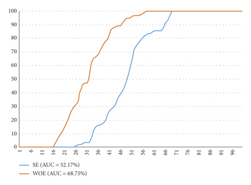
In this study, the ROC curve was used to evaluate the bivariate statistical models: SE and WOE (Figure 7). Area under this curve of the SE model is 52.17 (AUC_SE) and of the WOE model is 68.75 (AUC_WOE) which means weak accuracy of prediction of the SE model and moderate of the WOE model in the development of landslide susceptibility zone maps (Figure 7). The results of the accuracy of the method WOE compared to another method are consistent with other researchers [40, 55, 71]; however, their performance is lower than other ML models using the same dataset such as Naïve Bayes (AUC = 0.873), Multilayer Perceptron neural network classifier (AUC = 0.864), and Alternating Decision Tree (AUC = 0.840). One of the advantages of these two-variable statistical methods is that in these models, data collection and analysis is relatively easy and requires little time to do it.

4.3. Validation of Landslide Susceptibility Models

In this study, the ROC curve was used to evaluate the bivariate statistical models: SE and WOE (Figure 7). Area under this curve of the SE model is 52.17 (AUC_SE) and of the WOE model is 68.75 (AUC_WOE) which means weak accuracy of prediction of the SE model and moderate of the WOE model in the development of landslide susceptibility zone maps (Figure 7). The results of the accuracy of the method WOE compared to another method are consistent with other researchers [40, 55, 71]. One of the advantages of these two-variable statistical methods is that in these models, data collection and analysis is relatively easy and requires little time to do it.

5. Conclusion

In the present study, performances of the two simple popular bivariate statistical models (SE and WOE) have been evaluated for developing landslide susceptibility maps of Pithoragadh district, Uttarakhand state, India. The AUC ROC results indicated that WOE model (AUC_WOE = 68.75) is better than the SE model (AUC_SE = 52.17). Even though the AUC values of the models are not high, they are acceptable for landslide susceptibility mapping, as the landslide classes boundaries are not regular in Himalayan region and depends on heterogeneous topographical and geological features. Thus, WOE model having better performance can be used for the identification of landslide susceptible zones which can be used for the land use planning and prevention of landslides in hilly and mountainous areas not only Himalayas but other parts of the world also. Nowadays, ML methods are being applied for model studies in landslide susceptibility mapping. It is proposed to carryout Machine Learning model studies in this area and compare the results with bivariate statistical models for further improvement of performance considering more input parameters.

Conflicts of Interest

The authors declare that they have no conflicts of interest.

Acknowledgments

The authors thank the University of Transport Technology, Hanoi, Vietnam, for supporting this research.

Open Research

Data Availability

The data used to support the findings of this study are available from the corresponding author upon request.

References

1 Lazzari M., Gioia D., and Anzidei B., Landslide inventory of the Basilicata region (southern Italy), Journal of Maps. (2018) 14, no. 2, 348–356, https://doi.org/10.1080/17445647.2018.1475309, 2-s2.0-85054678065.
10.1080/17445647.2018.1475309
Web of Science® Google Scholar
2 Keesstra S. D., Bouma J., Wallinga J., Tittonell P., Smith P., Cerdà A., Montanarella L., Quinton J. N., Pachepsky Y., and van der Putten W. H., The significance of soils and soil science towards realization of the United Nations Sustainable Development Goals, Soils. (2016) 2, no. 2, 111–128, https://doi.org/10.5194/soil-2-111-2016, 2-s2.0-85034611088.
10.5194/soil-2-111-2016
Web of Science® Google Scholar
3 Keesstra S., Mol G., De Leeuw J., Okx J., De Cleen M., and Visser S., Soil-related sustainable development goals: four concepts to make land degradation neutrality and restoration work, Land. (2018) 7, no. 4, https://doi.org/10.3390/land7040133, 2-s2.0-85058126581.
10.3390/land7040133
Web of Science® Google Scholar
4 Visser S., Keesstra S., Maas G., and De Cleen M., Soil as a basis to create enabling conditions for transitions towards sustainable land management as a key to achieve the SDGs by 2030, Sustainability. (2019) 11, no. 23, https://doi.org/10.3390/su11236792.
10.3390/su11236792
Web of Science® Google Scholar
5 Crozier M. J., E. Geology, Landslides, 1999, Springer Netherlands, Dordrecht, 371–375.
Google Scholar
6 Corominas J. and Moya J., A review of assessing landslide frequency for hazard zoning purposes, Engineering Geology. (2008) 102, no. 3, 193–213, https://doi.org/10.1016/j.enggeo.2008.03.018, 2-s2.0-56249098302.
10.1016/j.enggeo.2008.03.018
Web of Science® Google Scholar
7 Gariano S. L. and Guzzetti F., Landslides in a changing climate, Earth-Science Reviews. (2016) 162, 227–252, https://doi.org/10.1016/j.earscirev.2016.08.011, 2-s2.0-84989935664.
10.1016/j.earscirev.2016.08.011
Web of Science® Google Scholar
8 Chen W., Shirzadi A., Shahabi H., Ahmad B. B., Zhang S., Hong H., and Zhang N., A novel hybrid artificial intelligence approach based on the rotation forest ensemble and naïve Bayes tree classifiers for a landslide susceptibility assessment in Langao County, China, Geomatics, Natural Hazards and Risk. (2017) 8, no. 2, 1955–1977, https://doi.org/10.1080/19475705.2017.1401560, 2-s2.0-85034255369.
10.1080/19475705.2017.1401560
Web of Science® Google Scholar
9 Nsengiyumva J. B., Luo G., Amanambu A. C., Mind’je R., Habiyaremye G., Karamage F., Ochege F. U., and Mupenzi C., Comparing probabilistic and statistical methods in landslide susceptibility modeling in Rwanda/Centre-Eastern Africa, The Science of the Total Environment. (2018) 659, 1457–1472, https://doi.org/10.1016/j.scitotenv.2018.12.248, 2-s2.0-85059577517.
10.1016/j.scitotenv.2018.12.248
PubMed Web of Science® Google Scholar
10 Ozer B. C., Mutlu B., Nefeslioglu H. A., Sezer E. A., Rouai M., Dekayir A., and Gokceoglu C., On the use of hierarchical fuzzy inference systems (HFIS) in expert-based landslide susceptibility mapping: the central part of the Rif Mountains (Morocco), Bulletin of Engineering Geology and the Environment. (2020) 79, no. 1, 551–568, https://doi.org/10.1007/s10064-019-01548-5, 2-s2.0-85067284800.
10.1007/s10064-019-01548-5
Web of Science® Google Scholar
11 Corominas J., Copons R., Vilaplana J. M., Altimir J., and Amigó J., Integrated landslide susceptibility analysis and hazard assessment in the principality of Andorra, Natural Hazards. (2003) 30, no. 3, 421–435, https://doi.org/10.1023/b:nhaz.0000007094.74878.d3, 2-s2.0-0742305101.
10.1023/B:NHAZ.0000007094.74878.d3
Web of Science® Google Scholar
12 De Sy V., Schoorl J., Keesstra S., Jones K., and Claessens L., Landslide model performance in a high resolution small-scale landscape, Geomorphology. (2013) 190, 73–81, https://doi.org/10.1016/j.geomorph.2013.02.012, 2-s2.0-84876099147.
10.1016/j.geomorph.2013.02.012
Web of Science® Google Scholar
13 Shirzadi A., Solaimani K., Roshan M. H., Kavian A., Chapi K., Shahabi H., Keesstra S., Ahmad B. B., and Bui D. T., Uncertainties of prediction accuracy in shallow landslide modeling: sample size and raster resolution, Catena. (2019) 178, 172–188, https://doi.org/10.1016/j.catena.2019.03.017, 2-s2.0-85062906050.
10.1016/j.catena.2019.03.017
Web of Science® Google Scholar
14 Achour Y., Boumezbeur A., Hadji R., Chouabbi A., Cavaleiro V., and Bendaoud E. A., Landslide susceptibility mapping using analytic hierarchy process and information value methods along a highway road section in Constantine, Algeria, Arabian Journal of Geosciences. (2017) 10, no. 8, https://doi.org/10.1007/s12517-017-2980-6, 2-s2.0-85018475644.
10.1007/s12517-017-2980-6
Web of Science® Google Scholar
15 Pham Q. B., Achour Y., Ali S. A., Parvin F., Vojtek M., Vojteková J., Al-Ansari N., Achu A., Costache R., and Khedher K. M., A comparison among fuzzy multi-criteria decision making, bivariate, multivariate and machine learning models in landslide susceptibility mapping, Geomatics, Natural Hazards and Risk. (2021) 12, no. 1, 1741–1777, https://doi.org/10.1080/19475705.2021.1944330.
10.1080/19475705.2021.1944330
Web of Science® Google Scholar
16 Achour Y., Saidani Z., Touati R., Pham Q. B., Pal S. C., Mustafa F., and Balik Sanli F., Assessing landslide susceptibility using a machine learning-based approach to achieving land degradation neutrality, Environmental Earth Sciences. (2021) 80, no. 17, 1–20, https://doi.org/10.1007/s12665-021-09889-9.
10.1007/s12665-021-09889-9
Web of Science® Google Scholar
17 Liu J. and Duan Z., Quantitative assessment of landslide susceptibility comparing statistical index, index of entropy, and weights of evidence in the shangnan area, China, Entropy. (2018) 20, no. 11, https://doi.org/10.3390/e20110868, 2-s2.0-85057006672.
10.3390/e20110868
Web of Science® Google Scholar
18 Shirani K., Pasandi M., and Arabameri A., Landslide susceptibility assessment by dempster–shafer and index of entropy models, sarkhoun basin, southwestern Iran, Natural Hazards. (2018) 93, no. 3, 1379–1418, https://doi.org/10.1007/s11069-018-3356-2, 2-s2.0-85047180518.
10.1007/s11069-018-3356-2
Web of Science® Google Scholar
19 Sun X., Chen J., Bao Y., Han X., Zhan J., and Peng W., Landslide susceptibility mapping using logistic regression analysis along the jinsha river and its tributaries close to derong and deqin county, southwestern China, ISPRS International Journal of Geo-Information. (2018) 7, no. 11, https://doi.org/10.3390/ijgi7110438, 2-s2.0-85058009644.
10.3390/ijgi7110438
PubMed Web of Science® Google Scholar
20 Chen W., Zhang S., Li R., and Shahabi H., Performance evaluation of the GIS-based data mining techniques of best-first decision tree, random forest, and naïve Bayes tree for landslide susceptibility modeling, The Science of the Total Environment. (2018) 644, 1006–1018, https://doi.org/10.1016/j.scitotenv.2018.06.389, 2-s2.0-85049596640.
10.1016/j.scitotenv.2018.06.389
CAS PubMed Web of Science® Google Scholar
21 Reichenbach P., Busca C., Mondini A. C., and Rossi M., The influence of land use change on landslide susceptibility zonation: the Briga catchment test site (Messina, Italy), Environmental Management. (2014) 54, no. 6, 1372–1384, https://doi.org/10.1007/s00267-014-0357-0, 2-s2.0-84911439849.
10.1007/s00267-014-0357-0
CAS PubMed Web of Science® Google Scholar
22 Felicísimo Á. M., Cuartero A., Remondo J., and Quirós E., Mapping landslide susceptibility with logistic regression, multiple adaptive regression splines, classification and regression trees, and maximum entropy methods: a comparative study, Landslides. (2013) 10, no. 2, 175–189, https://doi.org/10.1007/s10346-012-0320-1, 2-s2.0-84875731577.
10.1007/s10346-012-0320-1
Web of Science® Google Scholar
23 Shahabi H. and Hashim M., Landslide susceptibility mapping using GIS-based statistical models and Remote sensing data in tropical environment, Scientific Reports. (2015) 5, no. 1, 9899, https://doi.org/10.1038/srep09899, 2-s2.0-84928712005.
10.1038/srep09899
CAS PubMed Web of Science® Google Scholar
24 Raman R. and Punia M., The application of GIS-based bivariate statistical methods for landslide hazards assessment in the upper Tons river valley, Western Himalaya, India, Georisk: Assessment and Management of Risk for Engineered Systems and Geohazards. (2012) 6, no. 3, 145–161, https://doi.org/10.1080/17499518.2011.637504, 2-s2.0-84864650673.
10.1080/17499518.2011.637504
Google Scholar
25 Aghdam I. N., Varzandeh M. H. M., and Pradhan B., Landslide susceptibility mapping using an ensemble statistical index (Wi) and adaptive neuro-fuzzy inference system (ANFIS) model at Alborz Mountains (Iran), Environmental Earth Sciences. (2016) 75, no. 7, https://doi.org/10.1007/s12665-015-5233-6, 2-s2.0-84961683938.
10.1007/s12665-015-5233-6
Web of Science® Google Scholar
26 Devkota K. C., Regmi A. D., Pourghasemi H. R., Yoshida K., Pradhan B., Ryu I. C., Dhital M. R., and Althuwaynee O. F., Landslide susceptibility mapping using certainty factor, index of entropy and logistic regression models in GIS and their comparison at Mugling–Narayanghat road section in Nepal Himalaya, Natural Hazards. (2013) 65, no. 1, 135–165, https://doi.org/10.1007/s11069-012-0347-6, 2-s2.0-84870822749.
10.1007/s11069-012-0347-6
Web of Science® Google Scholar
27 Pourghasemi H. R., Pradhan B., Gokceoglu C., Mohammadi M., and Moradi H. R., Application of weights-of-evidence and certainty factor models and their comparison in landslide susceptibility mapping at Haraz watershed, Iran, Arabian Journal of Geosciences. (2013) 6, no. 7, 2351–2365, https://doi.org/10.1007/s12517-012-0532-7, 2-s2.0-84879580121.
10.1007/s12517-012-0532-7
Web of Science® Google Scholar
28 Chung C.-J. F., Fabbri A. G., Jang D.-H., and Scholten H. J., P. van Oosterom, S. Zlatanova, and E. M. Fendel, Risk assessment using spatial prediction model for natural disaster preparedness Geo-information for Disaster Management, 2005, Springer, Berlin, Heidelberg, 619–640, https://doi.org/10.1007/3-540-27468-5_45, 2-s2.0-85072045369.
10.1007/3-540-27468-5_45
Google Scholar
29 Carranza E. J. M. and Hale M., Geologically constrained probabilistic mapping of gold potential, baguio district, Philippines, Natural Resources Research. (2000) 9, no. 3, 237–253, https://doi.org/10.1023/a:1010147818806, 2-s2.0-52649157492.
10.1023/A:1010147818806
Google Scholar
30 Guzzetti F., Reichenbach P., Ardizzone F., Cardinali M., and Galli M., Estimating the quality of landslide susceptibility models, Geomorphology. (2006) 81, no. 1, 166–184, https://doi.org/10.1016/j.geomorph.2006.04.007, 2-s2.0-33749586744.
10.1016/j.geomorph.2006.04.007
Web of Science® Google Scholar
31 Pradhan B., Chaudhari A., Adinarayana J., and Buchroithner M. F., Soil erosion assessment and its correlation with landslide events using remote sensing data and GIS: a case study at Penang Island, Malaysia, Environmental Monitoring and Assessment. (2012) 184, no. 2, 715–727, https://doi.org/10.1007/s10661-011-1996-8, 2-s2.0-85027941774.
10.1007/s10661-011-1996-8
PubMed Web of Science® Google Scholar
32 Wan S., Lei T. C., and Chou T. Y., Optimized object-based image classification: development of landslide knowledge decision support system, Arabian Journal of Geosciences. (2014) 7, no. 5, 2059–2070, https://doi.org/10.1007/s12517-013-0952-z, 2-s2.0-84899529110.
10.1007/s12517-013-0952-z
Web of Science® Google Scholar
33 Tangestani M. H., A comparative study of Dempster–Shafer and fuzzy models for landslide susceptibility mapping using a GIS: an experience from Zagros Mountains, SW Iran, Journal of Asian Earth Sciences. (2009) 35, no. 1, 66–73, https://doi.org/10.1016/j.jseaes.2009.01.002, 2-s2.0-61449099321.
10.1016/j.jseaes.2009.01.002
Web of Science® Google Scholar
34 Oh H.-J. and Lee S., Cross-application used to validate landslide susceptibility maps using a probabilistic model from Korea, Environmental Earth Sciences. (2011) 64, no. 2, 395–409, https://doi.org/10.1007/s12665-010-0864-0, 2-s2.0-80052070589.
10.1007/s12665-010-0864-0
Web of Science® Google Scholar
35 Neuhäuser B. and Terhorst B., Landslide susceptibility assessment using “weights-of-evidence” applied to a study area at the Jurassic escarpment (SW-Germany), Geomorphology. (2007) 86, no. 1, 12–24, https://doi.org/10.1016/j.geomorph.2006.08.002, 2-s2.0-33947723369.
10.1016/j.geomorph.2006.08.002
Web of Science® Google Scholar
36 Park N.-W., Application of Dempster-Shafer theory of evidence to GIS-based landslide susceptibility analysis, Environmental Earth Sciences. (2011) 62, no. 2, 367–376, https://doi.org/10.1007/s12665-010-0531-5, 2-s2.0-78650997072.
10.1007/s12665-010-0531-5
PubMed Web of Science® Google Scholar
37 Ali S. A., Parvin F., Vojteková J., Costache R., Linh N. T. T., Pham Q. B., Vojtek M., Gigović L., Ahmad A., and Ghorbani M. A., GIS-based landslide susceptibility modeling: a comparison between fuzzy multi-criteria and machine learning algorithms, Geoscience Frontiers. (2020) 12, 857–876, https://doi.org/10.1016/j.gsf.2020.09.004.
10.1016/j.gsf.2020.09.004
Web of Science® Google Scholar
38 Arca D., Kutoğlu H., and Becek K., Landslide susceptibility mapping in an area of underground mining using the multicriteria decision analysis method, Environmental Monitoring and Assessment. (2018) 190, no. 12, https://doi.org/10.1007/s10661-018-7085-5, 2-s2.0-85056594558.
10.1007/s10661-018-7085-5
PubMed Web of Science® Google Scholar
39 Chen W., Fan L., Li C., and Pham B. T., Spatial prediction of landslides using hybrid integration of artificial intelligence algorithms with frequency ratio and index of entropy in nanzheng county, China, Applied Sciences. (2020) 10, no. 1, https://doi.org/10.3390/app10010029.
10.3390/app10010029
Google Scholar
40 Sifa S. F., Mahmud T., Tarin M. A., and Haque D. M. E., Event-based landslide susceptibility mapping using weights of evidence (WoE) and modified frequency ratio (MFR) model: a case study of Rangamati district in Bangladesh, Geology, Ecology, and Landscapes. (2020) 4, no. 3, 222–235, https://doi.org/10.1080/24749508.2019.1619222.
10.1080/24749508.2019.1619222
Google Scholar
41 Tien Bui D., Pradhan B., Lofman O., Revhaug I., and Dick O. B., Landslide susceptibility mapping at Hoa Binh province (Vietnam) using an adaptive neuro-fuzzy inference system and GIS, Computers & Geosciences. (2012) 45, 199–211, https://doi.org/10.1016/j.cageo.2011.10.031, 2-s2.0-84863487918.
10.1016/j.cageo.2011.10.031
Web of Science® Google Scholar
42 Pham B. T., Pradhan B., Tien Bui D., Prakash I., and Dholakia M. B., A comparative study of different machine learning methods for landslide susceptibility assessment: a case study of Uttarakhand area (India), Environmental Modelling & Software. (2016) 84, 240–250, https://doi.org/10.1016/j.envsoft.2016.07.005, 2-s2.0-84989813944.
10.1016/j.envsoft.2016.07.005
Web of Science® Google Scholar
43 Sameen M. I., Sarkar R., Pradhan B., Drukpa D., Alamri A. M., and Park H.-J., Landslide spatial modelling using unsupervised factor optimisation and regularised greedy forests, Computers & Geosciences. (2020) 134, 104336, https://doi.org/10.1016/j.cageo.2019.104336.
10.1016/j.cageo.2019.104336
Web of Science® Google Scholar
44 Kavzoglu T., Kutlug Sahin E., and Colkesen I., Selecting optimal conditioning factors in shallow translational landslide susceptibility mapping using genetic algorithm, Engineering Geology. (2015) 192, 101–112, https://doi.org/10.1016/j.enggeo.2015.04.004, 2-s2.0-84928157611.
10.1016/j.enggeo.2015.04.004
Web of Science® Google Scholar
45 Paul S., Bartarya S., Rautela P., and Mahajan A., Catastrophic mass movement of 1998 monsoons at Malpa in kali valley, kumaun himalaya (India), Geomorphology. (2000) 35, no. 3-4, 169–180, https://doi.org/10.1016/s0169-555x(00)00032-5, 2-s2.0-0033744665.
10.1016/S0169-555X(00)00032-5
Web of Science® Google Scholar
46 Shannon C. E., A mathematical theory of communication, The Bell System Technical Journal. (1948) 27, no. 3, 379–423, https://doi.org/10.1002/j.1538-7305.1948.tb01338.x, 2-s2.0-84940644968.
10.1002/j.1538-7305.1948.tb01338.x
Web of Science® Google Scholar
47 Constantin M., Bednarik M., Jurchescu M. C., and Vlaicu M., Landslide susceptibility assessment using the bivariate statistical analysis and the index of entropy in the Sibiciu Basin (Romania), Environmental Earth Sciences. (2011) 63, no. 2, 397–406, https://doi.org/10.1007/s12665-010-0724-y, 2-s2.0-79955062758.
10.1007/s12665-010-0724-y
Web of Science® Google Scholar
48 Mahmoud S. H. and Alazba A. A., Integrated remote sensing and GIS-based approach for deciphering groundwater potential zones in the central region of Saudi Arabia, Environmental Earth Sciences. (2016) 75, no. 4, https://doi.org/10.1007/s12665-015-5156-2, 2-s2.0-84958036264.
10.1007/s12665-015-5156-2
Web of Science® Google Scholar
49 Bednarik M., Magulová B., Matys M., and Marschalko M., Landslide susceptibility assessment of the Kraľovany–Liptovský Mikuláš railway case study, Physics and Chemistry of the Earth, Parts A/B/C. (2010) 35, no. 3, 162–171, https://doi.org/10.1016/j.pce.2009.12.002, 2-s2.0-77953026730.
10.1016/j.pce.2009.12.002
Web of Science® Google Scholar
50 Hong H., Ilia I., Tsangaratos P., Chen W., and Xu C., A hybrid fuzzy weight of evidence method in landslide susceptibility analysis on the Wuyuan area, China, Geomorphology. (2017) 290, 1–16, https://doi.org/10.1016/j.geomorph.2017.04.002, 2-s2.0-85017564282.
10.1016/j.geomorph.2017.04.002
Web of Science® Google Scholar
51 Goodman J. E., Zu K., Loftus C. T., Lynch H. N., Prueitt R. L., Mohar I., Shubin S. P., and Sax S. N., Short-term ozone exposure and asthma severity: weight-of-evidence analysis, Environmental Research. (2018) 160, 391–397, https://doi.org/10.1016/j.envres.2017.10.018, 2-s2.0-85032864671.
10.1016/j.envres.2017.10.018
CAS PubMed Web of Science® Google Scholar
52 García-Pérez C., Prieto-Alaiz M., and Simón H., Multidimensional measurement of precarious employment using hedonic weights: evidence from Spain, Journal of Business Research. (2020) 113, 348–359.
10.1016/j.jbusres.2019.09.036
Web of Science® Google Scholar
53 Rosenblatt E., E. Rosenblatt, Chapter Twelve - calculating weight of evidence and information value Credit Data and Scoring, 2020, Academic Press, Cambridge, MA, USA, 99–104, https://doi.org/10.1016/b978-0-12-818815-6.00012-1.
10.1016/B978-0-12-818815-6.00012-1
Google Scholar
54 Shirzadi A., Soliamani K., Habibnejhad M., Kavian A., Chapi K., Shahabi H., Chen W., Khosravi K., Thai Pham B., Pradhan B., Ahmad A., Bin Ahmad B., and Tien Bui D., Novel GIS based machine learning algorithms for shallow landslide susceptibility mapping, Sensors. (2018) 18, no. 11, https://doi.org/10.3390/s18113777, 2-s2.0-85056263734.
10.3390/s18113777
Web of Science® Google Scholar
55 Mohammady M., Pourghasemi H. R., and Pradhan B., Landslide susceptibility mapping at Golestan Province, Iran: a comparison between frequency ratio, Dempster–Shafer, and weights-of-evidence models, Journal of Asian Earth Sciences. (2012) 61, 221–236, https://doi.org/10.1016/j.jseaes.2012.10.005, 2-s2.0-84869211931.
10.1016/j.jseaes.2012.10.005
Web of Science® Google Scholar
56 Beguería S., Validation and evaluation of predictive models in hazard assessment and risk management, Natural Hazards. (2006) 37, no. 3, 315–329.
10.1007/s11069-005-5182-6
Web of Science® Google Scholar
57 Pham B. T., Prakash I., Singh S. K., Shirzadi A., Shahabi H., Tran T.-T.-T., and Bui D. T., Landslide susceptibility modeling using Reduced Error Pruning Trees and different ensemble techniques: hybrid machine learning approaches, Catena. (2019) 175, 203–218, https://doi.org/10.1016/j.catena.2018.12.018, 2-s2.0-85058448340.
10.1016/j.catena.2018.12.018
Web of Science® Google Scholar
58 Guzzetti F., Carrara A., Cardinali M., and Reichenbach P., Landslide hazard evaluation: a review of current techniques and their application in a multi-scale study, Central Italy, Geomorphology. (1999) 31, no. 1-4, 181–216, https://doi.org/10.1016/s0169-555x(99)00078-1, 2-s2.0-0343069785.
10.1016/S0169-555X(99)00078-1
Web of Science® Google Scholar
59 Chen T., Zhu L., Niu R.-q., Trinder C. J., Peng L., and Lei T., Mapping landslide susceptibility at the Three Gorges Reservoir, China, using gradient boosting decision tree, random forest and information value models, Journal of Mountain Science. (2020) 17, no. 3, 670–685, https://doi.org/10.1007/s11629-019-5839-3.
10.1007/s11629-019-5839-3
Web of Science® Google Scholar
60 Zhou C., Yin K., Cao Y., Ahmed B., Li Y., Catani F., and Pourghasemi H. R., Landslide susceptibility modeling applying machine learning methods: a case study from Longju in the Three Gorges Reservoir area, China, Computers & Geosciences. (2018) 112, 23–37, https://doi.org/10.1016/j.cageo.2017.11.019, 2-s2.0-85037535129.
10.1016/j.cageo.2017.11.019
Web of Science® Google Scholar
61 Wang G., Lei X., Chen W., Shahabi H., and Shirzadi A., Hybrid computational intelligence methods for landslide susceptibility mapping, Symmetry. (2020) 12, no. 3, https://doi.org/10.3390/sym12030325.
10.3390/sym12030325
Web of Science® Google Scholar
62 Hong H., Chen W., Xu C., Youssef A. M., Pradhan B., and Tien Bui D., Rainfall-induced landslide susceptibility assessment at the Chongren area (China) using frequency ratio, certainty factor, and index of entropy, Geocarto International. (2017) 32, no. 2, 139–154, https://doi.org/10.1080/10106049.2015.1130086, 2-s2.0-84954224397.
10.1080/10106049.2015.1130086
Web of Science® Google Scholar
63 Sdao F., Lioi D. S., Pascale S., Caniani D., and Mancini I. M., Landslide susceptibility assessment by using a neuro-fuzzy model: a case study in the Rupestrian heritage rich area of Matera, Natural Hazards and Earth System Sciences. (2013) 13, no. 2, 395–407, https://doi.org/10.5194/nhess-13-395-2013, 2-s2.0-84874025822.
10.5194/nhess-13-395-2013
Web of Science® Google Scholar
64 Tran T.-H., Dam N. D., Jalal F. E., Al-Ansari N., Ho L. S., Phong T. V., Iqbal M., Le H. V., Nguyen H. B. T., and Prakash I., GIS-based soft computing models for landslide susceptibility mapping: a case study of Pithoragarh district, Uttarakhand state, India, Mathematical Problems in Engineering. (2021) 2021, 9914650, https://doi.org/10.1155/2021/9914650.
10.1155/2021/9914650
Web of Science® Google Scholar
65 Lee J.-H., Sameen M. I., Pradhan B., and Park H.-J., Modeling landslide susceptibility in data-scarce environments using optimized data mining and statistical methods, Geomorphology. (2018) 303, 284–298, https://doi.org/10.1016/j.geomorph.2017.12.007, 2-s2.0-85037684272.
10.1016/j.geomorph.2017.12.007
Web of Science® Google Scholar
66 Hong H., Pradhan B., Sameen M. I., Chen W., and Xu C., Spatial prediction of rotational landslide using geographically weighted regression, logistic regression, and support vector machine models in Xing Guo area (China), Geomatics, Natural Hazards and Risk. (2017) 8, 1997–2022, https://doi.org/10.1080/19475705.2017.1403974, 2-s2.0-85034815158.
10.1080/19475705.2017.1403974
Web of Science® Google Scholar
67 Yu X. and Gao H., A landslide susceptibility map based on spatial scale segmentation: a case study at Zigui-Badong in the Three Gorges Reservoir Area, China, PLoS One. (2020) 15, no. 3, e0229818, https://doi.org/10.1371/journal.pone.0229818.
10.1371/journal.pone.0229818
CAS PubMed Web of Science® Google Scholar
68 Beguería S., Changes in land cover and shallow landslide activity: a case study in the Spanish Pyrenees, Geomorphology. (2006) 74, no. 1, 196–206.
10.1016/j.geomorph.2005.07.018
Web of Science® Google Scholar
69 Liu Z., Gilbert G., Cepeda J. M., Lysdahl A. O. K., Piciullo L., Hefre H., and Lacasse S., Modelling of shallow landslides with machine learning algorithms, Geoscience Frontiers. (2020) 12, 385–393, https://doi.org/10.1016/j.gsf.2020.04.014.
10.1016/j.gsf.2020.04.014
Web of Science® Google Scholar
70 Hadji R., Boumazbeur A. e., Limani Y., Baghem M., Chouabi A. e. M., and Demdoum A., Geologic, topographic and climatic controls in landslide hazard assessment using GIS modeling: a case study of Souk Ahras region, NE Algeria, Quaternary International. (2013) 302, 224–237, https://doi.org/10.1016/j.quaint.2012.11.027, 2-s2.0-84879553939.
10.1016/j.quaint.2012.11.027
Web of Science® Google Scholar
71 Vakhshoori V. and Zare M., Landslide susceptibility mapping by comparing weight of evidence, fuzzy logic, and frequency ratio methods, Geomatics, Natural Hazards and Risk. (2016) 7, no. 5, 1731–1752, https://doi.org/10.1080/19475705.2016.1144655, 2-s2.0-84958743376.
10.1080/19475705.2016.1144655
Web of Science® Google Scholar
72 Wang Q., Guo Y., Li W., He J., and Wu Z., Predictive modeling of landslide hazards in Wen County, northwestern China based on information value, weights-of-evidence, and certainty factor, Geomatics, Natural Hazards and Risk. (2019) 10, no. 1, 820–835, https://doi.org/10.1080/19475705.2018.1549111, 2-s2.0-85069436377.
10.1080/19475705.2018.1549111
Web of Science® Google Scholar
73 Razavizadeh S., Solaimani K., Massironi M., and Kavian A., Mapping landslide susceptibility with frequency ratio, statistical index, and weights of evidence models: a case study in northern Iran, Environmental Earth Sciences. (2017) 76, no. 14, https://doi.org/10.1007/s12665-017-6839-7, 2-s2.0-85025677050.
10.1007/s12665-017-6839-7
PubMed Web of Science® Google Scholar
74 Regmi A. D., Devkota K. C., Yoshida K., Pradhan B., Pourghasemi H. R., Kumamoto T., and Akgun A., Application of frequency ratio, statistical index, and weights-of-evidence models and their comparison in landslide susceptibility mapping in Central Nepal Himalaya, Arabian Journal of Geosciences. (2014) 7, no. 2, 725–742, https://doi.org/10.1007/s12517-012-0807-z, 2-s2.0-84895074041.
10.1007/s12517-012-0807-z
Web of Science® Google Scholar
75 Yilmaz I., Landslide susceptibility mapping using frequency ratio, logistic regression, artificial neural networks and their comparison: a case study from Kat landslides (Tokat—Turkey), Computers & Geosciences. (2009) 35, no. 6, 1125–1138, https://doi.org/10.1016/j.cageo.2008.08.007, 2-s2.0-64949164773.
10.1016/j.cageo.2008.08.007
Web of Science® Google Scholar
76 Chang K.-T., Wan S., and Lei T.-C., Development of a spatial decision support system for monitoring earthquake-induced landslides based on aerial photographs and the finite element method, International Journal of Applied Earth Observation and Geoinformation. (2010) 12, no. 6, 448–456, https://doi.org/10.1016/j.jag.2010.06.002, 2-s2.0-77957355400.
10.1016/j.jag.2010.06.002
Web of Science® Google Scholar

Citing Literature

All articles

Evaluation of Shannon Entropy and Weights of Evidence Models in Landslide Susceptibility Mapping for the Pithoragarh District of Uttarakhand State, India

Abstract

1. Introduction

2. Study Area