Shallow models have limited ability to express high-dimensional nonlinear complex functions. Based on deep learning, a Gaussian radial basis function neural network (RBFNN) is proposed, which is an analysis method of nonlinear complex function approximation based on the Gaussian-RBFNN model. The proposed method can approximate single-variable and binary complex nonlinear functions, and the approximation error is less than 0.1, which can achieve the ideal approximation effect. Finally, the proposed method is applied to analyze the nonlinear complex stock prediction approximation problem, and the effectiveness and practicality of the method are further verified. It can be seen that compared with the BP neural network model, this model performs better in average training time, training standard error, Ratt, RATR, and trmse For RBFNN; the training only needs 50 iterations, while the traditional BP needs 7100 training to gradually converge. In the actual function test, after 275 times of training, the convergence speed gradually tends to be stable, and the predicted value is closer to the actual value. Therefore, the model can be used to analyze practical nonlinear complex function approximation problems.

1. Introduction

With the development of intelligent technology and other high and new technologies, product functions gradually tend to be complex, resulting in the response time and parameters of the corresponding functions of products showing nonlinear and complex many-to-many characteristics. And the traditional shallow mathematical model cannot meet the modeling of the nonlinear system. For example, based on the BP neural network model and the network model with support vector machine (SVM), etc., there are only computing nodes of the hidden layer. And it can express the nonlinear simple mapping relationship, which can achieve ideal expression effect. However, when the training sample is small, the expression ability of the model has certain limitations [1, 2]. To solve this problem, some scholars try to improve the traditional shallow mathematical model to improve the approximation and expression of high-dimensional nonlinear complex functions. Xingqiang Chen and Yao Lu et al. used genetic algorithm (GA) to optimize BP neural network parameters, which realizes the improvement of the prediction accuracy of the model. Moreover, the validity of the model is proved by applying it in the examples of ship track prediction and CMT weld deformation prediction [3, 4]. Xu Ying et al. proposed an improved BP neural network method for beetle antenna search and verified the effectiveness of the method by applying it to predict multifactor gas explosion pressure. The results show that this method can improve the nonlinear systems modeling ability of BP neural network for complex many-to-many feature [5]. Razaque Abdul et al. combined radial basis function with SVM to propose a SVM-RBF and SVM-linear variant prediction method, which improved the reliability and fault tolerance of the SVM model, and made it have better approximation effect on nonlinear function problems [6]. To improve the classification accuracy of SVM model, Zhang Xiaoyan et al. proposed an improved SVM classification algorithm. The results show that this algorithm can solve the problem of low classification accuracy of SVM for nonlinear complex problems and provide a theoretical reference for the analysis of nonlinear complex function approximation problem [7]. Tian-bing Ma et al. used particle swarm optimization algorithm (PSO) to improve the SVM model. Features of each IMF component are extracted and fused; thus, the classification and recognition accuracy are improved [8]. Huang Wei, Dai Jianhua, etc. applied the nonlinear function to GDP prediction and achieved good results, which also laid the foundation for this study [9–13]. It provides a reference for the application of the traditional shallow mathematical model for the analysis of complex nonlinear problems. However, compared with the deep learning model, the improved shallow model still has some limitations in processing and analyzing nonlinear complex problems. Therefore, based on the RBFNN model, with Gaussian as kernel function, a Gaussian-RBFNN nonlinear complex function approximation method is proposed.

2. RBFNN Model

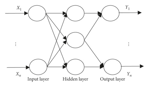
RBFNN is an artificial neural network which can approximate any nonlinear complex continuous function with any accuracy. It has the advantage of fast convergence speed and unique optimal approximation [14], which can solve the problem of local minimum. The basic structure of RBFNN is shown in Figure 1, which consists of input layer, hidden layer, and output layer.

Details are in the caption following the image — **Figure 1**
Open in figure viewer PowerPoint

Structure diagram of RBFNN.

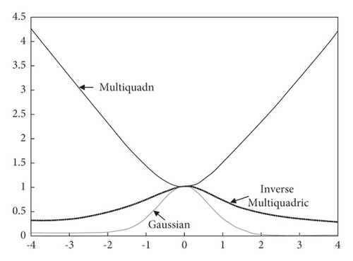
The common radial basis functions of RBFNN mainly include kernel functions, namely, Gaussian, multiquadric, and inverse multiquadric, and their radial basis function distribution is shown in Figure 2 [15]. It can be seen that, with the increase of center distance, multiquadric is a monotonically increasing function, while Gaussian and inverse multiquadric are monotonically decreasing functions. For monotonically decreasing function, when the variable is close to the function center, the function can obtain a large value; otherwise, its value tends to 0. Therefore, monotonically decreasing function has good local characteristics [16]. Thus, when RBFNN basis function is selected, monotonically decreasing function is usually used. Gaussian functions are characterized by simple form and good resolution [17]. Therefore, based on the advantages of Gaussian function, this paper uses it as the base function of RBFNN.

The basis function of Gaussian-RBFNN model can be expressed as [18]

\begin{matrix} φ_{i} (x) = \exp [\frac{- {‖X - e_{i}‖}^{2}}{2 σ_{i}^{2}}], i = 1,2, \dots m, \end{matrix}

(1)

where φ_i(x) is the output of hidden layer node i and

X = {(x_{1}, x_{2}, \dots, x_{n})}^{T}

is the input sample. The Gaussian function center of node i is e_i, and its variable is σ_i, namely, the base width.

The output of RBFNN is the linear combination of node output in the hidden layer [19]:

\begin{matrix} y_{k} = \sum_{i = 1}^{m} w_{i k} φ_{i} (x), k = 1,2, \dots, p, \end{matrix}

(2)

where w is the weight.

3. Nonlinear Complex Function Approximation Based on Gaussian-RBFNN

3.1. Multidimensional Gaussian-RBFNN Interpolation Approximation

The dataset is defined as (x_i, f_i), x_i ∈ [a, b]^k, f_i ∈ R, i − 0,1, …, n. Multidimensional Gaussian-RBFNN is W_a(x, A), and accurate Gaussian-RBFNN is W_e(x, A). The only difference between the two is the external weights, which can be expressed as

\begin{matrix} W_{a} (x, A) = \sum_{j - 0}^{n} f_{j} ϕ (A ‖x - x_{j}‖), \\ W_{e} (x, A) = \sum_{j = 0}^{n} k_{j} ϕ (A ‖x - x_{j}‖) . \end{matrix}

(3)

When A is large enough, W_a(x, A) can approximate W_e(x, A), and approximate dataset (x_i, f_i) ∈ R^R+1, i = 0,1, …, n.

Theorem 1. When i ≠ j and x_i ≠ x_j, dataset (x_i, f_i), x_i ∈ [a, b]^k, f_i ∈ R, i = 0,1, …, n, can determine W_e(x, A) and W_a(x, A). For any ε > 0 and x ∈ [a, b]^k, when a sufficiently large positive real variable A^′(A > A^′) is existing, there is

\begin{matrix} |W_{e} (x, A) - W_{a} (x, A)| < ε . \end{matrix}

(4)

Prove that W_e(x, A) exists:

\begin{matrix} k - f = k - M k = (I - M) k = (I - M) (k - f) + (I - M) f, \end{matrix}

(5)

where

k = {(k_{0}, k_{1}, \dots k_{n})}^{T}

represents the external weight, I represents the identity matrix, and M represents the matrix. Therefore,

\begin{matrix} {‖k - f‖}_{1} \leq \frac{{‖I - M‖}_{1}}{1 - {‖I - M‖}_{1}} {‖f‖}_{1}, \\ {‖I - M‖}_{1} = \max_{0 \leq j \leq n} \sum_{i \neq j} |m_{i j}| . \end{matrix}

(6)

According to Lemma 1 [20, 21], when ϕ(0) = 1, ϕ(x) is a monotonically decreasing function on interval |0, +∞|, and there is

\begin{matrix} |ϕ (x)| < 1, \\ Due to \underset{A ⟶ \infty}{Lim m_{i j}} = \underset{A ⟶ \infty}{Lim} ϕ (A ‖x - x_{j}‖) = 0, (i \neq j) . \end{matrix}

(7)

Therefore, in m_ij(i ≠ j), if ∀ε > 0, there is

\begin{matrix} ε^{'} = \min \{\frac{1}{(n + 1) (ε + {‖f‖}_{1})} ε, \frac{1}{n + 1}\} . \end{matrix}

(8)

Thus, A_ij > 0 is existing, and when A > A_ij, there is

\begin{matrix} |m_{i j}| < ε^{'} = \min \{\frac{1}{(n + 1) (ε + {‖f‖}_{1})} ε, \frac{1}{n + 1}\} . \end{matrix}

(9)

Therefore, when $A > A_{1} = max_{i \neq j} \{A_{i j}, i, j = 0,1, \dots, n\}$ , there is

\begin{matrix} {‖I - M‖}_{1} < n \cdot |m_{i j}| < \min \{\frac{1}{ε + {‖f‖}_{1}}, 1\} . \end{matrix}

(10)

Considering that f(x) = x/1 − x is a monotonically increasing function on interval (−∞, 1) [22], there are

\begin{matrix} {‖k - f‖}_{1} \leq \frac{{‖I - M‖}_{1}}{1 - {‖I - M‖}_{1}} {‖f‖}_{1} < \frac{ε / ε + {‖f‖}_{1}}{1 - (ε / ε + {‖f‖}_{1})} {‖f‖}_{1} < ε, \\ |W_{e} (x, A) - W_{a} (x, A)| = |\sum_{i = 0}^{n} (k_{i} - f_{i}) ϕ (A ‖x - x_{j}‖)| \leq {‖k - f‖}_{1} < ε . \end{matrix}

(11)

Therefore, it can be inferred that when i ≠ j and x_i ≠ x_j, the dataset (x_i, f_i), x_i ∈ [a, b]^k, f_i ∈ R, i = 0,1, …, n, determines W_a(x, A) and W_e(x, A). If ∀ε > 0, there is a sufficiently large positive real number A^′. When A > A^′, |f_i − W_a(x, A)| < ε.

3.2. Gaussian-RBFNN Approximating Nonlinear Complex Function

Based on the above analysis, Gaussian-RBFNN is used to approximate the nonlinear complex function. The specific process is as follows:

(1)
From 0 to 5, the nonlinear complex function is sampled every 0.1.
(2)
Calculate the sample function value and establish the Gaussian-RBFNN model.
(3)
The sample sets are divided into training sample set and testing sample set. The training sample set is adopted to train the model until the error is less than the set threshold or no longer changes, and the model is saved. After the training reaches the maximum number of iterations, if the error of the model is still greater than the set threshold or tends to decrease, the network structure of the model is adjusted, such as number of hidden layers and number of hidden layers’ neurons, and training continues until the requirements are met.

The newrb is used to construct a three-layer Gaussian-RBFNN. The used statements are as follows:

\begin{matrix} netl = newrb (p, t,goal,spread), \\ net 2 = newff (minmax (p), [n,1], \{‘ tansig ’, ’ purelin\}, ’ trainlm ’) . \end{matrix}

(12)

In net1, p and t are input and output vectors, respectively, goal is the error square sum, and spread is the radial base walking constant. In net2, p is the input vector. Furthermore, n and tansig are the number of hidden layer nodes and transfer function, respectively, purelin is the transfer function of the output layer, and trainlm is the adopted learning algorithm.

4. Simulation Experiment

4.1. Construction of Experimental Environment

This experiment uses the neural network toolbox developed under MATLAB7.0 environment to establish the simulation experiment of nonlinear complex function approximation. The experiment is carried out on 64-bit Windows7 operating system with Centrino2D 2.1ghz CPU, Tesla K80 GPU, and 16G memory.

4.2. Data Sources and Preprocessing

In this experiment, single-variable nonlinear function y = 7sin³x+0.2 × ²+4.5, x ∈ [0,5], is selected for simulation, and its function image is shown in Figure 3 [23]. In addition, the binary nonlinear function is

\begin{matrix} f_{2} (x, y) = x^{2} + y^{2} - 1020. (\cos 22 π x + \cos π y) + \end{matrix}

(13)

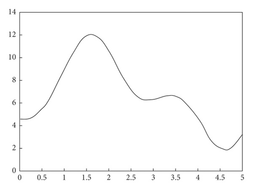
The nonlinear function is to be approximated.

4.3. Parameter Settings

Set the activation function of the proposed model as $ϕ (x) = e^{- x^{2}}$ .

Define S = {(x, y) : −1 ≤ x ≤ 1, −1 ≤ y ≤ 1}, and it satisfies

\begin{matrix} n_{1} = 10^{2}, \\ A (100) = 8, \\ n_{2} = 20^{2}, \\ A (400) = 20, \\ n_{3} = 30^{2}, \\ A (900) = 40, \end{matrix}

(14)

where A(n) is the time parameter of model training.

4.4. Evaluation Indexes

Average training time, training standard error, RATT, RATR, and TRMSE are also adopted to evaluate the model performance, and the calculation methods are as follows [24–26]:

\begin{matrix} RATT = \frac{average training time of the proposed algorithm}{average training time of Gaussian - RBFNN}, \\ RATR = \frac{average testing RMSE of the proposed algorithm}{average testing RMSE of Gaussian - RBFNN}, \\ TRMSE = \sqrt{\frac{1}{n + 1} \sum_{i = 0}^{n} {(f (x_{i}, y_{i}) + W_{a} (x_{i}, y_{i}, A))}^{2}} . \end{matrix}

(15)

4.5. Experimental Results

4.5.1. Results of Single-Variable Nonlinear Function Approximation

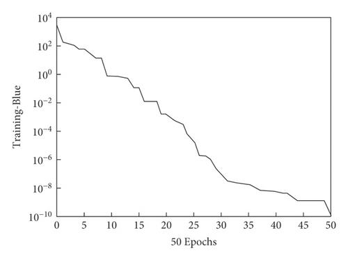
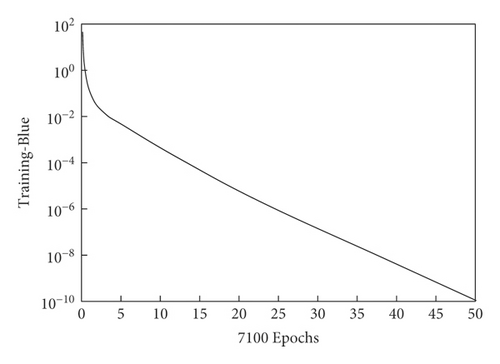
(1) Convergence Speed. The training processes of the proposed model and the BP neural network model approximating single-variable nonlinear function y = 7sin³x+0.2 × ²+4.5 are shown in Figure 4. The proposed model only needs 50 steps to complete training. However, the BP neural network model needs 7100 steps. In addition, the accuracy is slightly higher than that of the BP neural network model. Thus, the proposed model has certain advantages, and its convergence speed of nonlinear functions approximation is better than the current BP network model.

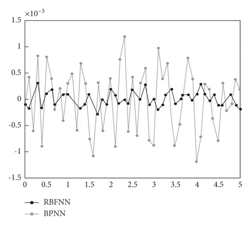
(2) Approximation Ability. The comparison of errors in the training process of the proposed model and the BP model is shown in Figure 5, where the simulation error of the proposed model is close to 0, and the oscillation amplitude of the simulation error of the BP neural network model is significantly higher than that of the proposed model. Furthermore, the approximation accuracy of two models to training samples is 10⁻³. Thus, the proposed model has better approximation ability to training samples, almost reaching complete approximation.

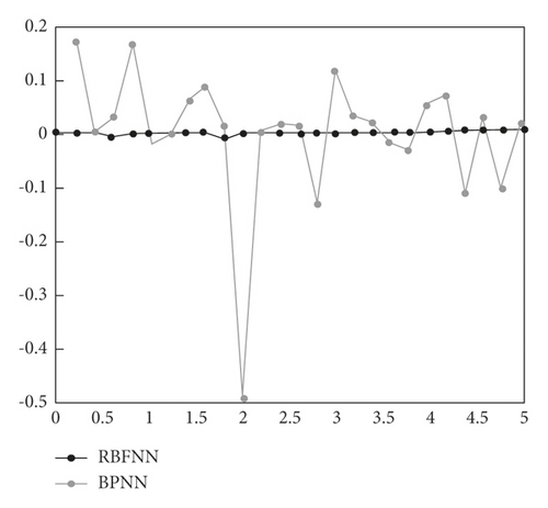
The proposed model and the BP neural network model approximate nontraining samples, and the comparison of errors are shown in Figure 6. Compared with the BP neural network model, the proposed model has significantly better approximation ability to the nontraining samples, almost complete approximation. And the overall simulation error is less than 0.1. However, the BP neural network model has a large error fluctuation, and the maximum error is close to 0.5. This shows that the proposed model has better approximation ability to nontraining samples.

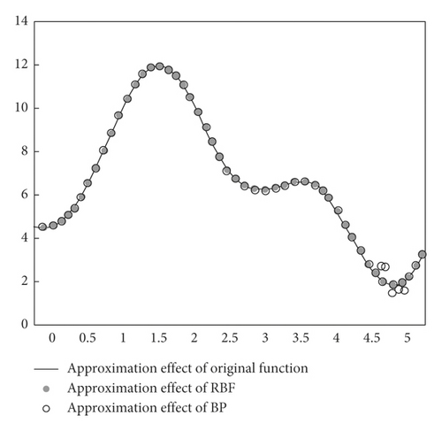
The proposed model and the BP model are used to overall approximate y = 7sin³x+0.2 × ²+4.5, and the results are shown in Figure 7. Here, the proposed model is entirely consistent with y = 7sin³x+0.2 × ²+4.5. However, the BP model is inconsistent with some function segments of y = 7sin³x+0.2 × ²+4.5. Therefore, the overall approximation of the proposed model is better than that of the BP neural network model, and the overall effect is great.

(3) Network Structure. The number of hidden layer neurons is a main index to measure the complexity of the network structure. To compare the network structure of the proposed model and the BP neural network model, different training sample numbers are used to construct the proposed model and its comparison model, and the number of neurons of the proposed model and the comparison model is shown in Table 1. Here, under the same number of training samples, the number of hidden layer neurons of the proposed model is higher than that of the BP neural network model. It means that when training the same samples, the network structure of the proposed model is more complex than that of the BP neural network model.

Table 1. Comparison of parameter settings for different methods.

Sample number	RBF neuron number	BP neuron number
21	21	13
35	35	24
41	41	20
67	67	22
85	88	35

Therefore, the proposed model can well approximate the single-variable nonlinear function with high approximation accuracy, and the overall approximation error is less than 0.1.

4.5.2. Approximation Results of Binary Nonlinear Functions

Figure 8 shows the uniform approximation results of the proposed model to the binary nonlinear function f₂(x, y) = x² + y² − 10(cos 2 πx + cos 2 πy) + 20. Figure 9 shows the relationship between A and n and TRMSE when the proposed model approximates f₂(x, y) = x² + y² − 10(cos 2 πx + cos 2 πy) + 20. The proposed model has a good approximation effect for binary nonlinear complex function f₂(x, y) = x² + y² − 10(cos 2 πx + cos 2 πy) + 20. With the increase of A and n, the model will uniformly converge to f₂(x, y).

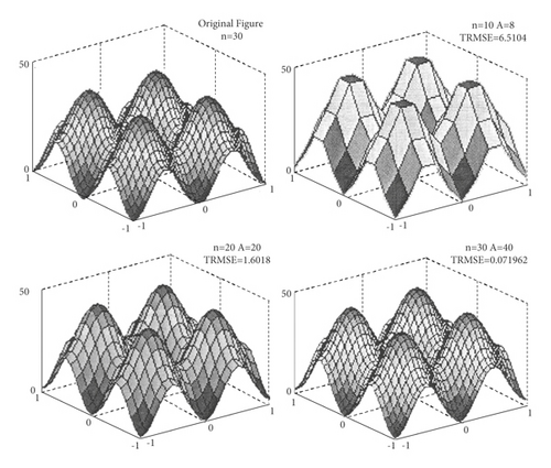
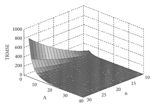
Table 2 shows the comparison of approximation performance of the proposed model and BP neural network to binary nonlinear complex function f₂(x, y) = x² + y² − 10(cos 2 πx + cos 2 πy) + 20. The performance of the proposed model is better than that of the BP neural network model on average training time, training standard error, RATT, RATR, and TRMSE, which indicates that the proposed model has better approximation performance.

Table 2. Performance comparison of different models.

Performance	Training		Test				Parameter
Performance	Time	RATT	Time	TRMSE	Dev	RATR	n = 20
RBFNN	0.11875	1	0.115625	0.00375471	0	1	A = 40
BPNN	1.095313	9.223684	0.010938	0.07008864	0.04897677	18.66685	Node = 60

5. Application Analysis of the Gaussian-RBFNN Model

5.1. Data Source and Preprocessing

For the verification of the practical application effect of the proposed method, it is used to approximate stock price to predict the stock price. The Shanghai composite index of 300 consecutive trading days from April 1, 2018, to September 6, 2019, is selected as the experimental sample, the closing price is used as the prediction object, and the prediction period is 5 days [27]. In addition, datasets are divided into the training set and the testing set. There are 290 data in the training set and 10 data in the testing set.

To make the data samples meet the input and output requirements of the Gaussian-RBFNN model, before model prediction, premnmx and postmnmx functions in MATLAB7.0 are called to perform normalization and inverse normalization for the input and output models, respectively. The normalized data format of premnmx is shown in formula (16), and the reverse-normalized data format of postmnmx is shown in formula (17) [28, 29]:

\begin{matrix} [p_{n}, \min p, \max p, t_{π}, \min t, \max t] = premmmx (P, T), \end{matrix}

(16)

\begin{matrix} [P, T] = postmnmx (p_{n}, \min p, \max p, t_{π}, \min t, \max t), \end{matrix}

(17)

where P is the input data, minp and maxp are the minimum and maximum values of P, T is the output data, and mint and maxt are the minimum and maximum values of T.

5.2. Construction of the Stock Prediction Model

We use the newrb function in MATLAB7.0 to build the Gaussian-RBFNN model and train it automatically, and its format is shown as

\begin{matrix} Net = newrv (p, t, goal, sperad), \end{matrix}

(18)

where p and t represent the input and output vectors of the model, respectively. With five days as a positive cycle, the Shanghai composite index from the first day to the fifth day is used to predict the Shanghai composite index of the sixth day, the Shanghai composite index from the second day to the sixth day is used to predict the Shanghai composite index of the seventh day, and so on. On the one hand, the closing prices of 226–279 trading days are constructed as a 5∗50 matrix, and the matrix is used as the input vector of model. On the other hand, the closing prices of 231–280 trading days are constructed as a 1∗50 matrix, and the matrix is used as the output vector of model. Then, y1 = sim(net, p1) is utilized for fitting prediction.

5.3. Results and Analysis

5.3.1. Analysis of Prediction Accuracy

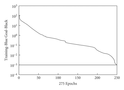
Figure 10 shows the trend of training errors when the proposed model predicts stock prices. The training error of the proposed model is less than 0.1, which realizes the required prediction accuracy. The model completes the training through 275 steps, which means that the convergence speed of model is fast. Therefore, the prediction accuracy and convergence speed of the proposed model are effective.

5.3.2. Comparison of Prediction Effects

The effectiveness of the proposed method in practical application is further verified by comparing prediction results on the closing price of the stock exchange index for 50 trading days from June 29, 2018, to September 6, 2018. The results are shown in Figure 11. Compared with the comparison model, the predicted value of the proposed model is closer to the actual value, and the fitting effect of the predicted value curve and the actual value curve is better. Thus, the proposed model has higher prediction accuracy and better prediction effect.

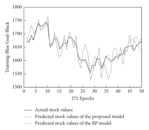
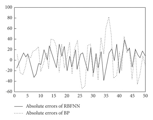
Figure 12 shows the comparison of absolute errors of the proposed model and BP neural network model predicting the closing price of Shanghai composite index in 50 trading days from June 29, 2020, to September 6, 2020. Here, the prediction absolute error of the proposed model has a small fluctuation range. There are about 72% absolute error values concentrated on interval [-20, 20], and the maximum error is less than ±40, which basically achieves the ideal prediction effect. However, the fluctuation range for absolute error of the BP neural network model is larger, which mainly focuses between [-40,-20] and [20,40], accounting for 48% of the total. In addition, there are a few absolute errors between [-60,-40] and [40,60], and one absolute error exceeds 80, which means that its prediction effect is poor. Thus, the proposed model has certain effectiveness and superiority in practical application.

6. Conclusion

To sum up, the proposed Gaussian-RBFNN model can approximate single-variable nonlinear complex functions and binary nonlinear complex functions, and the approximation effect is good. Compared with the BP neural network model, the proposed model performs better in average training time, training standard error, RATT, RATR, and TRMSE. In addition, the training speed of the proposed model is faster, and the approximation effect is better. The approximation error is less than 0.1, which can achieve the ideal approximation effect. In practical stock prediction application, the proposed model has good curve fitting effect of the predicted value and the actual value, and the training absolute error is less than 0.1, which can achieve the required prediction accuracy. Compared with the BP neural network model, the proposed model has certain advantages and precision in prediction accuracy and convergence speed. Moreover, a new idea and reference are provided for deep learning in the analysis of nonlinear complex function problems. As can be seen, some research achievements have been obtained in this paper, but because of the limitations of conditions, there are still some shortcomings to be improved. Here, only the Gaussian-RBFNN model is studied, and the prediction effect of the RBFNN model with other base function is not considered. Therefore, the next research is to find an optimal nonlinear complex function approximation method by deeply exploring this aspect.

Conflicts of Interest

The authors declare that they have no conflicts of interest regarding this work.

Open Research

Data Availability

The experimental data used to support the findings of this study are available from the corresponding author upon request.

References

1 Mantovani R. G., Rossi A. L. D., Alcobaça E., Vanschoren J., and de Carvalho A. C. P. L. F., A meta-learning recommender system for hyperparameter tuning: predicting when tuning improves SVM classifiers, Information Sciences. (2019) 501, 193–221, https://doi.org/10.1016/j.ins.2019.06.005, 2-s2.0-85067004352.
10.1016/j.ins.2019.06.005
Web of Science® Google Scholar
2 Jia X., Guo Y., Zhao B., and Huang Y., Fractional-integral-operator-based improved SVM for filtering salt-and-pepper noise, IET Image Processing. (2019) 13, no. 12, 2346–2357, https://doi.org/10.1049/iet-ipr.2019.0624, 2-s2.0-85073693072.
10.1049/iet-ipr.2019.0624
Web of Science® Google Scholar
3 Xu Y., Huang Y., and Ma G., A beetle antennae search improved BP neural network model for predicting multi-factor-based gas explosion pressures, Journal of Loss Prevention in the Process Industries. (2020) 65, 104117–104127, https://doi.org/10.1016/j.jlp.2020.104117.
10.1016/j.jlp.2020.104117
Web of Science® Google Scholar
4 Chen X., Meng X., and Zhao Y., Genetic algorithm to improve Back Propagation Neural Network ship track prediction, Journal of Physics: Conference Series. (2020) 1650, no. 3, 032133–032139, https://doi.org/10.1088/1742-6596/1650/3/032133.
10.1088/1742-6596/1650/3/032133
Google Scholar
5 Lou Y., Xing Y., Li X., and Xu S., A new approach of CMT seam welding deformation forecasting based on GA-BPNN, Frattura Ed Integrità Strutturale. (2020) 14, no. 53, 325–336, https://doi.org/10.3221/igf-esis.53.25.
10.3221/IGF-ESIS.53.25
Google Scholar
6 Razaque A., Ben Haj Frej M., Almi’ani M., Alotaibi M., and Alotaibi B., Improved support vector machine enabled radial basis function and linear variants for remote sensing image classification, Sensors. (2021) 21, no. 13, 4431–4438, https://doi.org/10.3390/s21134431.
10.3390/s21134431
Web of Science® Google Scholar
7 Zhang X. and Wang M., Improved SVM classification algorithm based on KFCM and LDA, Journal of Physics: Conference Series. (2020) 1693, no. 1, 012107–012110, https://doi.org/10.1088/1742-6596/1693/1/012107.
10.1088/1742-6596/1693/1/012107
Google Scholar
8 Ma T.-b., Qing Z., Fei D., and Jian L., Fault diagnosis of piezoelectric sensor patches for vibration control based on multifeature fusion and improved SVM, Shock and Vibration. (2019) 2019, 1–16, https://doi.org/10.1155/2019/8239198.
10.1155/2019/8239198
Web of Science® Google Scholar
9 Huang W., Oh S. K., and Pedrycz W., Fuzzy reinforced polynomial neural networks constructed with the aid of PNN architecture and fuzzy hybrid predictor based on nonlinear function, Neurocomputing. (2021) 458, 454–467, https://doi.org/10.1016/j.neucom.2021.06.047.
10.1016/j.neucom.2021.06.047
Web of Science® Google Scholar
10 Ramandeep B., Derivative-free king’s scheme for multiple zeros of nonlinear functions, Mathematics. (2021) 9, no. 11, https://doi.org/10.3390/math9111242.
10.3390/math9111242
Web of Science® Google Scholar
11 Karami H., Mobayen S., Lashkari M., Bayat F., and Chang A., LMI-Observer-Based stabilizer for chaotic systems in the existence of a nonlinear function and perturbation, Mathematics. (2021) 9, no. 10, https://doi.org/10.3390/math9101128.
10.3390/math9101128
Web of Science® Google Scholar
12 Aliskan I., Optimized inverse nonlinear function-based wiener model predictive control for nonlinear systems, Arabian Journal for Science and Engineering. (2021) 46, 10217–10230.
10.1007/s13369-021-05681-w
Web of Science® Google Scholar
13 Dai J., Li Y., Xiao L., Jia L., Liao Q., and Li J., Comprehensive study on complex-valued ZNN models activated by novel nonlinear functions for dynamic complex linear equations, Information Sciences. (2021) 561, 101–114, https://doi.org/10.1016/j.ins.2020.12.078.
10.1016/j.ins.2020.12.078
Web of Science® Google Scholar
14 Syah R., Ahmadian N., Elveny M., Alizadeh S. M., Hosseini M., and Khan A., Implementation of artificial intelligence and support vector machine learning to estimate the drilling fluid density in high-pressure high-temperature wells, Energy Reports. (2021) 7, 4106–4113, https://doi.org/10.1016/j.egyr.2021.06.092.
10.1016/j.egyr.2021.06.092
Web of Science® Google Scholar
15 Zheng H., Wu M. X., Shi Y., Deng C., and Zhang C. Z., 3D elastic dental analysis by a local RBF collocation method, Applied Mathematical Modelling. (2021) 99, 41–56, https://doi.org/10.1016/j.apm.2021.06.015.
10.1016/j.apm.2021.06.015
Web of Science® Google Scholar
16 Zhang J. and Zeng X., Multi-touch gesture recognition of braille input based on petri net and RBF net, Multimedia Tools and Applications. (2021) 78, 1–19.
Google Scholar
17 Wu Ye and Sun X., Optimization and simulation of enterprise management resource scheduling based on the radial basis function (RBF) neural network, Computational Intelligence and Neuroscience. (2021) 2021, 6025492–6025498, https://doi.org/10.1155/2021/6025492.
10.1155/2021/6025492
PubMed Web of Science® Google Scholar
18 Liu C.-Y., Ku C.-Y., Hong L.-D., and Hsu S.-M., Infinitely smooth polyharmonic RBF collocation method for numerical solution of elliptic PDEs, Mathematics. (2021) 9, no. 13, https://doi.org/10.3390/math9131535.
10.3390/math9131535
Web of Science® Google Scholar
19 Wang B., Jahanshahi H., Volos C., Bekiros S., Khan M. A., Agarwal P., and Aly A. A., A new RBF neural network-based fault-tolerant active control for fractional time-delayed systems, Electronics. (2021) 10, no. 12, 1501–1508, https://doi.org/10.3390/electronics10121501.
10.3390/electronics10121501
Web of Science® Google Scholar
20 Wang S., Yin X., Li P., Zhang Y., Wang X., and Tong S., Cognitive control using adaptive RBF neural networks and reinforcement learning for networked control system subject to time-varying delay and packet losses, Arabian Journal for Science and Engineering. (2021) 63, 1–15, https://doi.org/10.1007/s13369-021-05752-y.
10.1007/s13369-021-05752-y
Google Scholar
21 Yu C., Wang Y., Zhang H., Gao B., and He Y., Thermal-hydraulic performance prediction of two new heat exchangers using RBF based on different DOE, Open Physics. (2021) 19, no. 1, 285–304, https://doi.org/10.1515/phys-2021-0017.
10.1515/phys-2021-0017
Web of Science® Google Scholar
22 Yang Y., Luo J., Huang Q., Wu W., and Sun Y., Weighted double-logistic function fitting method for reconstructing the high-quality sentinel-2 NDVI time series data set, Remote Sensing. (2019) 11, no. 20, 2342–2352, https://doi.org/10.3390/rs11202342, 2-s2.0-85074203869.
10.3390/rs11202342
Web of Science® Google Scholar
23 Torabi A., An efficient plasmonic waveguide mode solution using rational function fitting of Green's function, Optical Review. (2019) 26, no. 2, 278–282, https://doi.org/10.1007/s10043-019-00498-3, 2-s2.0-85061695454.
10.1007/s10043-019-00498-3
CAS Web of Science® Google Scholar
24 Zhang Y., Niu J., and Na S., A novel nonlinear function fitting model based on FOA and GRNN, Mathematical Problems in Engineering. (2019) 2019, 10, 2697317, https://doi.org/10.1155/2019/2697317, 2-s2.0-85062327656.
10.1155/2019/2697317
Web of Science® Google Scholar
25 Cao B., Li H., Cai E., and Fan M., Determination of pesticides in flour by terahertz time-domain spectroscopy (THz-TDS) with voigt function fitting and partial least squares (PLS) analysis, Analytical Letters. (2020) 69, 1–12.
Google Scholar
26 Huo Y., Hu W., Li Z., and Rao Z., Research on parameter identification and state of charge estimation of improved equivalent circuit model of Li-ion battery based on temperature effects for battery thermal management, International Journal of Energy Research. (2020) 44, no. 14, 11583–11596, https://doi.org/10.1002/er.5784.
10.1002/er.5784
CAS Web of Science® Google Scholar
27 Long C., Wen-k S., Song L., Zhi-yong C., and Yuan-bin Y., Modeling of multistage nonlinear Dual Mass Flywheel torsional damper based on smoothing function fitting, Proceedings of the Institution of Mechanical Engineers - Part D: Journal of Automobile Engineering. (2021) 235, no. 1, 32–42, https://doi.org/10.1177/0954407020951318.
10.1177/0954407020951318
Web of Science® Google Scholar
28 Goldberg N., Rebennack S., Kim Y., Krasko V., and Leyffer S., MINLP formulations for continuous piecewise linear function fitting, Computational Optimization and Applications. (2021) 63, 1–11, https://doi.org/10.1007/s10589-021-00268-5.
10.1007/s10589-021-00268-5
Google Scholar
29 Cao B., Li H., Cai E., and Fan M., Determination of pesticides in flour by terahertz time-domain spectroscopy (THz-TDS) with voigt function fitting and partial least squares (PLS) analysis, Analytical Letters. (2021) 54, no. 5, 830–841, https://doi.org/10.1080/00032719.2020.1783676.
10.1080/00032719.2020.1783676
CAS Web of Science® Google Scholar

Citing Literature

All articles