In order to improve the effect of speech emotion research, this paper combines data mining technology to construct a speech emotion research model and establishes a state space model of speech emotion risk problem. Moreover, this paper uses fuzzy variables to describe the external uncertain environmental factors and intuitively shows the relationship between each technology, that is, clearly shows how actions and external environmental factors affect their action results, which is helpful in understanding the voice emotional risk problem from the root. In addition, this paper uses the basic knowledge of credibility theory to transform the model and finally transform the model into an optimal control problem. Through the speech emotion simulation experiment, it can be seen that the multilingual speech emotion analysis model based on data mining proposed in this paper has a good effect in speech emotion analysis.

1. Introduction

Discrete speech emotion recognition processes emotions into categories and this type of research suggests that there are several basic emotions in the brain. The most well-known classification criteria are six categories of emotions [1], including happy, sad, surprise, fear, anger, and disgust. However, scholars such as Baron-Cohen believe that cognitive mental states frequently occur in daily interactions, and they are not expressed through a few basic emotions. That is, a single sentiment label or limited discrete categories cannot adequately describe such complex sentiments. Therefore, some researchers consider replacing sentiment classification labels (namely, discrete sentiment) with continuous sentiment values (namely, dimensional sentiment) in multidimensional space [2].

Reference [3] proposes an emotional space description model consisting of Arousal (i.e., motivation, describing the intensity of emotion) and Valence (i.e., valence, describing the positive and negative degree of emotion). Among various continuous emotion space description models, the most abundant emotion description model is a four-dimensional space description model: Arousal-Valence-Power-Expectancy. Dimensional speech emotion recognition is a speech emotion research based on the emotion space description model. Dimensional discretization speech emotion recognition refers to using a transformation strategy to convert continuous emotion values in each dimension into a limited number of categories on the basis of dimension emotion annotation and then classify and recognize the converted emotion [4]. Reference [5] quantifies continuous labels in two dimensions of Valence-Arousal to four and seven classes and predicts the quantized sentiment labels on a conditional random domain model. The selection of speech emotion features is a crucial issue in speech emotion recognition [6]. Although the Low-level descriptors (LLD) features used in each corpus are not the same, for example, the LLD features related to energy, spectrum, and sound are used in the AVEC2012 corpus, while the LLD features in the IEMOCAP corpus mainly contain information related to energy, spectrum and fundamental frequency [7]. These LLD features contain rich emotional information and also lead to a sharp increase in the number of features, which are basically between 1000 and 2000. Too many features will bring information redundancy to a certain extent, and the dependencies between features may also be uncontrollable, which will greatly hinder the training of emotion recognition models [8]. Subsequently, some researchers began to explore some high-level features of knowledge-based features. Research results have shown that knowledge-based features may be more predictive of emotion recognition [9]. Reference [10] proposed to use a disfluency feature and nonverbal feature (Disfluency and Non-verbal, DIS-NV) to identify the emotion in the dialogue and obtained a relatively good recognition accuracy. Another essential part of speech emotion recognition is the selection of recognition models. These models can achieve a good result in emotion recognition performance, but these models ignore the temporal information in emotion features [11]. In comparison, Long Short Term Memory Recurrent Neural Network (LSTM-RNN) can learn long-distance dependency information of features [12]. That is, the LSTM model is more suitable for long-distance information modeling in emotion recognition. Studies have shown that long short-term memory networks [13].

Since the introduction of deep learning, many researchers have begun to make breakthroughs [14]. People attribute deep learning problems to three elements: data, algorithms, and computing power [15]. Computing power refers to the environmental problems required for deep learning, mainly referring to the computing power of computers. GPU has powerful floating-point computing capabilities and efficient parallel computing capabilities, especially for tasks requiring high-density computing such as image processing, which provides strong support for accelerating deep learning operations. Algorithms refer to various methods of deep learning, and algorithms are inseparable from the support of data. The data determines the upper limit of the algorithm, and the algorithm is just constantly approaching this upper limit [16]. Given the importance of data to algorithms, some organizations have begun to build high-quality datasets around their research directions or commercial application purposes.

The public multimodal datasets are mainly used for facial expression recognition, image description, visual question answering, object and scene detection and recognition, and semantic segmentation. These datasets have not paid much attention to the problem of discrimination. Most of the datasets are too coarse-grained for the classification of emotional issues and almost do not contain expressions related to discrimination. Some expression recognition datasets, such as the RaFD dataset, contain categories related to discrimination. The RaFD dataset categorizes expressions into 8 expressions . This facial discrimination expression is too obvious and the modalities are single, and other types of discrimination such as various gesture discrimination and implicit discrimination in some specific scenarios cannot be effectively studied [17]. The multimodal high-level semantic-oriented discrimination studied in the literature [18] is mostly implicit discrimination in specific scenarios, and the image and text alone do not convey any discriminatory emotion, and when the two appear together, they will express discrimination emotion. This kind of discrimination constitutes a complex condition, and the currently published datasets have not conducted in-depth research on this issue, and this multimodal high-level semantic discrimination problem may have an early adverse impact on an individual’s mental health and social stability. Manual detection of this problem: The problem of this kind of discrimination will consume huge resources, so it is very necessary to establish a high-quality dataset for this problem and make a little contribution to the study of multimodal discrimination. The discrimination-oriented multimodal dataset constructed in [19] focuses on the high-level semantics of images and texts and also studies gestures with obvious discrimination information. There are many kinds of gesture discrimination, which can be roughly summarized as pointing discrimination and face-to-face discrimination in terms of the positional relationship.

In order to improve the effect of speech emotion analysis, this paper combines data mining technology to build a speech emotion research model to improve the effect of speech emotion analysis.

2. Speech Emotion Recognition Algorithm

2.1. Expected Value of Fuzzy Variable Function

Definition 1. If it is assumed that ζ is a fuzzy variable defined on the credibility space (Θ, P(Θ), Cr), and f : ℜ⟶ℜ is a mapping to a real number set, the expected value E[f(ζ)] of the function is defined as follows:

(1)

Among them, at least one integral in the above formula is finite.

We assume that ζ is a fuzzy variable on the credibility space (Θ, P(Θ), Cr), and its credibility density function ϕ(x) and credibility distribution Φ(x) both exist. If the Lebesgue integrals and are finite, there is the following:

(2)

2.2. Parametric Model of Emotional Risk in Fuzzy Environment

In order to introduce the emotional risk model of hidden actions more clearly, we use Figure 1 to describe the emotional risk game sequence of hidden actions, which is helpful for the following understanding.

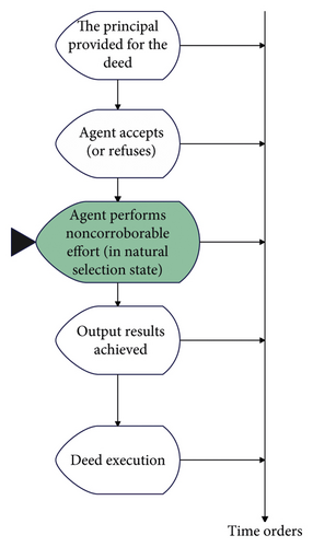
Details are in the caption following the image — Open in figure viewer PowerPoint

In previous studies, random variables are often used to represent the external uncertain environmental factors.

Before the principal’s expected utility maximization model is established, in order to more clearly describe the emotional risk problem in the fuzzy environment, the notation and assumptions used in this chapter are firstly given.

The basic assumptions are as follows:

2.2.1. Symbol

e, is the effort level of the agent;
ψ(e), is the cost at which the agent’s effort level is e;
q, is the performance of the agent, that is the output;
Φ(x, e), is the reliability distribution function of q when the effort level is e;
ϕ(x, e), is the confidence density function of q when the effort level is e;
t(q), is the emotional output that the agent receives from the principal;
U(t), is the utility function of the agent for the emotional output t;
S(q), is the income function of the principal is the income brought by the output of q unit of the agent to the principal;
V(S), is the principal’s utility function for revenue.

2.2.2. Assumptions

(1)
The output q is a fuzzy variable whose support is Ω = [a, b], and its credibility density function satisfies ∂²ϕ(x, e)/∂e² ≤ 0.
(2)
The emotional output t(x) is monotonically increasing with respect to x, that is, dt(x)/dx ≥ 0. Moreover, there is a large positive number M that allows us to obtain 0 ≤ dt(x)/dx ≤ M, that is, M is the upper bound of dt(x)/dx, which means that the rate of change of the emotional output is lower than a certain level. That is to say, the rate of change of the acceptable emotional output set by the entrusted input is lower than a certain value. Obviously, this assumption is completely in line with the actual situation.
(3)
The client’s revenue function S(x) satisfies dS(x)/dx > 0, d²S(x)/dx² ≤ 0, and there is S(0) = 0:
(4)
The utility function of the principal is V(S(x)) − t(x), and we set dV(S(x))/dx ≥ dt(x)/dx; that is, for the unit change of the output q, the rate of change of the principal’s utility for this part of the income is larger than the rate of change of the emotional output.
(5)
The cost function of the agent's effort satisfies ψ(e) ≥ 0, dψ(e)/de > 0 and d²ψ(e)/de² > 0, which indicates that as the effort level increases, the cost to be paid increases. At the same time, as the effort level increases, the cost required to improve the unit effort level, that is, the marginal cost also increases.
(6)
The utility function of the agent is U(t(q)) − ψ(e). Among them, U(⋅) satisfies dU(t)/dt > 0, d²U(t)/dt² ≤ 0; that is, the agent uses a fuzzy variable to describe the agent’s output q, so the principal's utility V(S(q)) − t(q) is also a fuzzy variable. Therefore, the expected utility of the principal is as follows:
(3)

Strictly speaking, a contract that induces an agent to perform effort level e should satisfy: when the agent exerts effort level e, the utility he obtains will be greater than that obtained when he exerts any other level of effort. These constraints are called incentive compatibility constraints, which are expressed as follows:

(4)

Among them, refers to the set of all e^’ that maximize E[U(t(q))] − ψ(e^’).

In order to ensure that the agent is willing to participate in this contractual relationship and successfully complete the agency task, the level of utility brought to the agent by the contract provided by the principal cannot be lower than the level of utility that the agent can obtain when the latter does not participate in the contractual relationship (called retain utility). These constraints are called the participation constraints of the agent. Here, for the convenience of analysis, it is usually assumed that the retained utility of the agent is zero, and the participation constraint can be expressed as follows:

(5)

In this game model, the principal takes action first. As the designer of the contract, he has the right to design the contract form that meets his own requirements. Here, the emotional output designed by the client should meet the following conditions: its rate of change should be limited within a certain range, that is,

(6)

The above formula indicates that the rate of change of emotional output must be greater than zero, but it must also be limited to a certain value and cannot increase without limit. This assumption is perfectly reasonable.

Definition 2. If a set of contracts satisfies both the incentive compatibility constraint and the participation constraint, that is, formulas (14) and (16), then the set of contracts is said to be incentive feasible.

Therefore, the principal’s expected utility maximization model can be established as follows:

(7)

2.3. Model Analysis and Solution

In this section, in order to find the optimal solution of model (16), we first analyze the principal’s objective function and the agent’s incentive compatibility constraints and participation constraints so as to give the equivalent form of model (16).

The client’s objective function can be written in the following form:

(8)

Proof. We only need to verify that V(S(x)) − t(x) is monotonically increasing with respect to x. According to dV(S(x))/dx − dt(x)/dx, we have the following:

(9)

That is, V(S(x)) − t(x) is monotonically increasing with respect to x. It can be obtained as follows:

(10)

The proof is complete.

The incentive compatibility constraint (14) can be transformed into the following form:

(11)

Proof. Since there is dU(t)/dt > 0 and dt(x)/dx ≥ 0, there is dU(t(x))/dx = dU(t)/dt · dt(x)/dx ≥ 0; that is, U(t(x)) is monotonically increasing with respect to x. It can be seen that

(12)

Furthermore, there is the following:

(13)

Therefore, the incentive compatibility condition can be transformed into the following form:

(14)

The incentive compatibility constraint (19) can be further transformed into the following:

(15)

Proof. First, we set

(16)

The first and second partial derivatives of L(t, e) with respect to e are calculated separately below:

(17)

and

(18)

According to ∂²ϕ(x, e)/∂e² ≤ 0 and d²ψ(e)/de² > 0, we can know ∂²L(t, e)/∂e² < 0, that is,

(19)

is a concave function of e. From the knowledge of calculus, it can be known that the maximum point of L(t, e) exists and is unique, and it makes the first-order partial derivative of L(t, e) with respect to e to be zero. Therefore, formula (19) can be transformed into the following:

(20)

Through the above analysis of the model, the incentive compatibility constraints and participation constraints are transformed into integral forms, and the following conclusions can be obtained.

Model (16) can be transformed into the following form:

(21)

The incentive compatibility constraint (19) is equivalent to the following:

(22)

Meanwhile, there is the following:

(23)

Among them, there is the following:

(24)

Proof. Because there is the following:

(25)

There is the following:

(26)

Moreover, there is the following:

(27)

The proof is complete.

The participation constraint (20) is equivalent to the following:

(28)

Meanwhile, there is the following:

(29)

Among them, there is the following:

(30)

Proof. Because there is the following:

(31)

There is the following:

(32)

Moreover, there is the following:

(33)

The proof is complete.

Model (21) can be transformed into an optimal control problem of the form:

(34)

Among them, Q(x), R(x) and t(x) are state variables, and v(x) is a control variable.

Through the above analysis, the emotional risk problem model in the principal-agent can be transformed into an optimal control problem. Among them, Q(x), R(x) and l(x) are state variables and v(x) is a control variable (refer to the literature). Therefore, the necessary conditions for the existence of the optimal solution of the model can be given by using the Pontryagin maximum principle (refer to the literature), and the specific solution steps are given.

First, the Hamiltonian function of model (45) can be defined as follows:

(35)

Among them, Q(x), R(x) and t(x) are state variables, v(x) is the control variable, λ, μ and γ are the corresponding costate variables.

The necessary conditions for the existence of optimal solutions can be obtained by applying the Pontryagin maximum principle. That is, if Q^∗, R^∗, t^∗ and v^∗ are the optimal solutions of the optimal control problem (45), there are optimal costate variables λ, μ and γ such that Q^∗, R^∗, t^∗, v^∗ and λ, μ, γ satisfy the following equations and boundary conditions.

(1)
Regular equation system
(36)
(2)
Boundary conditions
(37)
(3)
On [0, M], v^∗ maximizes the Hamiltonian function (24), that is,
(38)

Therefore, corresponding to the above problem, combined with the specific form of the Hamiltonian function, the expression of the necessary conditions for the existence of the optimal solution is given, and the following conclusions can be obtained.

The optimal solution (t^∗(q), e^∗) of the emotional risk model that maximizes the expected utility of the principal satisfies the following conditions:

(1)
Regular equation system
(39)
(2)
Boundary conditions
(40)
(3)
On [0, M], v^∗ maximizes the Hamiltonian function (45), that is,
(41)

For a special case, that is, the case where the utility function of the agent is a linear function; that is, the case of U(x) = kx, k > 0, the specific solution steps are discussed.

It can be known from the regular equation

(42)

Therefore, according to dλ(x)/dx = 0, dμ(x)/dx = 0 (that is, λ, μ is independent of x) and boundary condition λ(b) = 0, we have the following:

(43)

Among the specific problems, ϕ(x, e) is known, then we can find the specific expression of γ(x) . It is also known that on [0, M], v^∗ maximizes the Hamiltonian function (34), that is,

(44)

In the Hamiltonian function, there is only γ(x)v(x) which contains the control variable v(x), then v^∗ maximizes the Hamiltonian function, that is, v^∗ maximizes γ(x)v(x). Therefore, it is only necessary to specifically determine the switching point of v(x) according to the sign of γ(x), that is, when there is γ(x) > 0, there is v^∗x = M. When there is γ(x) < 0, there is v^∗x = 0. Finally, combined with the boundary conditions of dt(x)/dx = v(x) and t(x), the specific expression of the emotional output t^∗(x) can be given. Among them, λ, μ is determined by the boundary conditions. The above solution process is described below with a specific example.

We set V(S) = In(1 + S), S(x) = x, U(x) = kx, k > 0, ψ(e) = e²

It can be known from the regular equation

(45)

Therefore, according to condition dλ(x)/dx = 0, dμ(x)/dx = 0 (that is, λ, μ is independent of x) and boundary condition γ(+∞) = 0, we can get the following:

(46)

The cases are discussed in the following case by case.

Case 1. λ > 0

When there is x > (1 − kμ)e²/kλ + a, there is γ > 0, so there is v(x) = M. At this point, there is t(x) = Mx + c₁

When there is x ≤ (1 − kμ)e²/kλ + a, there is γ ≤ 0, so there is v(x) = 0. At this point, there is t(x) = c₂. At the same time, because there is t(a) = 0, there is c₂ = 0, that is,

(47)

Among them, there is c₁ = −M[(1 − kμ)e²/kλ + a]

The expression of t^∗(x) is brought into the incentive compatibility constraint (3.7) to obtain the optimal effort level e^∗, which satisfies the following formula:

(48)

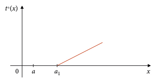
If we set , the optimal emotional output t^∗(x) is shown in Figure 2.

It can be seen that the optimal emotional output t^∗(x) is a piecewise function. That is, when the output result of the agent is below the limit value, it will not be able to obtain the emotional output. Only when the output result exceeds the limit value, can he obtain a positive emotional output. At this point, the sentiment output is a linear function with a growth rate of M.

Case 2. λ < 0

When there is x ≤ (1 − kμ)e²/kλ + a, there is γ ≥ 0, so there is v(x) = M. At this point, there is t(x) = Mx + c₃. At the same time, we know t(a) = 0, then there is t(x) = Mx − Ma.

When there is x > (1 − kμ)e²/kλ + a, there is γ < 0, so there is v(x) = 0. At this time, there is t(x) = c₄, that is,

(49)

Among them, there is. c₄ = M(1 − kμ)e²/kλ

The expression of l^∗(x) is brought into the incentive compatibility constraint (3.7) to obtain the optimal effort level e^∗, which satisfies the following formula:

(50)

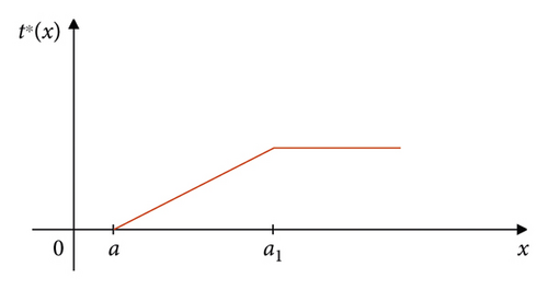
If we set , the optimal emotional output t^∗(x) is shown in Figure 3.

It can be seen from the figure that the optimal emotional output t^∗(x) is a piecewise function. The initial sentiment output is a linear function with a growth rate of M that increases as the output outcome increases. However, when the output result increases to a certain amount a₁, the emotional output will no longer increase, that is, maintain a fixed constant value. At this time, a certain number a₁ is large enough to ensure that the principal motivates the agent to make the optimal level of effort it is trying to motivate.

We set and output q as exponential fuzzy variables, and their membership functions are as follows:

(51)

The distribution function is as follows:

(52)

It can be known from the regular equation:

(53)

Therefore, according to dλ(x)/dx = 0, dμ(x)/dx = 0 (that is, λ, μ is independent of x) and boundary condition γ(+∞) = 0, we have the following:

(54)

The cases are discussed in the following case by case.

Case 3. λ < 0

When there is , there is γ ≥ 0, so there is v(x) = M. At this point, there is t(x) = Mx + m₁. At the same time, we know t(0) = 0, then there is t(x) = Mx.When there is , there is γ < 0, so there is v(x) = 0. At this time, there is t(x) = m₂. Among them, there is , that is,

(55)

Among them, there is .

The expression of t^∗(x) is substituted into the incentive compatibility constraint (19) to obtain the optimal effort level e^∗, which satisfies the following formula:

(56)

Case 4. λ > 0when there is , there is γ > 0, so there is v(x) = M. At this point, there is t(x) = Mx + m₃. Among them, there is .when there is , there is γ ≤ 0, so there is v(x) = 0. At this point, there is t(x) = m₄. At the same time, because there is t(0) = 0, there is m₄ = 0, that is,

(57)

Among them, there is .

The expression of t^∗(x) is brought into the incentive compatibility constraint (3.7) to obtain the optimal effort level e^∗, which satisfies the following formula:

(58)

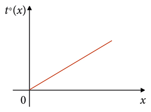
In particular, when there is λ > 0 and μ > 1/k, for any x, there is γ(x) > 0. At this point, there is v(x) = M, then there is t(x) = Mx + m₁. At the same time, because there is t(0) = 0, there is t^∗(x) = Mx. The optimal emotional output t^∗(x) is shown in Figure 4.

At this time, the optimal emotional output is a monotonically increasing linear function whose slope is the upper limit M of the rate of change of emotional output set by the client in advance.

The expression of t^∗(x) is brought into the incentive compatibility constraint to obtain the optimal effort level e^∗, and its expression is as follows:

(59)

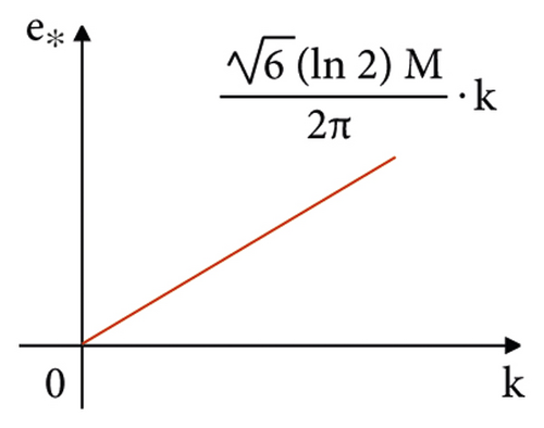
By observing the expression of e^∗, we can know the relationship between the optimal effort level e^∗ and M and the relationship between the optimal effort level e^∗ and k, which are shown in Figure 5.

From the above analysis, it is easy to draw the following conclusions.

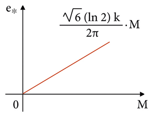
Conclusion 1. As shown in Figure 5(a), e^∗ changes with the change of M, that is, the size of e^∗ and M are proportional. It increases as M increases. It shows that if the M set by the principal in advance is larger, that is to say, the larger the upper limit of the change rate of the emotional output that it can accept in advance, the more it can motivate the agent to make a higher degree of effort. Conversely, too high a level of effort cannot be motivated.

Conclusion 2. As shown in Figure 5(b), e^∗ is proportional to the size of k, which decreases as k decreases. It shows that if the principal knows that the agent's sensitivity to the change of the emotional output is very small, it is reluctant to motivate the effort level that is too high. On the contrary, if the agent is very sensitive to the change of emotional output, the principal is more willing to motivate the agent to pay a higher level of effort, that is, e^∗ is proportional to the rate of change of the agent's utility function about the emotional output.

3. Multilingual Speech Emotion Research Based on Data Mining

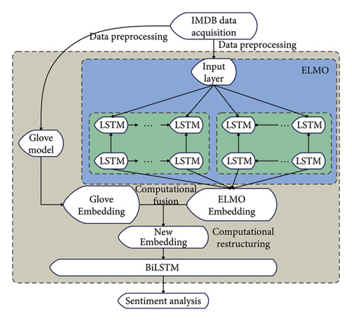
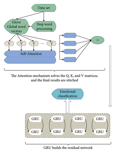
This paper proposes the GE-BiLSTM model. The key part is that the pretrained language model is used to obtain word vectors containing contextual information by training the language model, and combined with the global word vector generated by the traditional Glove, the connection between words is improved. Training word vectors for the purpose of a language model can better capture emotional factors, and a bidirectional LSTM network further extracts text features and improves classification accuracy. The flow chart of the emotion analysis model is shown in Figures 6–8.

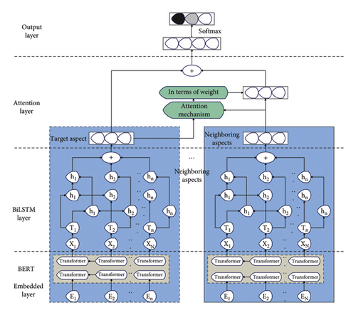
The effect of the multilingual speech emotion research model based on data mining proposed in this paper is verified, and the results of the statistical speech emotion research are shown in Table 1.

1. The effect of multilingual speech sentiment analysis model based on data mining.

Num	Speech sentiment analysis
1	83.28
2	87.49
3	84.98
4	87.14
5	84.67
6	86.67
7	84.29
8	81.27
9	86.92
10	87.97
11	87.04
12	83.18
13	88.47
14	88.64
15	88.57
16	87.80
17	86.27
18	88.60
19	81.69
20	81.72
21	87.67
22	82.44
23	88.97
24	84.86
25	82.24
26	88.25
27	84.00
28	86.05
29	86.57
30	83.98
31	81.37
32	82.58
33	88.90
34	83.17
35	86.54
36	85.94
37	88.71
38	83.58
39	84.51
40	82.94
41	85.17
42	81.58
43	81.98
44	87.27
45	82.09
46	84.58
47	82.71
48	84.27
49	84.16
50	87.80
51	84.38
35	86.54
36	85.94
37	88.71
38	83.58
39	84.51
40	82.94
41	85.17
42	81.58
43	81.98
44	87.27
45	82.09
46	84.58
47	82.71
48	84.27
49	84.16
50	87.80
51	84.38

Through the speech emotion simulation experiment, it can be seen that the multilingual speech emotion analysis model based on data mining proposed in this paper has a good effect on speech emotion analysis.

4. Conclusion

Currently, research on sentiment analysis methods focuses on pretrained language models. The model learns the context-sensitive representation of each word in the input sentence through massive text data, thereby learning generalized grammatical and semantic knowledge and then fine-tuning the network for specific downstream tasks. Pretrained language models have achieved good results in various natural language processing tasks. However, due to the long training time and high computational overhead caused by its large model, it is difficult to deploy it on computers and servers with limited computing power. Therefore, how to compress the model under the premise of ensuring performance and obtain higher accuracy through lightweight models has become a further research direction. In order to improve the effect of speech emotion analysis, this paper combines data mining technology to construct speech emotion research model. Through the speech emotion simulation experiment, it can be seen that the multilingual speech emotion analysis model based on data mining proposed in this paper has a good effect in speech emotion analysis.

Conflicts of Interest

The authors declare no conflicts of interest in relation to this article.

Acknowledgments

This work was supported by Zhejiang University.

Open Research

Data Availability

The labeled dataset used to support the findings of this study is available from the corresponding author upon request.

References

1 Schuller B. W., Speech emotion recognition: two decades in a nutshell, benchmarks, and ongoing trends, Communications of the ACM. (2018) 61, no. 5, 90–99, https://doi.org/10.1145/3129340, 2-s2.0-85046550795.
10.1145/3129340
Web of Science® Google Scholar
2 Vrysas N., Kotsakis R., Liatsou A., Dimoulas C. A., and Kalliris G., Speech emotion recognition for performance interaction, Journal of the Audio Engineering Society. (2018) 66, no. 6, 457–467, https://doi.org/10.17743/jaes.2018.0036, 2-s2.0-85049218623.
10.17743/jaes.2018.0036
Web of Science® Google Scholar
3 Sailunaz K., Dhaliwal M., Rokne J., and Alhajj R., Emotion detection from text and speech: a survey, Social Network Analysis and Mining. (2018) 8, no. 1, 28–26, https://doi.org/10.1007/s13278-018-0505-2, 2-s2.0-85045116585.
10.1007/s13278-018-0505-2
Google Scholar
4 Zhao Z., Bao Z., Zhao Y., Zhang Z., Cummins N., Ren Z., and Schuller B., Exploring deep spectrum representations via attention-based recurrent and convolutional neural networks for speech emotion recognition, IEEE Access. (2019) 7, no. 2, 97515–97525, https://doi.org/10.1109/access.2019.2928625, 2-s2.0-85070274012.
10.1109/ACCESS.2019.2928625
Web of Science® Google Scholar
5 Salido Ortega M. G., Rodríguez L. F., and Gutierrez-Garcia J. O., Towards emotion recognition from contextual information using machine learning, Journal of Ambient Intelligence and Humanized Computing. (2020) 11, no. 8, 3187–3207, https://doi.org/10.1007/s12652-019-01485-x, 2-s2.0-85073982754.
10.1007/s12652-019-01485-x
Web of Science® Google Scholar
6 Koolagudi S. G., Murthy Y. V. S., and Bhaskar S. P., Choice of a classifier, based on properties of a dataset: case study-speech emotion recognition, International Journal of Speech Technology. (2018) 21, no. 1, 167–183, https://doi.org/10.1007/s10772-018-9495-8, 2-s2.0-85044615641.
10.1007/s10772-018-9495-8
Google Scholar
7 Alghifari M. F., Gunawan T. S., and Kartiwi M., Speech emotion recognition using deep feedforward neural network, Indonesian Journal of Electrical Engineering and Computer Science. (2018) 10, no. 2, 554–561, https://doi.org/10.11591/ijeecs.v10.i2.pp554-561, 2-s2.0-85042761850.
10.11591/ijeecs.v10.i2.pp554-561
Google Scholar
8 Gu Y., Wang Y., Liu T., Ji Y., Liu Z., Li P., Wang X., An X., and Ren F., EmoSense: computational intelligence driven emotion sensing via wireless channel data, IEEE Transactions on Emerging Topics in Computational Intelligence. (2020) 4, no. 3, 216–226, https://doi.org/10.1109/tetci.2019.2902438.
10.1109/TETCI.2019.2902438
Google Scholar
9 Alswaidan N. and Menai M. E. B., A survey of state-of-the-art approaches for emotion recognition in text, Knowledge and Information Systems. (2020) 62, no. 8, 2937–2987, https://doi.org/10.1007/s10115-020-01449-0.
10.1007/s10115-020-01449-0
Web of Science® Google Scholar
10 Tan L., Yu K., Lin L., Cheng X., Srivastava G., Lin J. C. W., and Wei W., Speech emotion recognition enhanced traffic efficiency solution for autonomous vehicles in a 5G-enabled space–air–ground integrated intelligent transportation system, IEEE Transactions on Intelligent Transportation Systems. (2022) 23, no. 3, 2830–2842, https://doi.org/10.1109/tits.2021.3119921.
10.1109/TITS.2021.3119921
Web of Science® Google Scholar
11 Alghifari M. F., Gunawan T. S., Qadri S. A. A., Kartiwi M., and Janin Z., On the use of voice activity detection in speech emotion recognition, Bulletin of Electrical Engineering and Informatics. (2019) 8, no. 4, 1324–1332.
Google Scholar
12 Buitelaar P., Wood I. D., Negi S., Arcan M., McCrae J. P., Abele A., Robin C., Andryushechkin V., Ziad H., Sagha H., Schmitt M., Schuller B. W., Sanchez-Rada J. F., Iglesias C. A., Navarro C., Giefer A., Heise N., Masucci V., Danza F. A., Caterino C., Smrz P., Hradis M., Povolny F., Klimes M., Matejka P., and Tummarello G., Mixedemotions: an open-source toolbox for multimodal emotion analysis, IEEE Transactions on Multimedia. (2018) 20, no. 9, 2454–2465, https://doi.org/10.1109/tmm.2018.2798287, 2-s2.0-85040988311.
10.1109/TMM.2018.2798287
Web of Science® Google Scholar
13 Md Saad M., Jamil N., and Hamzah R., Evaluation of support vector machine and decision tree for emotion recognition of Malay folklores, Bulletin of Electrical Engineering and Informatics. (2018) 7, no. 3, 479–486, https://doi.org/10.11591/eei.v7i3.1279, 2-s2.0-85052713014.
10.11591/eei.v7i3.1279
Google Scholar
14 Kumar T. S. and Senthil T., Construction of hybrid deep learning model for predicting children behavior based on their emotional reaction, Journal of Information Technology and Digital World. (2021) 3, no. 1, 29–43, https://doi.org/10.36548/jitdw.2021.1.004.
10.36548/jitdw.2021.1.004
Google Scholar
15 Mendoza-Palechor F., Menezes M. L., Sant’Anna A., Ortiz-Barrios M., Samara A., and Galway L., Affective recognition from EEG signals: an integrated data-mining approach, Journal of Ambient Intelligence and Humanized Computing. (2019) 10, no. 10, 3955–3974, https://doi.org/10.1007/s12652-018-1065-z, 2-s2.0-85054326423.
10.1007/s12652-018-1065-z
Web of Science® Google Scholar
16 Moon J., Ke F., and Sokolikj Z., Automatic assessment of cognitive and emotional states in virtual reality-based flexibility training for four adolescents with autism, British Journal of Educational Technology. (2020) 51, no. 5, 1766–1784, https://doi.org/10.1111/bjet.13005.
10.1111/bjet.13005
Web of Science® Google Scholar
17 Schuller D. M. and Schuller B. W., A review on five recent and near-future developments in computational processing of emotion in the human voice, Emotion Review. (2021) 13, no. 1, 44–50, https://doi.org/10.1177/1754073919898526.
10.1177/1754073919898526
Web of Science® Google Scholar
18 Demircan S. and Kahramanli H., Application of fuzzy C-means clustering algorithm to spectral features for emotion classification from speech, Neural Computing & Applications. (2018) 29, no. 8, 59–66, https://doi.org/10.1007/s00521-016-2712-y, 2-s2.0-84996868118.
10.1007/s00521-016-2712-y
Web of Science® Google Scholar
19 Ford E., Oswald M., Hassan L., Bozentko K., Nenadic G., and Cassell J., Should free-text data in electronic medical records be shared for research? A citizens' jury study in the UK, Journal of Medical Ethics. (2020) 46, no. 6, 367–377, https://doi.org/10.1007/s00521-016-2712-y, 2-s2.0-84996868118.
10.1136/medethics-2019-105472
PubMed Web of Science® Google Scholar

All articles

Multilingual Speech Emotion Research Based on Data Mining

Abstract

1. Introduction

2. Speech Emotion Recognition Algorithm

2.1. Expected Value of Fuzzy Variable Function