Computational Intelligence and Neuroscience

Volume 2022, Issue 1 4822212

Research Article

Open Access

Bayesian Estimation of Different Scale Parameters Using a LINEX Loss Function

M. A. Mohammed,

M. A. Mohammed

orcid.org/0000-0001-6435-0323

Department of Mathematics, Al-Lith University College, Umm Al-Qura University, Mecca, Saudi Arabia uqu.edu.sa

Department of Mathematics, Faculty of Science, Assiut University, Assiut, Egypt aun.edu.eg

Search for more papers by this author

Sundus N. Al-Aziz,

Sundus N. Al-Aziz

orcid.org/0000-0002-0860-6555

Department of Mathematical Sciences, College of Science, Princess Nourah bint Abdulrahman University, P.O. Box 84428, Riyadh 11671, Saudi Arabia pnu.edu.sa

Search for more papers by this author

Eateraf M. A. Al Sumati,

Corresponding Author

Eateraf M. A. Al Sumati

[email protected]

orcid.org/0000-0001-7925-3331

Department of Statistics & Informatics, Faculty of Administrative Sciences, University of Aden, Aden, Yemen

Search for more papers by this author

Emad E. Mahmoud,

Emad E. Mahmoud

orcid.org/0000-0003-2757-2765

Department of Mathematics and Statistics, College of Science, Taif University, P.O. Box 11099, Taif 21944, Saudi Arabia tu.edu.sa

Search for more papers by this author

M. A. Mohammed,

M. A. Mohammed

orcid.org/0000-0001-6435-0323

Department of Mathematics, Al-Lith University College, Umm Al-Qura University, Mecca, Saudi Arabia uqu.edu.sa

Department of Mathematics, Faculty of Science, Assiut University, Assiut, Egypt aun.edu.eg

Search for more papers by this author

Sundus N. Al-Aziz,

Sundus N. Al-Aziz

orcid.org/0000-0002-0860-6555

Department of Mathematical Sciences, College of Science, Princess Nourah bint Abdulrahman University, P.O. Box 84428, Riyadh 11671, Saudi Arabia pnu.edu.sa

Search for more papers by this author

Eateraf M. A. Al Sumati,

Corresponding Author

Eateraf M. A. Al Sumati

[email protected]

orcid.org/0000-0001-7925-3331

Department of Statistics & Informatics, Faculty of Administrative Sciences, University of Aden, Aden, Yemen

Search for more papers by this author

Emad E. Mahmoud,

Emad E. Mahmoud

orcid.org/0000-0003-2757-2765

Department of Mathematics and Statistics, College of Science, Taif University, P.O. Box 11099, Taif 21944, Saudi Arabia tu.edu.sa

Search for more papers by this author

First published: 30 April 2022

https://doi.org/10.1155/2022/4822212

Citations: 2

Academic Editor: Ahmed Mostafa Khalil

Share a link

Email
Wechat
Bluesky

Abstract

The LINEX loss function, which climbs exponentially with one-half of zero and virtually linearly on either side of zero, is employed to analyze parameter analysis and prediction problems. It can be used to solve both underestimation and overestimation issues. This paper explained the Bayesian estimation of mean, Gamma distribution, and Poisson process. First, an improved estimator for μ² is provided (which employs a variation coefficient). Under the LINEX loss function, a better estimator for the square root of the median is also derived, and an enhanced estimation for the average mean in such a negatively exponential function. Second, giving a gamma distribution as a prior and a likelihood function as posterior yields a gamma distribution. The LINEX method can be used to estimate an estimator using posterior distribution. After obtaining , the hazard function and the function of survival estimators are used. Third, the challenge of sequentially predicting the intensity variable of a uniform Poisson process with a linear exponentially (LINEX) loss function and a constant cost of production time is investigated using a Bayesian model. The APO rule is offered as an approximation pointwise optimal rule. LINEX is the loss function used. A variety of prior distributions have already been studied, and Bayesian estimation methods have been evaluated against squared error loss function estimation methods. Finally, compare the results of Maximum Likelihood Estimation (MLE) and LINEX estimation to determine which technique is appropriate for such information by identifying the lowest Mean Square Error (MSE). The displaced estimation method under the LINEX loss function was also examined in this research, and an improved estimation was proposed.

1. Introduction

The LINEX loss function is a nonlinear function that climbs exponentially with one end of 0 and virtually exponentially on another [1]. For values approaching zero, this error function reduces to squared error loss. For calculating the binomial variable, the LINEX loss function is used. This loss function was used to estimate the median of a normally distributed [2]. Consider the prediction error in the perspective of exponential distribution reliability analysis. Then, using the LINEX loss function, Bayesian mean and square mean estimations of a normally distributed were investigated. Under the LINEX loss function, the MMSE criterion is unacceptable. The uniformly minimum risk unbiased (UMRU) estimator under the LINEX loss function can be found using information and facts if there is underestimation and overestimation in real-life situations [3]. The exponential distribution is a well-known distribution that may be used in a variety of fields, including science, economy, and demographics [4]. It is a well-known one-parameter distribution that is frequently utilized in model studies [5].

A linear exponential loss function (LINEX) is developed to estimate the scale parameter and reliability function of the inverse Weibull distribution (IWD) based on lower record values [6]. The Bayesian technique is also necessary for this study, in addition to employing Maximum Likelihood to estimate the parameters. It creates a posterior probability by combining an exponential distribution’s likelihood value with a prior [7]. Because altering the value to 1 and having an Exponential distribution, the Gamma distribution is an appropriate prior for it. In statistics, there are a few estimating approaches. One of them is Bayesian, which finds the posterior distribution using the likelihood function and prior distribution [8]. The data is exponentially distributed, and the posterior distribution will be constructed using a Gamma distribution as its prior. Let F be sometimes referred to as the failure time random variable because it is defined as the time of failure of the object known to exist at time t = 0. If F is the time to failure, the likelihood of still operating at time t is like the probability that the failure will occur later (mathematical model higher) than t. The following equation is the definition of the survival density function (SDF), probability density function (PDF), and hazard rate function (HRF).

(1)

The task of establishing appropriate halting rules is frequently and analytically intractable. Because determining explicit optimum ending times is challenging, numerous approaches were proposed to obtain “asymptotically” optimal regulations [9]. For example, it offered simple but appealing large enough sample approximations to optimal timings, dubbed asymptotically pointwise optimal (APO) rules, and demonstrated that APO rules were asymptotically optimal (AO) under a second scenario. Many publications have examined the APO rule and how it might be used to address those other challenges [10]. Discrete-time events are the focus of the studies in these publications. They discussed how the LINEX error function operated, but still, no specifics or practical solutions were provided on how the LINEX loss function changes the shape variable and error value [11]. Considering the LINEX loss method’s versatility in estimating a location parameter, it does not seem to be useful for estimating scale variables and other values. For two variables, Bayes and probability estimators are used [12]. Under hazard and survival variables used in experiments and analysis methods, Weibull using unfiltered observations is examined.

In continuous-time processes, the idea of the asymptotic element-wise optimization problem is expanded from discrete-time processes [11]. Additionally, with a squared error loss, the APO procedures for predicting the intensities of a homogeneity Poisson process are AO for random priors and asymptotically nondeficient for conjugation priors [13]. Later, it generalized a conclusion for continuous-time processes and demonstrated that under a linear exponential (LINEX) loss function, the APO rules for such a Poisson distribution are AO for such corresponding priors [14]. The LINEX loss function was officially created, and its properties were investigated further. It is a handy asymmetrical nonlinear function that increases dramatically on one end of zero and gradually on the other [15]. Much research has looked into estimating issues with LINEX loss function [16]. After analyzing the data, it assigns relative weights to each given value. Approximations to Bayesian inference exist, such as the Specific Noninformative Prior [17]. Linear Exponential Loss Function, Lindley Approximation, General Entropy Loss Function, and Squared Error Loss Function are all examples of linear, exponential loss functions.

2. Related Work

The Weibull distribution is commonly used in lifespan data modeling and analysis [14]. The considered wide range of a two-parameter Weibull distribution having given shape is estimated in this study. How to use estimated parameters is discussed. Under the LINEX loss function, the Bayes estimator is produced utilizing Jeffreys’ prior. Using generated data sets, the overall performance of the estimation techniques is calculated in small and large sampling for overestimation and underestimation. It has been discovered that the Bayes estimator performed best in observational studies and then when overstatement is much more important than underestimating.

In technology, science, and other fields, the Weibull distribution has been identified as among the most effective distributions for predicting and evaluating lifetime data [18]. To find the most effective approach for calculating its characteristics, the Bayesian estimate strategy for estimation methods, which competes with other estimation approaches, has suddenly received a lot of attention. For assessing the 2 different Weibull failure time distributions, the achievement of the maximum likelihood method and Bayes estimator using expansions of Jeffreys prior knowledge with three wavelet coefficients, namely, the sequential exponential loss, general electron density loss, and square error linear function. Through a simulation analysis with varied sample sizes, these approaches are evaluated using mean square error. The findings demonstrate that for certain values of extensions of Jeffreys’ prior, the Bayesian estimator utilizing extensions of Jeffreys’ prior with linear exponentially error function has the minimum mean square error and actual bias both for weighting factor and the significant impact.

Dey introduced Bayes’ estimation technique for such an Inverse Rayleigh distribution’s unknown quantity (IRD) [19]. Utilizing noninformative prior, Bayes estimation techniques are derived for symmetrical (squared error (SE) loss) and asymmetrical linear exponential loss functions. The estimators’ system is assessed based on its relative hazard under two wavelet coefficients. They also construct the reliability method’s Bayesian estimation method using symmetrical and asymmetrical loss functions and compare their efficiency that used a Monte Carlo simulation analysis. Lastly, to highlight the findings, a numerical investigation is offered.

Gupta presented a new method for predicting the variable of the Rayleigh distribution, Bayesian and E–Bayesian estimate methods are provided in this study [20]. The parameter’s Bayes estimation is calculated using the LINEX loss function and the concept that the prior probability is relevant, i.e., gamma distribution. Furthermore, a simulation study utilizing MATLAB software was used to compare the E-Bayes estimation method with related Bayes estimators.

The work of Lee and Hwang looks at the challenge of progressively predicting the average of a Poisson process in a Bayesian network using a LINEX (linear exponential) loss function and a fixed price per experience [21]. For arbitrary priors, an approximation pointwise optimum rule with such a distribution function is developed and proven to be exponential optimal. An actual data set is used to demonstrate the suggested monotonically elementwise optimum rule.

3. Proposed Methodology

Let us consider a₁, a₂, ……a_n an n-person representative sample from such an average distribution with median μ and variance σ². Assume that compared to the population median with minimum error , the sample mean (σ²/n) is an adequate and accurate estimator. The standard approach of comparing estimation methods for the significant feature using mean square error (MSE) may not provide a clear favorite for scale parameters [22]. Limiting the class of estimators is one technique to make the task of finding the “best estimator” more tractable. Consider impartial and partially invariant estimation techniques as a popular approach to limiting the category of estimation techniques.

The improvement of the estimator

is in the estimator class

and it shows the MSE represented in the equation:

(2)

U(a) = θ, R(a) = θ² and v = 1 in the negative exponential distribution (NED). The scale parameter is θ, and the improved estimator is with an MSE E₁ = (θ²/n + 1) lower than (θ²/n). In a normal distribution with mean μ and variance σ², where σ² acts as a standard deviation and the maximum likelihood estimate are (MLE), the estimators for σ² (the unbiased estimator).

Thus, MSE (M²) = (2σ⁴/n) and then MSE. (M²) = (2σ⁴/n − 1)

The LINEX loss equation is given below:

(3)

where x and y are the shapes and a scale parameter.

If |x|⟶0, Square inaccuracy is the result of the LINEX loss.

Mean Estimation using a LINEX loss function.

x ≠ 0, and if the bc = x, Later, this procedure would equal y(e^xΔ − zΔ − 1)

The loss function of LINEX minimizes the squared error if |x|⟶0.

For calculating, the constant form of LINEX loss was used. LINEX loss in its symmetric form is given in the equation:

(4)

where

Consider the estimator Y = xc 1 in the case of a normally distributed with variance and mean both equal to two. LINEX loss in its invariant form is given in the following equation:

(5)

In a negative exponential distribution,

(6)

From equation (8), then the value of minimum z could be shown in the following equation:

(7)

The proposed estimation is with a. MinQ(x, Δ^∗) = x − (n + 1)(x − e^(−x/n+1))

As a result, under the LINEX loss function, the minimum mean squared error is unacceptable [7]. This can get the minimum if the differentiate equation (5) is about c and equal to zero:

(8)

The values of z can be calculated given the values of n, v ≥ 1 and 0 ≤ x ≤ 0.6. Then, get the lowest risk by plugging the c_min into equation (5) [23]. Figures 1–3 show the relative effectiveness of the estimator E₁ in comparison to E^′ for v = 2.00(2.25)2.50, x = 0.2(0.4)0.6 and n = 5(5)20. The figure illustrates that if v ≥ 1 is greater than 1, the estimator outperforms with smaller n values and a level up to 2.00.

Details are in the caption following the image — **Figure 1**
Open in figure viewer PowerPoint

Estimator relative efficiency E₁E^′ for v = 2.00.

Also, under the LINEX loss function, the Bayesian estimator for median and square of group means of normally distributed was investigated. In the case of a negative exponential function, the answer for the scale parameter by using an invariant form of the LINEX error function is

(9)

(Gamma (1, n)) adopts a chi-square distribution with 2n degrees of freedom. It established a modified Bessel formula as follows:

(10)

The estimator MVRU for θ is as follows:

(11)

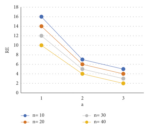
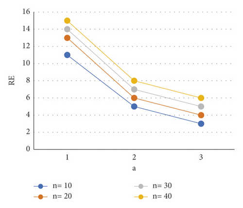
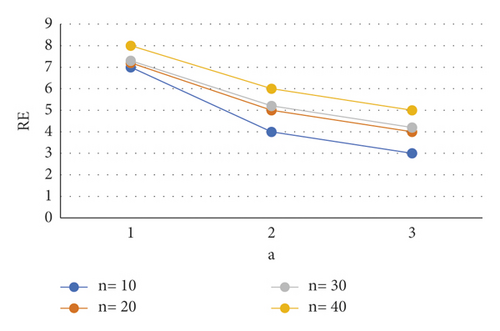
This demonstrates that in the LINEX loss function, adequate statistics x can also be used to determine the UMRU estimation.

3.1. Maximum Likelihood Estimation

Censoring is a method of dealing with incomplete data that occurs as a result of events such as death, loss, or removal from observation. Variables V₁, …V_n denote n individual lifespan, as per [24]. A lifetime or a counting time is denoted by the letter v_i. The censoring or state indication for t₁ is the variable δ_i = 1 if V_i = t_i and 0 if V_i > t_i. The value t1 is calculated using min(V_i, Z_i), i = 1,2,3, …, n, where V_i is the length of their remission assessed from the beginning of the course and Z_i is the period between the beginning of the study and the end of the study. It is possible to construct the likelihood function of censored data for observations (t_i, δ_i)i = 1,2, …, n.

(12)

The exponential distribution likelihood function for the observation (t_i, δ_i)i = 1,2,3, …, n is calculated as follows:

(13)

Then, as shown above, discover a natural logarithm of the likelihood function.

(14)

By deriving k to the parameter λ, , obtain the following:

(15)

A Maximum Likelihood Estimated is obtained. Subsequently, both the equation of survival and the rate of hazard are composed.

(16)

and are based on Maximum Probability [2]. The ratio of hazard and survival model is estimated.

3.2. The Poisson Process Rules of APO and AO

Let {N(f) : f ≥ 0} be a Poisson process that is homogeneous but has an undetermined amplitude parameter. It is desired to predict θ by

, a specific topic to the LINEX loss and the sampling cost after observing the process during the time interval [0, f].

(17)

where

is the price per unit time, c is the LINEX loss. As can be seen, c can also be thought of as a proportional weight to the LINEX loss. Across all stopping periods and estimation methods, the goal is to minimize the Bayes hazard. Concerning the defect

, the LINEX loss is a positive and asymmetrical function [25]. It is beneficial in estimating difficulties when underestimation or overestimation is deemed more dangerous than the other. The shape of the object is determined by the variable a. When the x > 0, it means that overestimation is more expensive than underestimation. When x < 0 is present, the inverse is true.

Assume, which has a θ constant density Ψ concerning the Lebesgue measurement, with L(θ) < ∞ and L(e^−xθ) < ∞, respectively. For ℱ_' = σ(N(u) : 0 ≤ u ≤ f) for f ≥ 0 and ℱ_∞ be the smallest -field comprising all of ℱ_' events for all f ≥ 0. The Bayesian estimation is very well recognized as the best estimation with a stop time of P.

(18)

where ℱ_p = {X ∈ ℱ_∞|X|∩{N ≤ f} ∈ ℱ_f forall f ≥ 0}. The Bayes hazard of a Bayesian sequential approach

is therefore equal to the following:

(19)

This suggests an APO condition in a Poisson distribution as in Section 3.2.

In Theorem 1, the halting rule

and the Bayesian sequential process

are proven to be APO and AO, respectively. To establish Theorem 1, first establish some representations, followed by the development of some supplementary results. Let

be the maximum likelihood estimation θ of based on {W(i) : 0 ≤ i ≤ f}, and define Ψ^∗(a|ℱ_f) as the posterior probability of

given ℱ_f for simplicity. Thus,

(20)

Define the random numbers

(21)

For

and B_f(a) = 0 otherwise, then

(22)

For and Q_t(b) = −1.

3.3. The LINEX Loss Function of Bayesian

In statistical methods studies, the Bayesian Process is the well-estimating method [26]. The Bayesian estimate has three different loss functions. In Bayesian estimation, another of the loss functions is LINEX. As per Zellner, the LINEX loss method’s posterior prediction [27]. One of the Bayesian techniques is the LINEX loss function. The variable estimation of λ is represented by

that under LINEX error function is constructed while using Zellner’s method.

(23)

To expose the posterior equation which can be utilized to find a parameter estimate BL under the Bayesian LINEX loss function.

(24)

As a result of (24) get the appropriate estimation method under the LINEX loss function:

(25)

Furthermore, equation (26) describes the survival and hazard functions [16] that under a LINEX loss function,

(26)

3.4. Square Estimation of Mean by Using LINEX Loss Function

In the normal distribution, thus known as follows:

(27)

That implies the following:

(28)

Let us consider the minimum value of t₂

(29)

Then the estimator proposed is represented as follows:

(30)

If v is known (30); if v is unknown; then MVUE for μ² is as follows:

(31)

N could be negative for smaller values of n, hence proposed a biassed estimator for μ² as

and looked at its huge sample features [28]. To generate an estimator with a certain mean square error as S but a reduced bias than S for huge sample sizes n,

(32)

For the estimator, the invariant expression of the LINEX loss function

(33)

This gets to t₄ and equal to zero by simplifying this solution.

(34)

Mostly in the case of a negative exponential function [29], the enhanced estimator is used.

In the case of N.E.D. with E (θ, θ), and

(35)

The Function of LINEX loss on the invariant form is as follows:

(36)

This has the following:

(37)

When this formula is differentiated about z₅ and equated to zero, obtain the following:

(38)

When again differentiating equation (37) about z₅,

(39)

And z₅ lies among

(40)

Equating to zero and differentiating solution (37) concerning z₅

(41)

3.5. Nondeficiency of Asymptotic

In this part, develop a better understanding of when the strength parameter’s previous distributions have the following density of gamma:

(42)

where α > 0 and β > 0 are both true. There is a formulation of the posterior density of a particular ℱ_t of the type Ψ(θ; α + R(t), β/(tβ + 1)) for t ≥ 0 fixed. It is simple to prove that the posterior densities of a given FS have a version of Ψ(θ; α + R(d), β/(dβ + 1)) for an unspecified stopping time D [30]. The homogeneous Poisson process of intensity even during the period [0, t] then the Bayesian estimator is provided by Assuming αβ + 1 > 0, if analyze the homogeneous Poisson process in intensity θ even during the time-period [0, t] then the Bayesian estimator of θ is provided by the following:

(43)

and the risk it represents in the future is from the sort

(44)

Let

(45)

where

(46)

As a result of Taylor’s theorem,

(47)

Thus,

(48)

In the gamma prior example, the form of

provided can be reorganized as follows:

(49)

For any c > 0, and , it can be seen that c > 0. Theorem 1 states that in the gamma previous also with requirements α > 0, β > 0, and αβ + 1 > 0, the halting rule and the Bayesian sequential method are APO and AO, accordingly (Mahmoudi 2012). In addition, Theorem 2 in this statement demonstrates that the Bayes sequential process is asymptotically quasi in this instance.

Let

(50)

(51)

Establish several auxiliary results before and use them to establish the major theorem.

4. Numerical Study and Discussion

4.1. Estimation Error LINEX Loss Function

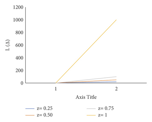
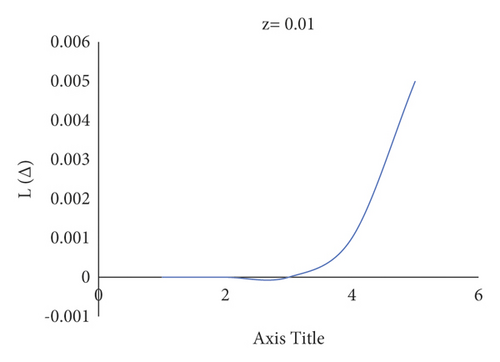
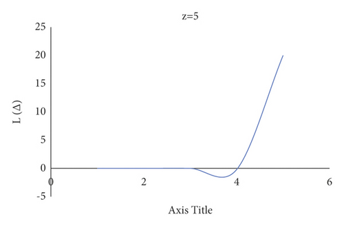
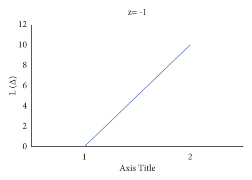
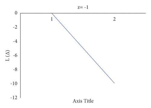
Consider the estimation error as . Figure 4 shows how a negative value of c gives more importance to underestimation, whose quantity describes the level of asymmetry. Figure 5 shows that a positive value of c will not provide an additional load to overestimation, whose quantity represents the extent of asymmetry. The LINEX loss function is essentially symmetric for small values of |z| but not that far from the mean square error loss function in Figure 6. The LINEX loss function is essentially asymmetric for large values of |z| in Figure 7. When the prediction error is in Figure 8, it climbs almost continuously z > 0, and when the prediction error is in Figure 9, it rises practically exponentially.

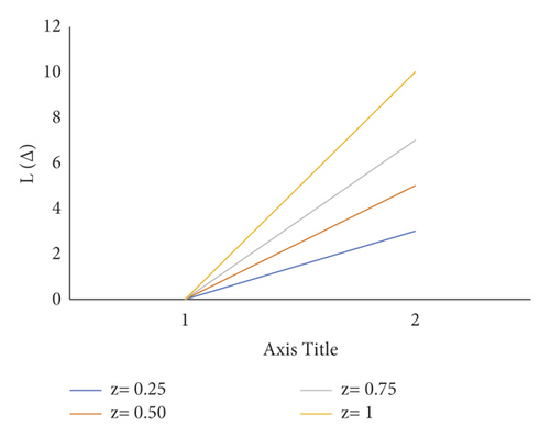
This offers the APO rules and the Bayesian estimate under gamma prior supplied and evaluates the APO rule’s Bayesian hazard to the second element of the Bayesian risk of an optimum halting rule (or APO rule). Let be the estimation for such Bayes risk of the APO rule , and ; that is, the second level of the Bayesian hazard of the optimum halting rule, depending on Theorem 1.

The estimates of the APO principle , the Bayesian estimator , the calculated Bayes risk , the second-order , and the adjusted mean inaccuracy of Bayes risk for various values of x, α, β, and z. Because the requirements are different for a < 0, the variables of () are selected as (1.5, 0.2), (2.5, 0.1), and (2.5, 0.1). of Theorem 1 can be expressed as α > 1 and 0 < β < −1/a. Table 1 shows that when z drops, the estimates increase and and almost decrease. Furthermore, when z gets smaller, the estimations of absolute errors of Bayesian hazard Δ_z approach to zero.

Table 1. The data for gamma (α, β) with a variety of (α, β) and z values.

z					Δ_z					Δ_z
	(α,β) = (2.5, 0.4)					(α,β) = (3.5, 0.2)
10	0.4324	0.2347	0.7632	0.7352	−0.4567	0.0876	0.5293	0.2734	−3.8752	−1.3747
0.01	1.2346	0.2765	0.2763	0.3678	−0.3456	0.7653	0.2636	0.2863	−0.1254	−2.3752
0.05	1.2487	0.3248	0.6427	0.9782	−0.3657	1.4321	0.3826	0.2737	0.0274	2.7358
0.001	2.4567	0.2654	0.2753	0.7643	0.1236	8.6537	0.3362	0.3823	0.2735	0.2837
0.005	10.9876	0.3875	0.3875	0.8752	0.1432	11.7526	0.2763	0.2836	0.2934	0.2863
0.0001	13.9769	0.2873	0.2643	0.9826	0.0123	23.9875	0.3826	0.2733	0.2647	0.3754
0.0005	23.8765	0.3864	0.3625	0.2764	−0.0154	35.7521	0.2863	0.3826	0.2735	0.2647

The survival likelihood of patients after therapy using the MLE and Bayesian LINEX Loss functions: Both findings show that the estimated value is bigger than that of the real value, but the Bayesian LINEX estimated value is closer to a survival value than that of the MLEs. The outcome reveals that all variables are inversely proportional to time. Patients’ chances of survival are decreasing and converging to zero in less than three years. It signifies that the treatment’s effects will fade with time. In around 10 days of varying ranges, the decreasing level of survival chance is around 10%. The survival report’s hazard function is linked to the degeneration rate. Table 2 shows the hazard values estimation using both the MLE and Bayesian LINEX Loss functions.

Table 2. MLE hazard values and estimation of the Bayes LINEX loss function.

Hazard	Hazard value estimation using MLE	Hazard value estimation using Bayesian LINEX
0.008231808	0.0075643263	0.0076543276

The hazard value is used to calculate the dependability rate of failure. The rate of failure of the true value utilizing MLE and Bayesian LINEX is 0.8231808%, 0.7564323%, and 0.76543276%, respectively, according to Table 2. It means that the Bayesian estimate is closer to the real number than that of the MLE estimate. By looking at the lowest MSE of both outcomes, one technique to discover the optimal method would be to calculate Mean Squared Error (MSE). Table 3 depicts them.

Table 3. Survival and hazard MSE values for MLE and Bayes LINEX loss functions.

Mean square error	Survival	Hazard
Bayesian LINEX loss function	2.7872E − 08	0.000303142
MLE	2.91727E − 06	0.000245904

The Value of MSE of Hazard and survival with Bayes LINEX Loss Function would be less than MSE values of hazard and survival over MLE, as shown in Figures 10 and 11.

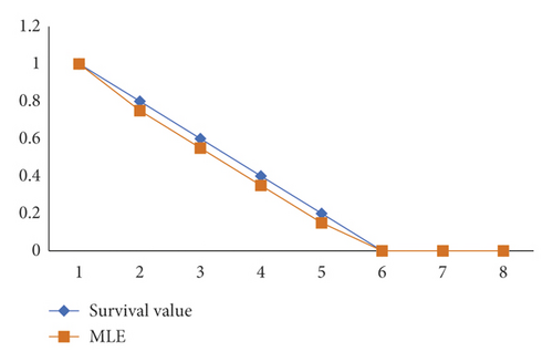
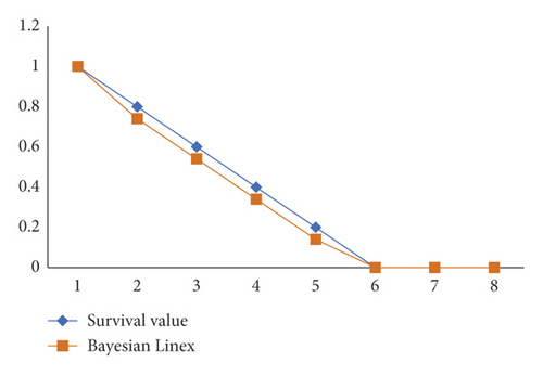
Although both graphs 1 and 2 indicate a varying value well with the actual cost of survival chances, graph 2’s curve does have a faster distance between an actual and Bayesian value.

5. Conclusion

The LINEX loss function, when using comparative estimation error, gives preference to overestimation in displaying that the allocation is irregular for negative numbers of the scaling factor, while it also gives weight to overestimation in displaying that the transfer is asymmetric for positive values. It lends more importance towards overestimation, which indicates the degree of imbalance, for positive attributes of c. The criterion of the LINEX loss function is achieved for positive attributes of the scaling factor. However, this is more widely disseminated than the initial random sample. In this example, it is also clear that prediction error, rather than estimation of comparative error, performs better when the LINEX loss function is used. As a result, if the LINEX loss function performs better, the estimated error should be utilized rather than the estimation of relative error. Second, the rate of hazard and period of article observation plays an important influence in determining survival value. These are approximately equal to the chances of survival. Finally, the MSE demonstrates that the Bayes LINEX Loss function outperforms the MLE. For future studies, the derivation of the posterior distribution for the distribution estimation under squared error could be explained using informative and noninformative priors.

Conflicts of Interest

The authors declare that there are no conflicts of interest regarding the publication of this paper.

Acknowledgments

This paper was supported by the Taif University Researchers Supporting Project number (TURSP-2020/20), Taif University, Taif, Saudi Arabia.

Open Research

Data Availability

Data are available from the corresponding author upon request.

References

1 Singh B. K., Estimation of mean and its function using asymmetric loss function, International Journal of Soft Computing, Mathematics and Control (IJSCMC). (2013) 2, 27–44.
Google Scholar
2 Abbas K., Abbasi N. Y., Ali A., Khan S. A., Manzoor S., Khalil A., Khalil U., Khan D. M., Hussain Z., and Altaf M., Bayesian analysis of three-parameter frechet distribution with medical applications, Computational and Mathematical Methods in Medicine. (2019) 2019, 8, 9089856, https://doi.org/10.1155/2019/9089856, 2-s2.0-85063447065.
10.1155/2019/9089856
PubMed Web of Science® Google Scholar
3 Panahi H. and Asadi S., Analysis of the type-II hybrid censored burr type XII distribution under LINEX loss function, Applied Mathematical Sciences. (2011) 5, 3929–3942.
Google Scholar
4 Rizki S. W., Mara M. N., and Sulistianingsih E., Survival bayesian estimation of exponential-gamma under LINEX loss function, Journal of Physics: Conference Series. (2017) 855, 012036, https://doi.org/10.1088/1742-6596/855/1/012036, 2-s2.0-85023646960.
10.1088/1742-6596/855/1/012036
Google Scholar
5 Afifi W. A. and El-Bagoury A. H., Optimal multiplicative generalized linear search plan for a discrete randomly located target, Information Sciences Letters. (2021) 10, no. No. 1, 153–158.
10.18576/isl/100117
Google Scholar
6 Al-Duais F. S., Bayesian estimations under the weighted LINEX loss function based on upper record values, Complexity. (2021) 2021, 7, 9982916, https://doi.org/10.1155/2021/9982916.
10.1155/2021/9982916
Web of Science® Google Scholar
7 Al-Duais F. and Alhagyan M., Bayesian estimates based on record values under weighted LINEX loss function, Pakistan Journal of Statistics and Operation Research. (2020) 16, 11–19, https://doi.org/10.18187/pjsor.v16i1.2854.
10.18187/pjsor.v16i1.2854
Web of Science® Google Scholar
8 Wei S., Wang C., and Li Z., Bayes estimation of lomax distribution parameter in the composite LINEX loss of symmetry, Journal of Interdisciplinary Mathematics. (2017) 20, no. 5, 1277–1287, https://doi.org/10.1080/09720502.2017.1311043, 2-s2.0-85030855380.
10.1080/09720502.2017.1311043
Google Scholar
9 Hwang L.-C. and Lee C.-H., Bayes sequential estimation for a Poisson process under a LINEX loss function, Statistics. (2013) 47, no. 4, 672–687, https://doi.org/10.1080/02331888.2011.648640, 2-s2.0-84884474446.
10.1080/02331888.2011.648640
Web of Science® Google Scholar
10 Al-Duais F. S., Bayesian analysis of record statistic from the Inverse Weibull distribution under balanced loss function, Mathematical Problems in Engineering. (2021) 2021, 9, 6648462, https://doi.org/10.1155/2021/6648462.
10.1155/2021/6648462
Web of Science® Google Scholar
11 Khatun N. and Matin M. A., A study on LINEX loss function with different estimating methods, Open Journal of Statistics. (2020) 10, no. 01, 52–63, https://doi.org/10.4236/ojs.2020.101004.
10.4236/ojs.2020.101004
Google Scholar
12 Abu-Moussa M. H., Abd-Elfattah A. M., and Hafez E. H., Estimation of stress-strength parameter for Rayleigh distribution based on progressive type-II censoring, Information Sciences Letters. (2021) 10, 101–110.
10.18576/isl/100112
Google Scholar
13 Sana S. and Faizan M., Bayesian estimation using lindley’s approximation and prediction of generalized exponential distribution based on lower record values, Journal of Statistics Applications & Probability. (2021) 10, no. No. 1, 61–75.
10.18576/jsap/100107
Google Scholar
14 Pandey B. N., Dwivedi N., and Pulastya Bandyopadhyay N. D., Comparison between bayesian and maximum likelihood estimation OF scale parameter IN weibull distribution with KNOWN shape under LINEX loss function, Journal of Scientific Research. (2011) 55, 163–172.
Google Scholar
15 Al-Duais F. S., Bayesian analysis of record statistics from the inverse Weibull distribution under balanced loss function, Mathematical Problems in Engineering. (2021) 2021, 9, 6648462.
10.1155/2021/6648462
Web of Science® Google Scholar
16 Arashi M. and Tabatabaey S. M. M., Estimation of the location parameter under LINEX loss function: multivariate case, Metrika. (2010) 72, no. 1, 51–57, https://doi.org/10.1007/s00184-009-0240-9, 2-s2.0-77952543156.
10.1007/s00184-009-0240-9
Web of Science® Google Scholar
17 Ganaie R. A., Rajagopalan V., and Aldulaimi S., The weighted power shanker distribution with characterizations and applications of real life time data, Journal of Statistics Applications & Probability. (2021) 10, no. No. 1, 245–265.
10.18576/jsap/100122
Google Scholar
18 Guure C. B., Ibrahim N. A., and Ahmed A. O. M., Bayesian estimation of two-parameter Weibull distribution using extension of Jeffreys’ prior information with three loss functions, Mathematical Problems in Engineering. (2012) 2012, 1–13, https://doi.org/10.1155/2012/589640, 2-s2.0-84866153551.
10.1155/2012/589640
Web of Science® Google Scholar
19 Dey S., Bayesian estimation of the parameter and reliability function of an inverse Rayleigh distribution, Malaysian Journal of Mathematical Sciences. (2012) 6, no. 1, 113–124.
Google Scholar
20 Gupta I., Bayesian and E- bayesian method of estimation of parameter of Rayleigh distribution- A bayesian approach under LINEX loss function, International Journal of Statistics and Systems. (2017) 12, 791–796.
Google Scholar
21 Lee C.-H. and Hwang L.-C., Asymptotic optimal estimation of Poisson mean under LINEX loss function, Communications in Statistics - Theory and Methods. (2011) 40, no. 23, 4308–4321, https://doi.org/10.1080/03610926.2010.510252, 2-s2.0-84863062048.
10.1080/03610926.2010.510252
Web of Science® Google Scholar
22 Hwang S., Knight J., and Satchell S. E., Forecasting nonlinear functions of returns using LINEX loss functions, Annals of Economics and Finance. (2001) 2, no. 1, 187–213.
Google Scholar
23 Han M., E-bayesian estimation of the exponentiated distribution family parameter under LINEX loss function, Communications in Statistics - Theory and Methods. (2019) 48, no. 3, 648–659, https://doi.org/10.1080/03610926.2017.1417432, 2-s2.0-85043378152.
10.1080/03610926.2017.1417432
Web of Science® Google Scholar
24 Krishna H. and Goel N., Maximum likelihood and Bayes estimation in randomly censored geometric distribution, Journal of Probability and Statistics. (2017) 2017, 12, 4860167, https://doi.org/10.1155/2017/4860167, 2-s2.0-85029379147.
10.1155/2017/4860167
Google Scholar
25 Hwang L.-C., Second order optimal approximation in a particular exponential family under asymmetric LINEX loss, Statistics & Probability Letters. (2018) 137, 283–291, https://doi.org/10.1016/j.spl.2018.01.032, 2-s2.0-85042657679.
10.1016/j.spl.2018.01.032
Web of Science® Google Scholar
26 Al-Duais F. S. and Yousif M., Bayesian and non-Bayesian estimation of the Lomax model based on upper record values under weighted LINEX loss function, Periodicals of Engineering and Natural Sciences. (2020) 8, 1786–1794.
Google Scholar
27 Yousefzadeh F., E-bayesian and hierarchical bayesian estimations for the system reliability parameter based on asymmetric loss function, Communications in Statistics - Theory and Methods. (2017) 46, no. 1, 1–8, https://doi.org/10.1080/03610926.2014.968736, 2-s2.0-84989234952.
10.1080/03610926.2014.968736
Web of Science® Google Scholar
28 Li L., Bayes estimation of parameter of laplace distribution under a new LINEX-based loss function, International Journal of Data Science and Analysis. (2017) 3, no. 6, 85–89, https://doi.org/10.11648/j.ijdsa.20170306.14.
10.11648/j.ijdsa.20170306.14
Google Scholar
29 Guure C. B. and Ibrahim N. A., Approximate Bayesian estimates of Weibull parameters with Lindley's method, Sains Malaysiana. (2014) 43, 1433–1437.
Web of Science® Google Scholar
30 Hwang L.-C., Asymptotic non-deficiency of some procedures for a particular exponential family under relative LINEX loss, Sequential Analysis. (2014) 33, no. 3, 345–359, https://doi.org/10.1080/07474946.2014.916928, 2-s2.0-84902970113.
10.1080/07474946.2014.916928
Web of Science® Google Scholar

Citing Literature

All articles

Bayesian Estimation of Different Scale Parameters Using a LINEX Loss Function

Abstract

1. Introduction

2. Related Work

3. Proposed Methodology

3.1. Maximum Likelihood Estimation

3.2. The Poisson Process Rules of APO and AO

3.3. The LINEX Loss Function of Bayesian

3.4. Square Estimation of Mean by Using LINEX Loss Function

3.5. Nondeficiency of Asymptotic

4. Numerical Study and Discussion

4.1. Estimation Error LINEX Loss Function

5. Conclusion

Conflicts of Interest

Acknowledgments

Open Research

Data Availability

References

Citing Literature

Figures

References

Information

About Wiley Online Library

Help & Support

Opportunities

Connect with Wiley