This article discusses an iterative transformation method via fuzziness that mixtures the Laplace transform with the iterative iterative method. Using Caputo derivative operator, the proposed technique demonstrates the inherent reliability of fractional fuzzy biological population equations with initial fuzzy conditions. The obtained results to the fuzzy fractional biological equations are more general and apply to a broad variety of problems. A parametric description of the solutions is obtained by translating the fuzzy fractional differential equation into an equivalent system of corresponding fractional differential equations. The proposed method is numerically tested against crisp solutions and those produced by other methods, demonstrating that it is a convenient and remarkably accurate way to solve a tool for solving a wide variety of physics and engineering problems.

1. Introduction

Fuzzy set theory is a very useful technique for simulating uncertain problems. As a result, fuzzy notions have been used to represent a wide variety of natural events. The fractional fuzzy differential equation is a model that is extensively used in a range of scientific domains, including the evaluation of weapon systems, electro hydraulics, population modeling, and civil engineering problems. In fuzzy calculus, therefore, the concept of the fractional derivative is essential. Consequently, fuzzy fractional differential equations have attracted a great deal of interest in the domains of science and mathematics [1–3]. The first is an Agarwal et al. [4] work on fuzzy fractional differential equations. In order to analyze fractional fuzzy differential equations, under the Hukuhara notion, they developed the Riemann-Liouville idea. The reality is that we still reside in a world of confusion and ambiguity. Many individuals are susceptible to questioning everything around them and pondering why this is for them or others. Because their reports are poor or incorrect and lack clarity [5], assume we are in a situation where there is a great deal of incorrect information and uncertainty. Many of our reasonable questions cannot be answered because they are found on inaccurate facts. This mind set, characterized by an acceptance of ambiguity, is crucial for scientists [3, 6–8].

Recent emphasis has been placed on fractional calculus as a helpful tool for getting actual answers to science and math problem including as communication systems, aerodynamic and process control, and bio mathematical problems [9, 10]. In addition, several scholars have examined fractional differential equations under fuzzy conditions and solved them utilizing a different technique [11–13]. Hoa used [14] to investigate fractional fuzzy differential equations with Caputo gH-differentiability. Concurrently, Agarwal et al. undertook research on the identical topic in [15] to illustrate its applicability to optimal control problems. Long et al. [16] demonstrated the solvability of fuzzy fractional differential equations, while Salahshour et al. [17] implemented Laplace fuzzy transform to investigate the problems and so on [18–20].

Biological scientists believe that emigration and dispersion are important factors in the formation of species populations. Three independent position functions Φ = (ζ, χ) in the area C with ϑ [21] are used to denote the spread of a biological species. Diffusion velocity u(Φ, ϑ), population supply p(ζ, ϑ), and population density v(ζ, ϑ) are the three variables. The rate at which humans are provided per unit volume by birth and death is defined as p(ζ, ϑ), while the quantity of individuals is provided by v(ζ, ϑ). Furthermore, u(ζ, ϑ) represents the population’s and individuals’ average velocity movement from one location to the next. The v, u, and p for each D ⊂ C subregion must be consistent with

(1)

where

is the unit normal extending outward from the boundary ∂D result [22].

(2)

where λ(v) > 0 for v > 0 and ∇ is the Laplace nonlinear degenerated parabolic partial differential equation can be obtain and which is presented as

(3)

In this case, the fractional order is taken into account in the Caputo sense. Furthermore, Gurney and Nisbet [23] used (v) as a special example in order to simulate and assess the animal population. The preparations are generally performed by young animals who want to create their own breeding area after reaching maturity and migrating adult animals who have strayed from their natal territory who are threatened by mature intruders. It is far more likely that they will be directed toward the neighbouring unoccupied land in any of these two scenarios. The size of the population density gradient between these two possibilities resolves the probability distribution on the mesh side [24–26].

Now, Equation (3) with ϕ(v) = v² leads to

(4)

with the initial point v(ζ, χ, 0). For μ = 1, equation (III) simplifies the conventional concept of biological population:

(5)

For p(v), the following are illustrations of governing equations (i) p(v) = cv, c = constant, Malthusian law [21]. (ii) p(v) = c₁v − c₂v², c₁, c₂ = positive constant, Verhulst law [22]. (iii) p(v) = cv^γ, (c > 0, 0 < γ < 1), porous media [27, 28]

Several academics have recently developed more precise and effective strategies for finding and analyzing solutions to nonlinear and complicated issues. George Adomian, an American mathematician and aeronautical engineer, invented the Adomian decomposition technique (ADM) [29] in response to this. ADM has been successfully used to investigate the behaviour of nonlinear systems without the need of linearization or perturbation. ADM, on the other hand, needs a lot of time and computer memory for computational effort. Rawashdeh and Al-Jammal created and nurtured the natural decomposition method [30, 31], which is a hybrid of natural transform and Adomian decomposition method, to meet these needs. FNDM does not need pertubation, linearization, or discretization because it is an enhanced version of ADM. Many mathematicians and physicists have recently used FNDM to comprehend physical behaviour in a variety of complicated situations due to its dependability and efficacy [32, 33]. The considered technique is unique in that it uses a simple method to assess the result and is based on Adomian polynomials, which allows for quick convergence of the found solution for the nonlinear section of the issue. With the arbitrary external parameter, these polynomials generalise to a Maclaurin series. Many writers have solved the given biological population model using various numerical and analytical approaches in order to examine the behaviour and demonstrate the effectiveness of the algorithms [34–36].

2. Basic Definitions

Definition 1. Consider a fuzzy continuous function on [0, ω] ∈ R; fuzzy fractional Riemann-Liouvilli integral is defined as

(6)

Moreover, if , where C^F[0, ω] represents the universes of fuzzy continue function and L^F[0, ω] represents the continuous fuzzy space function. If the functions are Lebesgue integrable, then the fuzzy fractional integral is defined as

(7)

such that

(8)

Definition 2. For a term , such that , and φ₀ ∈ (0, ω), then the fuzzy Caputo fractional derivative is define as

(9)

where

(10)

in integrating convergence occurs and m = ⌈ϱ⌉. Since ϱ ∈ (0, 1], m = 1.

Definition 3. The fuzzy Laplace transform for f(℘), where f(℘) is the fuzzy value function, is given as

(11)

Definition 4. In fuzzy convolution function, a Laplace fuzzy transform is define as

(12)

where f₁∗f₂; define the fuzzy convolution between f₁ and f₂, i.e.,

(13)

Definition 5. The “Function Mittag-Leffler” Eρ(p) is defined as

(14)

where ρ > 0.

Definition 6. Let be a count with the appropriated fuzzy quality

(i)
κ is an upper semicontinue numbers
(ii)
κ{μ(χ₁) + μ(χ₂)} ≥ min{κ(χ₁), κ(χ₂)}
(iii)
∃χ₀ ∈ R such that κ(χ₀) = 1, i.e., v is normal
(iv)
is compact

The fuzzy set number is shown by the symbol E.

Definition 7. The preceding number can be expressed in parametric representation as , so that σ ∈ [0, 1] in addition to the values

(i)
from the left is a continue, and bound functions are growing across the range [0, 1]
(ii)
from right is continue, and bound functions decrease over [0, 1]
(iii)
.

Theorem 8. Let ℏ^′(ψ) be a fuzzy integrable value function, and ℏ(ψ) is the primitives of ℏ^′(ψ) on [0, ∞). Then, where ℏ is (i)-differentiable or where ℏ is (ii)-differentiable [37].

Proof. For arbitrary fixed σ ∈ [0, 1], we have

(15)

since

and

then

(16)

by linearity of L,

(17)

Since ℏ is (i)-differentiable, it follows that

(18)

Now, we assume that ℏ is the (ii)-differentiable; for arbitrary fixed σ ∈ [0, 1], we have

(19)

This is equivalent to the following:

(20)

since

and ℓ[ℏ^′(ψ, σ)] = pℓ[ℏ(ψ, σ)] − ℏ(0, σ) then

(21)

since ℏ is (ii)-differentiable then it follows that

Theorem 9. Let ℏ(ψ), g(ψ) be continuous fuzzy-valued functions suppose that c₁, c₂ are constant, then [37].

Proof.

(22)

Hence,

Remark 10. Let ℏ(ψ) be continuous fuzzy-value function on [0, ∞) and λ ≥ 0; then,

Proof. Fuzzy Laplace transform λ⊙ℏ(ψ) is denoted as (p > 0 and integer), and also, we have

(23)

then

Remark 11. Let ℏ(ψ) be continuous fuzzy-value function and g(ψ) ≥ 0. Suppose that (ℏ(ψ)⊙g(ψ))⊙e^−pψ is improper fuzzy Rimann-integrable on [0, ∞), then

(24)

Theorem 12. Let ℏ is continuous fuzzy-value function and , then [37]

(25)

where e^aψ is real value function and p − a > 0.

Proof.

(26)

3. Road Map of the Current Method

Consider the fuzzy partial differential equation is given as

(27)

with the initial fuzzy conditions

(28)

In this situation, we apply the Laplace transformation to (27) as follows:

(29)

using the initial condition

(30)

Suppose that the result as

, then (30) defines

(31)

comparisons on both sides, we have

(32)

Applying Laplace inverse transform, we get

(33)

The series type solution is obtained as

(34)

3.1. Numerical Results

Example 1. Consider the fractional fuzzy biological population model

(35)

with the fuzzy initial condition

(36)

where

. Applying the abovementioned methodology as defined in (33), we achieved the following solutions.

(37)

We can write the series form solution

(38)

such that

(39)

In general, we can write as follows:

(40)

The exact result is

(41)

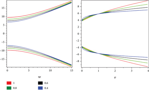
We have given simulation of problem 1 at different noninteger order (0 < ρ ≤ 1) for lower and upper portions of fuzzy solutions given in Figure 1 in two-dimensional form, respectively. The two similar color legends show the lower and upper branches of fuzzy solutions, respectively.

Example 2. Consider the fractional fuzzy biological population model

(42)

with the fuzzy initial condition

(43)

where

. Applying the abovementioned methodology as expressed (33), we achieved the following solutions.

(44)

We can write the series form solution

(45)

such that

(46)

In general, we can write as follows:

(47)

The exact result is

(48)

Details are in the caption following the image — **Figure 1**
Open in figure viewer PowerPoint

(a) A two-dimensional fuzzy upper and lower branch graph of an analytical series solution. (b) Different fractions of ρ.

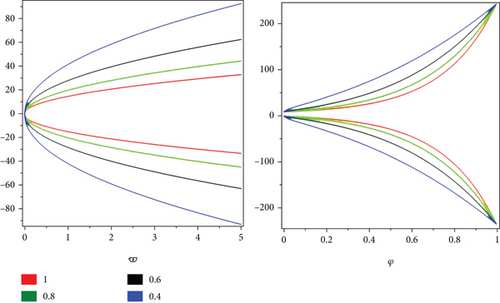
We have given simulation of problem 2 at different noninteger order (0 < ρ ≤ 1) for lower and upper portions of fuzzy solutions given in Figure 2 in two-dimensional form, respectively. The two similar color legends show the lower and upper branches of fuzzy solutions, respectively.

Example 3. Consider the fractional fuzzy biological population model

(49)

with the fuzzy initial condition

(50)

where

. Applying the above-mentioned procedure as expressed in (33), we achieved the following solutions.

(51)

We can write the series form solution

(52)

such that

(53)

In general, we can write as follows:

(54)

The exact result is

(55)

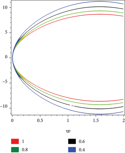
We have given simulation of problem 3 at different noninteger order (0 < ϱ ≤ 1) for lower and upper portions of fuzzy solutions given in Figure 3 in two-dimensional form, respectively. The two similar color legends show the lower and upper branches of fuzzy solutions, respectively.

4. Conclusion

In this paper, a concept of fuzzy Caputo fractional derivative was employed and introduced to analysis solutions of fuzzy biological population equations. An important example validated the conclusion reached. Additionally, we supplied graphs of the numerical solution in a variety of fractional order. Moreover, a technique was suggested to analysis results of fuzzy biological population equations in sense of Caputo operator. As a result, some concrete applications are shown to validate the theoretical framework based on the fuzzy Caputo calculus. Using this notion, we confirm that the proposed study can be used effectively as an extended planner in dealing with many sorts of uncertain situations in engineering and applied mathematics. To summarize, obtaining analytical solutions for many forms of fuzzy fractional differential equations is difficult. As a result, future studies must focus on analyzing and solving fractional fuzzy integro differential equations and fractional fuzzy dynamical systems based on the different derivative of fractional order ρ.

Conflicts of Interest

The authors declare that there are no conflicts of interest regarding the publication of this article.

Open Research

Data Availability

The numerical data used to support the findings of this study are included within the article.

References

1 Alaoui M. K., Fayyaz R., Khan A., and Abdo M. S., Analytical investigation of Noyes–Field model for time-fractional Belousov–Zhabotinsky reaction, Complexity. (2021) 2021, 21, https://doi.org/10.1155/2021/3248376, 3248376.
10.1155/2021/3248376
Web of Science® Google Scholar
2 Nonlaopon K., Naeem M., Zidan A. M., Alsanad A., and Gumaei A., Numerical investigation of the time-fractional Whitham–Broer–Kaup equation involving without singular kernel operators, Complexity. (2021) 2021, 21, https://doi.org/10.1155/2021/7979365, 7979365.
10.1155/2021/7979365
Web of Science® Google Scholar
3 Sunthrayuth P., Aljahdaly N. H., Ali A., and Tchalla A. M., Φ-Haar wavelet operational matrix method for fractional relaxation-oscillation equations containing Φ-Caputo fractional derivative, Journal of Function Spaces. (2021) 2021, 14, https://doi.org/10.1155/2021/7117064, 7117064.
10.1155/2021/7117064
Web of Science® Google Scholar
4 Agarwal R. P., Lakshmikantham V., and Nieto J. J., On the concept of solution for fractional differential equations with uncertainty, Nonlinear Analysis: Theory Methods & Applications. (2010) 72, no. 6, 2859–2862, https://doi.org/10.1016/j.na.2009.11.029, 2-s2.0-73249139676.
10.1016/j.na.2009.11.029
Web of Science® Google Scholar
5 Bhaskara T. G., Lakshmikanthama V., and Leela S., Fractional differential equations with a Krasnoselskii-Krein type condition, Nonlinear Analysis: Hybrid Systems. (2009) 3, no. 4, 734–737, https://doi.org/10.1016/j.nahs.2009.06.010, 2-s2.0-68749089513.
10.1016/j.nahs.2009.06.010
Web of Science® Google Scholar
6 Kilbas A. A., Srivastava M. H., and Trujillo J. J., Theory and Application of Fractional Differential Equations, 2006, Elsevier, Amsterdam, The Netherlands.
Google Scholar
7 Miller K. S. and Ross B., An Introduction to the Fractional Calculus and Fractional Diffrential Equations, 1993, John Wiley and Sons, New York, NY, USA.
Google Scholar
8 Shah N. A., Alyousef H. A., El-Tantawy S. A., Shah R., and Chung J. D., Analytical investigation of fractional-order Korteweg-De-Vries-type equations under Atangana-Baleanu-Caputo operator: modeling nonlinear waves in a plasma and fluid, Symmetry. (2022) 14, no. 4, https://doi.org/10.3390/sym14040739.
10.3390/sym14040739
Google Scholar
9 Noeiaghdam Z., Allahviranloo T., and Nieto J. J., Q-fractional differential equations with uncertainty, Soft Computing. (2019) 23, no. 19, 9507–9524, https://doi.org/10.1007/s00500-019-03830-w, 2-s2.0-85062679470.
10.1007/s00500-019-03830-w
Web of Science® Google Scholar
10 Ngo V. H., Fuzzy fractional functional integral and differential equations, Fuzzy Sets and Systems. (2015) 280, 58–90, https://doi.org/10.1016/j.fss.2015.01.009, 2-s2.0-84941878741.
10.1016/j.fss.2015.01.009
Web of Science® Google Scholar
11 Allahviranloo T., Uncertain information and linear systems, Studies in Systems, Decision and Control, 2020, 254, Springer, Berlin/Heidelberg, Germany, 109–119.
Google Scholar
12 Allahviranloo T., Gouyandeh Z., and Armand A., A full fuzzy method for solving differential equation based on Taylor expansion, Journal of Intelligent Fuzzy Systems. (2015) 29, no. 3, 1039–1055, https://doi.org/10.3233/IFS-151713, 2-s2.0-84944533871.
10.3233/IFS-151713
Web of Science® Google Scholar
13 Chehlabi M. and Allahviranloo T., Concreted solutions to fuzzy linear fractional differential equations, Applied Soft Computing. (2016) 44, 108–116, https://doi.org/10.1016/j.asoc.2016.03.011, 2-s2.0-84963540035.
10.1016/j.asoc.2016.03.011
Web of Science® Google Scholar
14 Hoa N. V., Fuzzy fractional functional differential equations under Caputo gH- differentiability, Communications in Nonlinear Science and Numerical Simulation. (2015) 22, no. 1-3, 1134–1157, https://doi.org/10.1016/j.cnsns.2014.08.006, 2-s2.0-84916631378.
10.1016/j.cnsns.2014.08.006
Web of Science® Google Scholar
15 Agarwal R. P., Baleanu D., Nieto J. J., Torres D. F. M., and Zhou Y., A survey on fuzzy fractional differential and optimal control nonlocal evolution equations, Journal of Computational and Applied Mathematics. (2018) 339, 3–29, https://doi.org/10.1016/j.cam.2017.09.039, 2-s2.0-85031405471.
10.1016/j.cam.2017.09.039
Web of Science® Google Scholar
16 Long H. V., Son N. T. K., and Tam H. T. T., The solvability of fuzzy fractional partial differential equations under Caputo gH-differentiability, Fuzzy Sets and Systems. (2017) 309, 35–63, https://doi.org/10.1016/j.fss.2016.06.018, 2-s2.0-85004093030.
10.1016/j.fss.2016.06.018
Web of Science® Google Scholar
17 Salahshour S., Allahviranloo T., and Abbasbandy S., Solving fuzzy fractional differential equations by fuzzy Laplace transforms, Communications in Nonlinear Science and Numerical Simulation. (2012) 17, no. 3, 1372–1381, https://doi.org/10.1016/j.cnsns.2011.07.005, 2-s2.0-80053384834.
10.1016/j.cnsns.2011.07.005
Web of Science® Google Scholar
18 Alesemi M., Iqbal N., and Wyal N., Novel evaluation of fuzzy fractional helmholtz equations, Journal of Function Spaces. (2022) 2022, article 8165019.
Web of Science® Google Scholar
19 Iqbal N., Niazi A. U. K., Khan I. U., and Botmart T., Cauchy problem for non-autonomous fractional evolution equations with nonlocal conditions of order (1, 2), AIMS Mathematics. (2022) 7, no. 5, 8891–8913, https://doi.org/10.3934/math.2022496.
10.3934/math.2022496
Web of Science® Google Scholar
20 Mukhtar S., Shah R., and Noor S., The numerical investigation of a fractional-order multi-dimensional model of Navier-Stokes equation via novel techniques, Symmetry. (2022) 14, no. 6, https://doi.org/10.3390/sym14061102.
10.3390/sym14061102
Web of Science® Google Scholar
21 Gurtin M. E. and MacCamy R. C., On the diffusion of biological populations, Mathematical Biosciences. (1977) 33, no. 1-2, 35–49, https://doi.org/10.1016/0025-5564(77)90062-1, 2-s2.0-0017357730.
10.1016/0025-5564(77)90062-1
Web of Science® Google Scholar
22 Zhang L. W., Deng Y. J., and Liew K. M., An improved element-free Galerkin method for numerical modeling of the biological population problems, Engineering Analysis with Boundary Elements. (2014) 40, 181–188, https://doi.org/10.1016/j.enganabound.2013.12.008, 2-s2.0-84892962543.
10.1016/j.enganabound.2013.12.008
Web of Science® Google Scholar
23 Gurney W. S. C. and Nisbet R. M., The regulation of inhomogeneous populations, Journal of Theoretical Biology. (1975) 52, no. 2, 441–457, https://doi.org/10.1016/0022-5193(75)90011-9, 2-s2.0-0016753474, 1195750.
10.1016/0022-5193(75)90011-9
CAS PubMed Web of Science® Google Scholar
24 Ojo G. O. and Mahmudov N. I., Aboodh transform iterative method for spatial diffusion of a biological population with fractional-order, Mathematics. (2021) 9, no. 2, https://doi.org/10.3390/math9020155.
10.3390/math9020155
Web of Science® Google Scholar
25 Yavuz M. and Ozdemir N., Analysis of an epidemic spreading model with exponential decay law, Mathematical Sciences and Applications E-Notes. (2020) 8, no. 1, 142–154, https://doi.org/10.36753/mathenot.691638.
10.36753/mathenot.691638
Google Scholar
26 Iqbal N., Akgul A., Bariq A., Mossa Al-Sawalha M., and Ali A., On solutions of fractional-order gas dynamics equation by effective techniques, Journal of Function Spaces. (2022) 2022, 14, https://doi.org/10.1155/2022/3341754, 3341754.
10.1155/2022/3341754
Web of Science® Google Scholar
27 Bear J. and Braester C., On the flow of two immscible fluids in fractured porous media, Developments in Soil Science, 1972, Elsevier, 177–202, https://doi.org/10.1016/S0166-2481(08)70538-5, 2-s2.0-62949130935.
Google Scholar
28 Yasmin H. and Iqbal N., Convective mass/heat analysis of an electroosmotic peristaltic flow of ionic liquid in a symmetric porous microchannel with soret and dufour, Mathematical Problems in Engineering. (2021) 2021, 14, 2638647, https://doi.org/10.1155/2021/2638647.
10.1155/2021/2638647
Web of Science® Google Scholar
29 Adomian G., A new approach to nonlinear partial differential equations, Journal of Mathematical Analysis and Applications. (1984) 102, no. 2, 420–434, https://doi.org/10.1016/0022-247X(84)90182-3, 2-s2.0-0021495016.
10.1016/0022-247X(84)90182-3
Web of Science® Google Scholar
30 Rawashdeh M. S. and Al-Jammal H., New approximate solutions to fractional nonlinear systems of partial differential equations using the FNDM, Advances in Difference Equations. (2016) 2016, no. 1, https://doi.org/10.1186/s13662-016-0960-x, 2-s2.0-84987896411.
10.1186/s13662-016-0960-x
Google Scholar
31 Rawashdeh M. S. and Al-Jammal H., Numerical solutions for systems of nonlinear fractional ordinary differential equations using the FNDM, Mediterranean Journal of Mathematics. (2016) 13, no. 6, 4661–4677, https://doi.org/10.1007/s00009-016-0768-7, 2-s2.0-84977151023.
10.1007/s00009-016-0768-7
Web of Science® Google Scholar
32 Prakasha D. G., Veeresha P., and Rawashdeh M. S., Numerical solution for (2 + 1)-dimensional time-fractional coupled Burger equations using fractional natural decomposition method, Mathematical Methods in the Applied Sciences. (2019) 42, no. 10, 3409–3427, https://doi.org/10.1002/mma.5533, 2-s2.0-85063887395.
10.1002/mma.5533
Web of Science® Google Scholar
33 Prakasha D. G., Veeresha P., and Baskonus H. M., Two novel computational techniques for fractional Gardner and Cahn-Hilliard equations, Computational and Mathematical Methods. (2019) 1, no. 2, article e1021, https://doi.org/10.1002/cmm4.1021.
10.1002/cmm4.1021
Google Scholar
34 Shakeri F. and Dehghan M., Numerical solution of a biological population model using He’s variational iteration method, Computers & Mathematics with Applications. (2007) 54, no. 7-8, 1197–1209, https://doi.org/10.1016/j.camwa.2006.12.076, 2-s2.0-34848823089.
10.1016/j.camwa.2006.12.076
Web of Science® Google Scholar
35 Roul P., Application of homotopy perturbation method to biological population model, Applications and Applied Mathematics: An International Journal (AAM). (2010) 5, no. 2.
Google Scholar
36 Kumar S. and Kumar D., Fractional modelling for BBM-Burger equation by using new homotopy analysis transform method, Journal of the Association of Arab Universities for Basic and Applied Sciences. (2014) 16, no. 1, 16–20, https://doi.org/10.1016/j.jaubas.2013.10.002, 2-s2.0-84908024874.
10.1016/j.jaubas.2013.10.002
Google Scholar
37 Allahviranloo T. and Ahmadi M. B., Fuzzy laplace transforms, Soft Computing. (2010) 14, no. 3, 235–243, https://doi.org/10.1007/s00500-008-0397-6, 2-s2.0-70350649223.
10.1007/s00500-008-0397-6
Web of Science® Google Scholar

Citing Literature

All articles

Novel Evaluation of Fuzzy Fractional Biological Population Model

Abstract

1. Introduction

2. Basic Definitions

3. Road Map of the Current Method

3.1. Numerical Results

4. Conclusion

Conflicts of Interest

Open Research

Data Availability

References

Citing Literature

Figures

References

Information

About Wiley Online Library

Help & Support

Opportunities

Connect with Wiley

Novel Evaluation of Fuzzy Fractional Biological Population Model

Abstract

1. Introduction

2. Basic Definitions

3. Road Map of the Current Method

3.1. Numerical Results

4. Conclusion

Conflicts of Interest

Open Research

Data Availability

References

Citing Literature

Figures

References

Related

Information