Volume 2022, Issue 1 3666348

Research Article

Open Access

Numerical and Analytical Simulations of Nonlinear Time Fractional Advection and Burger’s Equations

Hassan Khan,

Corresponding Author

Hassan Khan

[email protected]

orcid.org/0000-0001-6417-1181

Department of Mathematics, Abdul Wali Khan University Mardan, Pakistan awkum.edu.pk

Department of Mathematics, Near East University TRNC, Mersin 10, Turkey neu.edu.tr

Search for more papers by this author

Qasim Khan,

Qasim Khan

orcid.org/0000-0002-7572-1393

Department of Mathematics, Abdul Wali Khan University Mardan, Pakistan awkum.edu.pk

Department of Mathematics and Information Technology, The Education University of Hong Kong, 10 Lo Ping Road, Tai Po, New Territories, Hong Kong ied.edu.hk

Search for more papers by this author

Fairouz Tchier,

Fairouz Tchier

orcid.org/0000-0001-7855-508X

Department of Mathematics, College of Science, King Saud University, P.O. Box 2455, Riyadh 11451, Saudi Arabia ksu.edu.sa

Search for more papers by this author

Ibrarullah,

Ibrarullah

Department of Mathematics, Abdul Wali Khan University Mardan, Pakistan awkum.edu.pk

Search for more papers by this author

Evren Hincal,

Evren Hincal

orcid.org/0000-0001-6175-1455

Department of Mathematics, Near East University TRNC, Mersin 10, Turkey neu.edu.tr

Search for more papers by this author

Gurpreet Singh,

Gurpreet Singh

orcid.org/0000-0003-2961-9379

School of Mathematical Sciences, Dublin City University, Ireland dcu.ie

Search for more papers by this author

F. M. O. Tawfiq,

F. M. O. Tawfiq

Department of Mathematics, College of Science, King Saud University, P.O. Box 2455, Riyadh 11451, Saudi Arabia ksu.edu.sa

Search for more papers by this author

Shahbaz Khan,

Shahbaz Khan

orcid.org/0000-0003-3661-3303

Department of Mathematics, Abdul Wali Khan University Mardan, Pakistan awkum.edu.pk

Search for more papers by this author

Hassan Khan,

Corresponding Author

Hassan Khan

[email protected]

orcid.org/0000-0001-6417-1181

Department of Mathematics, Abdul Wali Khan University Mardan, Pakistan awkum.edu.pk

Department of Mathematics, Near East University TRNC, Mersin 10, Turkey neu.edu.tr

Search for more papers by this author

Qasim Khan,

Qasim Khan

orcid.org/0000-0002-7572-1393

Department of Mathematics, Abdul Wali Khan University Mardan, Pakistan awkum.edu.pk

Department of Mathematics and Information Technology, The Education University of Hong Kong, 10 Lo Ping Road, Tai Po, New Territories, Hong Kong ied.edu.hk

Search for more papers by this author

Fairouz Tchier,

Fairouz Tchier

orcid.org/0000-0001-7855-508X

Department of Mathematics, College of Science, King Saud University, P.O. Box 2455, Riyadh 11451, Saudi Arabia ksu.edu.sa

Search for more papers by this author

Ibrarullah,

Ibrarullah

Department of Mathematics, Abdul Wali Khan University Mardan, Pakistan awkum.edu.pk

Search for more papers by this author

Evren Hincal,

Evren Hincal

orcid.org/0000-0001-6175-1455

Department of Mathematics, Near East University TRNC, Mersin 10, Turkey neu.edu.tr

Search for more papers by this author

Gurpreet Singh,

Gurpreet Singh

orcid.org/0000-0003-2961-9379

School of Mathematical Sciences, Dublin City University, Ireland dcu.ie

Search for more papers by this author

F. M. O. Tawfiq,

F. M. O. Tawfiq

Department of Mathematics, College of Science, King Saud University, P.O. Box 2455, Riyadh 11451, Saudi Arabia ksu.edu.sa

Search for more papers by this author

Shahbaz Khan,

Shahbaz Khan

orcid.org/0000-0003-3661-3303

Department of Mathematics, Abdul Wali Khan University Mardan, Pakistan awkum.edu.pk

Search for more papers by this author

First published: 06 October 2022

https://doi.org/10.1155/2022/3666348

Citations: 1

Academic Editor: Yusuf Gurefe

Share a link

Email
Wechat
Bluesky

Abstract

In this paper, the higher nonlinear problems of fractional advection-diffusion equations and systems of nonlinear fractional Burger’s equations are solved by using two sophisticated procedures, namely, the q-homotopy analysis transform method and the residual power series method. The proposed methods are implemented with the Caputo operator. The present techniques are utilised in a very comprehensive and effective manner to obtain the solutions to the suggested fractional-order problems. The nonlinearity of the problem was controlled tactfully. The numerical results of a few examples are calculated and analyzed. The tables and graphs are constructed to understand the higher accuracy and applicability of the current method. The obtained results that are in good contact with the actual dynamics of the given problem, which is verified by the graphs and tables. The present techniques require fewer calculations and are associated with a higher degree of accuracy, and therefore can be extended to solve other high nonlinear fractional problems.

1. Introduction

The most powerful tool for researchers to simulate various physical phenomena in applied sciences and nature is known as fractional partial differential equations (FPDEs). The following physical phenomena have been accurately modelled by FPDEs: optics [1], economics [2], fluid traffic [3], electrodynamics [4], hepatitis B virus [5], tuberculosis [6], air foil [7], modelling of earth quack nonlinear oscillation [8], propagation of spherical waves [9], Chaos theory [10], fractional COVID-19 model [11], finance [12], pine wilt disease [13], Zener [14], cancer chemotherapy [15], traffic flow model [16], Poisson-Nernst-Planck diffusion [17], diabetes [18], biomedical and biological [19], and many other numerous applications in various branches of applied mathematics (see [20–22]). Due to these numerous applications, FPDEs and factional calculus have gained more attention from researchers as compared to ordinary calculus.

To obtain the approximate solutions to the above models, researchers use and develop a variety of analytical approaches. The frequently used methods are optimal homotopy asymptotic method (OHAM) [23], Iterative Laplace transform method [24], extended direct algebraic method (EDAM) [25], Adomian decomposition method (ADM) [26], the Finite difference method (FDM) [27], the homotopy perturbation transform technique along with transformation (HPTM) [28], the (G/G^′)-expansion method [29], the Haar wavelet method (HWM) [30], standard reductive perturbation method [31], the variational iteration procedure with transformation (VITM) [32], and the differential transform method (DTM) [33]. In this context, Hassan et al. have presented the solutions of some nonlinear FPDEs which can be seen in [34–36]. Some useful methods can be seen in [37–39].

Obtaining the analytical solutions of FPDEs and their systems has been a difficult task for researchers in recent years. In this circumstance, Prakash and Kaur use q-HATM [40] to solve the time-fractional Navier Stokes equation. Similarly, q-HATM was implemented by Kumar et al. and used to obtain the solutions of the fractional long-wave equations in the regularised form [41]. The Schrodinger generalized form of fractional order was solved by Veeresha et al. using q-HATM [42]. The q-HATM convergence was done by El-Tawil and Huseen [43]. The RPSM technique was used by Alquran to solve the drainage equation in [44] and the fractional-order Phi-4 equation in [45]. The Whitham-Broer-Kaup equation of fractional order was analysed by Wang and Chen by using RPSM [46]. RPSM has been used in [47] to find the solution of the fractional Biswas-Milovic equation of multidimensions. Komashynska et al. used the RPSM [48] to solve a system of multipantograph delay differential equations. In [49], RPSM was used to find an approximation solution for the fractional-order Sharma-Tasso-Olever equation. The solutions to the fractional order Schrodinger equations were determined using RPSM in [50]. The RPSM has been used to solve a variety of problems, including the gas dynamic equation [51], the Emden-Fowler equation, Berger-Fisher equation, and the Benney-Lin equation in its fractional format, solved by RPSM in [52]. Similarly, RPSM was used by Al-Smadi [53] to overcome the solutions to initial value problems.

In this paper, the solutions of systems of fractional Berger’s equations and nonlinear advection equations were examined by combining two analytical techniques, q-HAM and RPSM. The results are compared to each other as well as the exact solution to the given problems. The current methods are used to compare the solutions methodologies for the analysis of the higher nonlinear problems of fractional advection-diffusion equations and systems of nonlinear fractional Burger’s equations in the Caputo sense. The obtained approximate series solutions are fast converging towards the exact solutions of the targeted problems, according to quantitative analysis. It is found that the techniques under discussion are simple and effective for the solutions of FPDE systems. The graphs and tables for the solutions to the targeted problems via RPSM and q-HATM. It is confirmed that the obtained solutions are in good contact with the exact solution to the problems. The fractional order solutions are convergent towards the integer order solutions, which shows the reliability of the fractional solutions. The presented techniques have a wide range of applications and could be used to examine approximate analytical solutions of other nonlinear FPDEs and multidimensional systems of FPDEs in the future.

This paper will be formatted as follows: in the second section, some basic definitions are discussed. In Section 3, the methodology is described, and in Section 4, two separate techniques are used to compare certain numerical results. The conclusion and references are found in the fifth and final section of the paper.

2. Basic Definitions

In this section we will discuss some important definitions

2.1. Definition

The Caputo operator in [54, 55] is given as.

(1)

2.2. Definition

An expansion of power series (PS) at point t = t₀ is known as fractional PS and is given by [56].

(2)

note FPS can be expanded at point t₀ is

(3)

which is the Taylor’s series expansion form.

2.3. Laplace Transform (LT)

The LT for continuous function

is defined as [57]

(4)

where G(s) is the LT for the function

2.4. Definition

The LT

of Caputo fractional derivative is given by [57]

(5)

2.5. Definition

The LT of two function

is defined by [57]

(6)

, represent the product between k and

(7)

2.6. Definition

The LT of fractional derivative is defined as [57]

(8)

where the LT of

is denoted by G(s).

2.7. Theorem

Assume that the series solution

is convergent to the solution u for a prescribed value of h. If the truncated series

(9)

is used as an approximation to the solution u(x, t) of problem, then an upper bound for the error, E_m is estimated as

(10)

Proof. See [43]

2.8. Theorem

suppose that u(t) ∈ C[t₀, t₀ + R] and fork = 0, 1, 2, ⋯, n + 1,

where 0 < α ≤ 1. Then u could be represented by:

(11)

Proof. See [58].

2.9. Theorem

on t₀ ≤ t ≤ d, where 0 < α ≤ 1, then the reminder R_n(t) of the generalized Taylor’s series will satisfies the inequality:

(12)

Proof. See [58].

2.10. Theorem

Suppose that u has a Fractional power series representation at t₀ of the form

(13)

where R is the radius of convergence. Then u is analytic in (t₀, t₀ + R).

Proof. See [58].

3. RPSM and Q-HATM Procedures

To understand main concept of RPSM and q-HATM [59] for system of FPDEs, we consider the following FPDEs system,

(14)

with initial condition,

(15)

where

the Caputo fractional derivative, R is linear and N is nonlinear operator, respectively, in Eq. (14).

3.1. RPSM Procedure for FPDEs System [60]

Eq. (14) can be simplified as

(16)

where υ(x, y, z, t), ϑ(x, y, z, t), and ϖ(x, y, z, t) is the k^th truncated series of form

(17)

In RPSM the zero^th approximate solution of υ(x, y, z, t), ϑ(x, y, z, t), and ϖ(x, y, z, t) is given by

(18)

Eq. (17), implies that,

(19)

for Eq. (14), the residual function is given by

(20)

so, the k^th residual function becomes

(21)

As in [61, 62], it is clear that Res(x, y, z, t) = 0 and . Therefore, , , and . In the Caputo definition, the constant has zero derivative therefore , k = 0, 1, ⋯, n which mean that of Res_υ(x, y, z, t), Res_ϑ(x, y, z, t), Res_ϖ(x, y, z, t), and Res_k(x, y, z, t) are t = 0 matching at n = 0, 1, ⋯, k; .

To determine f₁(x, y, z), f₂(x, y, z), f₃(x, y, z), ⋯, g₁(x, y, z), g₂(x, y, z), g₃(x, y, z), ⋯, and h₁(x, y, z), h₂(x, y, z), h₃(x, y, z), ⋯, we substitute k = 0, 1, ⋯, in Eq. (17), and then the obtained results are put in Eq. (19). In the final step, we apply

on both sides we obtained the following

(22)

3.2. Q-HATM Procedure for FPDEs System [63]

Using LT, Eq. (14) can be simplified as

(23)

so Eq. (23), implies that

(24)

We define the nonlinear operator is

(25)

where q ∈ [0, (1/n)], θ(x, y, z, t; q) is real function of x, y, z, t, and q.

Homotopy can be constructed as

(26)

In Eq. (26), the auxiliary parameter, nonzero auxiliary function and embedding parameter are h ≠ 0, H(x, y, z, t) and n ≥ 1, q ∈ [0, (1/n)], respectively.

denotes Laplacian operator and υ₀, ϑ₀, and ϖ₀ are the initial conditions. The following results are obtained at q = 0 and q = 1/n,

(27)

By using Taylor theorem θ(x, y, z, t; q) can be expressed as

(28)

where

(29)

After simplification, we have

(30)

Taking the m-times derivatives of Eq. (26), put q = 0, implies the zero^th order solution

(31)

where the vectors are defined as

(32)

The following recursive formula is obtained by taking inverse LT of Eq. (31),

(33)

Where

(34)

(35)

Eq. (33) and Eq. (35) are known q-HATM series solutions for the given system.

4. Numerical Results

4.1. Example

Consider nonlinear advection-diffusion equation of the form [64]

(36)

with ICs

(37)

and exact solution at δ = 1

(38)

4.1.1. RPSM-Solution

(1) 1st Iteration. Using RPSM, the k^th truncated series of Eq. (36), can obtain

(39)

the 1st approximate is given as

(40)

Eq. (39) should be written as

(41)

put k = 1 in Eq. (41), we get

(42)

where υ(x, 0) = f(x) = e^−x,

(43)

The residual function of Eq. (36), is given by

(44)

The k^th residual function Resυ(x, t) is given by,

(45)

put k = 1 in the Eq. (45), we obtain

(46)

we have

(47)

Eq. (46), will become

(48)

(2) 2nd Iteration. for k = 2 Eq. (41), can be written as

(49)

where f(x) = e^−x, and f₁(x) = e^−x,

(50)

put k = 2 in Eq. (45), we obtain

(51)

(52)

as we know that

(53)

for k = 2 Eq. (53), become as

(54)

using

on Eq. (52), we get

(55)

put

in Eq. (55), we obtain

(56)

(3) 3rd Iteration. Put k = 3 in Eq. (41), we obtain

(57)

where f(x) = e^−x, f₁(x) = e^−x, and f₂(x) = e^−x,

(58)

put k = 3 in Eq. (45) we obtain

(59)

(60)

put k = 3 in Eq. (53), we obtain

(61)

applying

on both sides of the Eq. (60), we get

(62)

put

in Eq. (62), we obtain

(63)

The RPSM solution of Eq. (36), is given as

(64)

4.1.2. Q-HATM Solution

(1) 1st Iteration. Taking LT of Eq. (36), and simplifying

(65)

The nonlinear term N is defined as

(66)

Using the procedure of q-HATM

(67)

put m = 1 in the Eq. (67), we obtain

(68)

(69)

put m = 1 in Eq. (69), we obtain

(70)

put in Eq. (68), we obtain

(71)

(2) 2nd Iteration. Put m = 2 in the Eq. (67), we obtain

(72)

put m = 2 in Eq. (69), we obtain

(73)

put in Eq. (72), we obtain

(74)

(3) 3rd Iteration. Put m = 3 in the Eq. (67), we obtain

(75)

put m = 3 in Eq. (69), we obtain

(76)

put in Eq. (75), we obtain

(77)

The q-HATM solution of Eq. (36), is given as

(78)

4.2. Example

The system of 3D Burgers’ equation are [65, 66]

(79)

the initial condition of Eq. (79), are

(80)

The exact solution of the Eq. (79) at δ = 1, are

(81)

4.2.1. RPSM-Solution

(1) 1st Iteration. The k^th truncated series of the solution of Eq. (79), using RPSM, we obtain

(82)

the zero^th RPSM approximate solution of Eq. (79), is given by

(83)

the Eq. (82), should be written as

(84)

put k = 1 in Eq. (84), we get

(85)

where

(86)

The residual function of Eq. (79), is given by

(87)

where the k^th residual function of Resυ(x, y, t), Resϑ(x, y, t), and Resϖ(x, y, t) is given by

(88)

put k = 1 in the Eq. (88), we obtain

(89)

(90)

we know that

(91)

put in Eq. (90), we obtain

(92)

(2) 2nd Iteration. Put k = 2 in Eq. (84), we obtain

(93)

where

(94)

put k = 2 in the Eq. (88), we obtain

(95)

(96)

we know that

(97)

put k = 2 in Eq. (97), we obtain

(98)

applying

, on both sides of the Eq. (96), we get

(99)

we know that

(100)

put in Eq. (99), we obtain

(101)

The solution of Eq. (79), in term of RPSM is given by

(102)

4.2.2. Q-HATM Solution

(1) 1st Iteration. Taking LT of Eq. (79), and simplifying we obtain

(103)

The nonlinear term N is defined as

(104)

Use the procedure of q-HATM

(105)

put m = 1 in the Eq. (105), we obtain

(106)

(107)

put m = 1 in Eq. (107), we get

(108)

Put in Eq. (106), we obtain

(109)

(2) 2nd Iteration. Put m = 2 in the Eq. (105), we obtain

(110)

put m = 2 in Eq. (107), we obtain

(111)

after simplification we obtain

(112)

Put Eq. (112) in Eq. (110), we obtain

(113)

The solution of Eq. (79), in term of q-HATM is given by

(114)

5. Results and Discussion

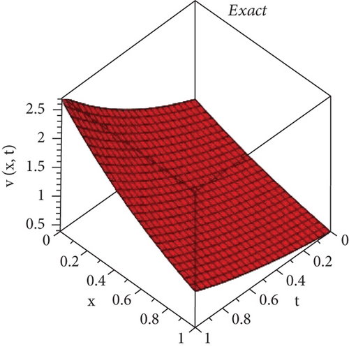
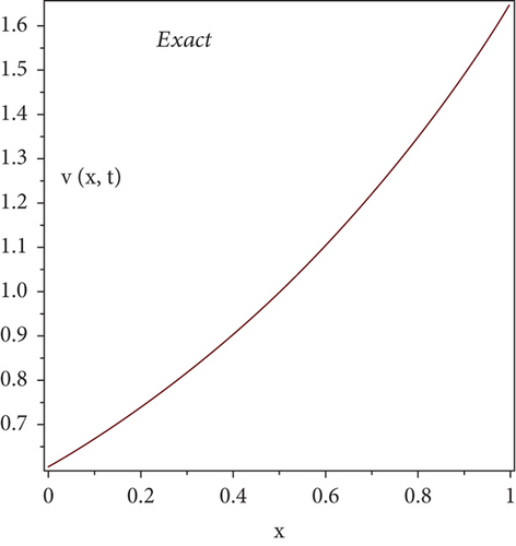
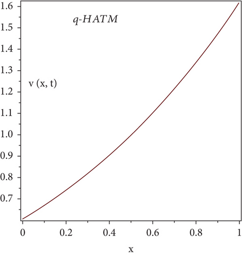
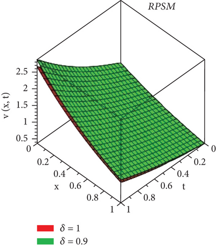
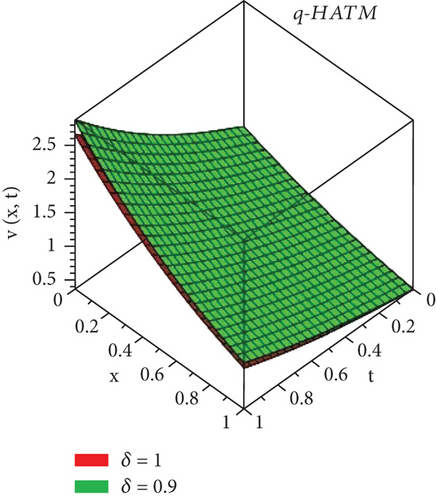
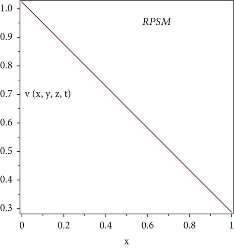
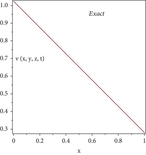
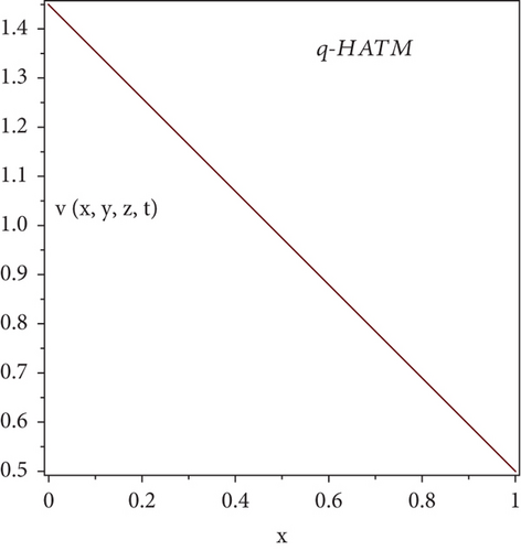
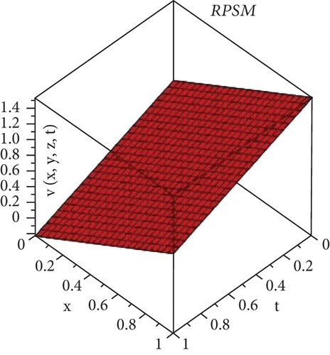
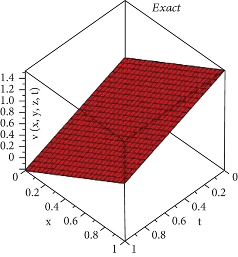
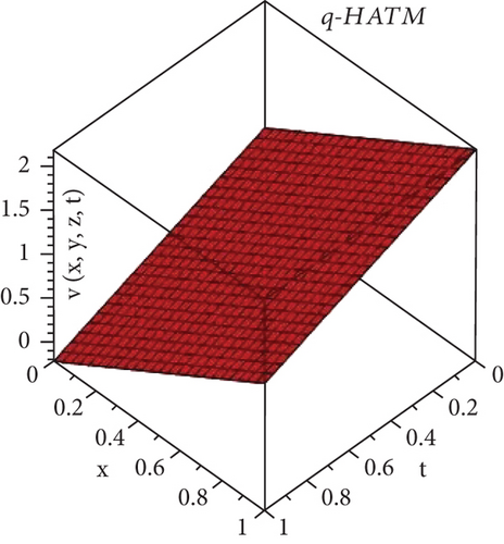
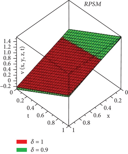
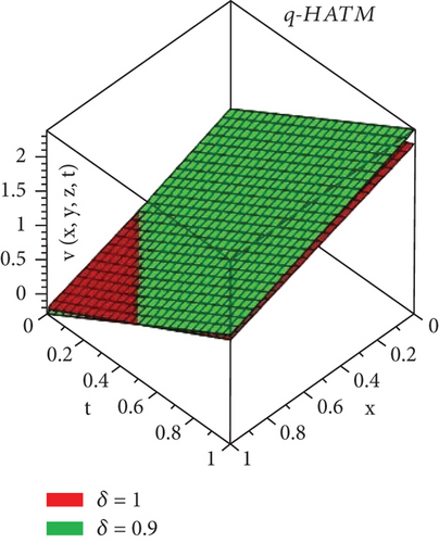
Here, we will discuss the numerical solutions. In Figure 1, 3D plots of (a) RPSM, (b) Exact, and (c) q-HATM ψ−solutions at δ = 1 of Example 4.1 are presented. Which are in closed contact with the exact solution of Example 4.1. In Figure 2, 2D plots of (a) RPSM, (b) Exact, and (c) q-HATM ψ−solutions at δ = 1 of Example 4.1 are presented, from which the validity of the proposed methods are confirmed. While in Figure 3, 3D plots of Example 4.1 for fractional order δ = 1,0.9 are plotted. Numerical values of Example 4.1 are presented in Table 1. In Figure 4, 2D-solutions plots and Figure 5 of (a) RPSM, (b) Exact, and (c) q-HATM, at δ = 1 of Example 4.2 are plotted. The RPSM and q-HATM solutions are very closed to the exact solution. The RPSM and q-HATM solutions graphs at different fractional order are plotted in Figure 6.

Details are in the caption following the image — **Figure 1 (a)**
Open in figure viewer PowerPoint

3D plots of (a) RPSM, (b) Exact, and (c) q-HATM υ−solutions at δ = 1 of Example 4.1.

Table 1. Solution comparison of RPSM, q-HATM, and Exact with different time and spaces of Example 4.1.

x	t	RPSM	RPSM	q-HATM	q-HATM	Exact
x	t	δ = 0.9	δ = 1	δ = 0.9	δ = 1	δ = 1
0.25	0.001	0.7804183	0.7795799	0.7804183	0.7795799	0.7795799
0.50		0.6077903	0.6071374	0.6077903	0.6071374	0.6071374
0.75		0.4733476	0.4728391	0.4733476	0.4728391	0.4728391
1		0.3686435	0.3682475	0.3686435	0.3682475	0.3682475
0.25	0.005	0.7857118	0.7827045	0.7857118	0.7827045	0.7827045
0.50		0.6119130	0.6095709	0.6119130	0.6095709	0.6095709
0.75		0.4765583	0.4747342	0.4765583	0.4747342	0.4747342
1		0.3711440	0.3697234	0.3711440	0.3697234	0.3697234

6. Conclusion

In this paper, the solutions of nonlinear systems of fractional Burger’s equations and advection diffusion equation are calculated by using q-HATM and RPSM. The proposed methods provide the results with higher degree of accuracy and using very few terms of their series solutions. The solutions comparison of both techniques are compared with the actual solutions of each problem. The comparison has shown the best compromise between the solutions of the suggested techniques. The fractional-order solutions are calculated successfully and shown to be convergent towards the integer-order solutions. The novelty of this paper is given in the nonlinear fractional solutions which provide the more accurate results as compared to other studies in literature. In the future, the suggested techniques can be utilised easily for the solutions of higher dimensional and nonlinear FPDEs and their systems because of their simple and straightforward implementation.

Disclosure

This work is performed as part of the employment of the authors.

Conflicts of Interest

No competing interests are declared.

Authors’ Contributions

Hassan Khan was responsible for supervision, Qasim khan was responsible for methodology and draft writing, Fairouz Tchier was the project administrator, Ibrar Ullah was responsible for the methodology, Evren Hincal was responsible for funding and draft writing, Gurpreet Singh was responsible for draft writing, F. M. O. Tawfiq was responsible for the investigation, and Shahbaz Khan was responsible for the methodology and draft writing.

Acknowledgments

Researchers Supporting Project (no. RSP-2021/401), King Saud University, Riyadh, Saudi Arabia.

Open Research

Data Availability

No data were used to support this study.

References

1 Longhi S., Fractional Schrödinger equation in optics, Optics Letters. (2015) 40, no. 6, 1117–1120, https://doi.org/10.1364/OL.40.001117, 2-s2.0-84961872424.
10.1364/OL.40.001117
PubMed Web of Science® Google Scholar
2 Tarasov V. E., On history of mathematical economics: application of fractional calculus, Mathematics. (2019) 7, no. 6, https://doi.org/10.3390/math7060509, 2-s2.0-85066821676.
10.3390/math7060509
Web of Science® Google Scholar
3 He J. H., Homotopy perturbation technique, Computer Methods in Applied Mechanics and Engineering. (1999) 178, no. 3-4, 257–262, https://doi.org/10.1016/S0045-7825(99)00018-3, 2-s2.0-0032672778.
10.1016/S0045-7825(99)00018-3
Web of Science® Google Scholar
4 Nasrolahpour H., A note on fractional electrodynamics, Communications in Nonlinear Science and Numerical Simulation. (2013) 18, no. 9, 2589–2593, https://doi.org/10.1016/j.cnsns.2013.01.005, 2-s2.0-84878019304.
10.1016/j.cnsns.2013.01.005
Web of Science® Google Scholar
5 Ullah S., Khan M. A., and Farooq M., A new fractional model for the dynamics of the hepatitis B virus using the Caputo-Fabrizio derivative, The European Physical Journal Plus. (2018) 133, no. 6, 1–14, https://doi.org/10.1140/epjp/i2018-12072-4.
10.1140/epjp/i2018-12072-4
Web of Science® Google Scholar
6 Khan M. A., Ullah S., and Farooq M., A new fractional model for tuberculosis with relapse via Atangana-Baleanu derivative, Chaos, Solitons and Fractals. (2018) 116, 227–238, https://doi.org/10.1016/j.chaos.2018.09.039, 2-s2.0-85054022770.
10.1016/j.chaos.2018.09.039
Web of Science® Google Scholar
7 Mahmood S., Shah R., and Arif M., Laplace adomian decomposition method for multi dimensional time fractional model of Navier-Stokes equation, Symmetry. (2019) 11, no. 2, https://doi.org/10.3390/sym11020149, 2-s2.0-85061870755.
10.3390/sym11020149
Web of Science® Google Scholar
8 He J. H., Nonlinear oscillation with fractional derivative and its applications, International Conference on Vibrating Engineering. (1998) 98, 288–291.
Google Scholar
9 Fellah Z. E. A., Fellah M., Roncen R., Ongwen N. O., Ogam E., and Depollier C., Transient propagation of spherical waves in porous material: application of fractional calculus, Symmetry. (2022) 14, no. 2, https://doi.org/10.3390/sym14020233.
10.3390/sym14020233
Web of Science® Google Scholar
10 Wu X., Lai D., and Lu H., Generalized synchronization of the fractional-order chaos in weighted complex dynamical networks with nonidentical nodes, Nonlinear Dynamics. (2012) 69, no. 1-2, 667–683, https://doi.org/10.1007/s11071-011-0295-9, 2-s2.0-84861733446.
10.1007/s11071-011-0295-9
Web of Science® Google Scholar
11 Din A., Khan A., Zeb A., Sidi Ammi M. R., Tilioua M., and Torres D. F., Hybrid method for simulation of a fractional COVID-19 model with real case application, Axioms. (2021) 10, no. 4, https://doi.org/10.3390/axioms10040290.
10.3390/axioms10040290
Web of Science® Google Scholar
12 Momani S. and Odibat Z., Analytical solution of a time-fractional Navier-Stokes equation by Adomian decomposition method, Applied Mathematics and Computation. (2006) 177, no. 2, 488–494, https://doi.org/10.1016/j.amc.2005.11.025, 2-s2.0-33744981446.
10.1016/j.amc.2005.11.025
Web of Science® Google Scholar
13 Khan M. A., Ullah S., Okosun K. O., and Shah K., A fractional order pine wilt disease model with Caputo–Fabrizio derivative, Advances in Difference Equations. (2018) 2018, no. 1, https://doi.org/10.1186/s13662-018-1868-4, 2-s2.0-85056113369.
10.1186/s13662-018-1868-4
Google Scholar
14 Birajdar G. A., Numerical solution of time fractional Navier-stokes equation by discrete Adomian decomposition method, Nonlinear Engineering. (2014) 3, no. 1, 21–26, https://doi.org/10.1515/nleng-2012-0004.
10.1515/nleng-2012-0004
Google Scholar
15 Veeresha P., Prakasha D. G., and Baskonus H. M., New numerical surfaces to the mathematical model of cancer chemotherapy effect in Caputo fractional derivatives, Journal of Nonlinear Science. (2019) 29, no. 1, article 013119, https://doi.org/10.1063/1.5074099, 2-s2.0-85060137783.
10.1063/1.5074099
Google Scholar
16 Kang Y., Mao S., and Zhang Y., Fractional time-varying grey traffic flow model based on viscoelastic fluid and its application, Transportation Research Part B: Methodological. (2022) 157, 149–174, https://doi.org/10.1016/j.trb.2022.01.007.
10.1016/j.trb.2022.01.007
Web of Science® Google Scholar
17 Chaurasia V. B. L. and Kumar D., Solution of the time-fractional Navier–Stokes equation, General Mathematics Notes. (2011) 4, no. 2, 49–59.
Google Scholar
18 Singh J., Kumar D., and Baleanu D., On the analysis of fractional diabetes model with exponential law, Advances in Difference Equations. (2018) 2018, no. 1, 1–15, https://doi.org/10.1186/s13662-018-1680-1, 2-s2.0-85049368790.
10.1186/s13662-018-1680-1
CAS Web of Science® Google Scholar
19 Bertsias P., Kapoulea S., Psychalinos C., and Elwakil A. S., A collection of interdisciplinary applications of fractional-order circuits, Fractional Order Systems, 2022, Academic Press, 35–69, https://doi.org/10.1016/B978-0-12-824293-3.00007-7.
10.1016/B978-0-12-824293-3.00007-7
Google Scholar
20 R. Hilfer, Applications of Fractional Calculus in Physics, 2000, Orlando.
10.1142/3779
Google Scholar
21 Kilbas A. A., Srivastava H. M., and Trujillo J. J., Theory and applications of fractional differential equations, 2006, 204, Elsevier.
10.1016/S0304-0208(06)80001-0
Google Scholar
22 Das S., A note on fractional diffusion equations, Chaos, Solitons and Fractals. (2009) 42, no. 4, 2074–2079, https://doi.org/10.1016/j.chaos.2009.03.163, 2-s2.0-67651006181.
10.1016/j.chaos.2009.03.163
Web of Science® Google Scholar
23 Mustahsan M., Younas H. M., Iqbal S., Rathore S., Nisar K. S., and Singh J., An efficient analytical technique for time-fractional parabolic partial differential equations, Frontiers in Physics. (2020) 8, https://doi.org/10.3389/fphy.2020.00131.
10.3389/fphy.2020.00131
Web of Science® Google Scholar
24 Jafari H., Nazari M., Baleanu D., and Khalique C. M., A new approach for solving a system of fractional partial differential equations, Computers & Mathematics with Applications. (2013) 66, no. 5, 838–843, https://doi.org/10.1016/j.camwa.2012.11.014, 2-s2.0-84881474367.
10.1016/j.camwa.2012.11.014
Web of Science® Google Scholar
25 Korpinar Z., Tchier F., and Inc M., On optical solitons of the fractional (3+1)-dimensional NLSE with conformable derivatives, Frontiers in Physics. (2020) 8, https://doi.org/10.3389/fphy.2020.00087.
10.3389/fphy.2020.00087
Web of Science® Google Scholar
26 Wang Q., Numerical solutions for fractional KdV-Burgers equation by Adomian decomposition method, Applied Mathematics and Computation. (2006) 182, no. 2, 1048–1055, https://doi.org/10.1016/j.amc.2006.05.004, 2-s2.0-33751513961.
10.1016/j.amc.2006.05.004
Web of Science® Google Scholar
27 Chamekh M. and Elzaki T. M., Explicit solution for some generalized fluids in laminar flow with slip boundary conditions, The Journal of Mathematics and Computer Science. (2018) 18, no. 3, 272–281, https://doi.org/10.22436/jmcs.018.03.03, 2-s2.0-85050313764.
10.22436/jmcs.018.03.03
Google Scholar
28 Wang Q., Homotopy perturbation method for fractional KdV equation, Applied Mathematics and Computation. (2007) 190, no. 2, 1795–1802, https://doi.org/10.1016/j.amc.2007.02.065, 2-s2.0-34250643564.
10.1016/j.amc.2007.02.065
Web of Science® Google Scholar
29 Ali K. K., Dutta H., Yilmazer R., and Noeiaghdam S., On the new wave behaviors of the Gilson-Pickering equation, Frontiers in Physics. (2020) 8, https://doi.org/10.3389/fphy.2020.00054.
10.3389/fphy.2020.00054
Web of Science® Google Scholar
30 ur Rehman M. and Khan R. A., Numerical solutions to initial and boundary value problems for linear fractional partial differential equations, Applied Mathematical Modelling. (2013) 37, no. 7, 5233–5244, https://doi.org/10.1016/j.apm.2012.10.045, 2-s2.0-84872619317.
10.1016/j.apm.2012.10.045
Web of Science® Google Scholar
31 Uddin M. F., Hafez M. G., Hwang I., and Park C., Effect of Space Fractional Parameter on Nonlinear Ion Acoustic Shock Wave Excitation in an Unmagnetized Relativistic Plasma, Frontiers in Physics. (2022) 9, https://doi.org/10.3389/fphy.2021.766035.
10.3389/fphy.2021.766035
Web of Science® Google Scholar
32 Shah R., Khan H., Baleanu D., Kumam P., and Arif M., A semi-analytical method to solve family of Kuramoto–Sivashinsky equations, Journal of Taibah University for Science. (2020) 14, no. 1, 402–411, https://doi.org/10.1080/16583655.2020.1741920.
10.1080/16583655.2020.1741920
Web of Science® Google Scholar
33 Secer A., Akinlar M. A., and Cevikel A., Similarity solutions for multiterm time-fractional diffusion equation, Advances in Difference Equations. (2012) 7.
Google Scholar
34 Khan H., Shah R., Kumam P., Baleanu D., and Arif M., Laplace decomposition for solving nonlinear system of fractional order partial differential equations, Advances in Difference Equations. (2020) 2020, no. 1, https://doi.org/10.1186/s13662-020-02839-y.
10.1186/s13662-020-02839-y
PubMed Google Scholar
35 Alderremy A. A., Khan H., Shah R., Aly S., and Baleanu D., The analytical analysis of Time-Fractional Fornberg–Whitham equations, Mathematics. (2020) 8, no. 6, https://doi.org/10.3390/math8060987.
10.3390/math8060987
Google Scholar
36 Shah R., Khan H., Baleanu D., Kumam P., and Arif M., A novel method for the analytical solution of fractional Zakharov–Kuznetsov equations, Advances in Difference equations. (2019) 2019, no. 1, https://doi.org/10.1186/s13662-019-2441-5.
10.1186/s13662-019-2441-5
PubMed Web of Science® Google Scholar
37 Youssri Y. H., Orthonormal ultraspherical operational matrix algorithm for Fractal–Fractional Riccati equation with generalized Caputo derivative, Fractal and Fractional. (2021) 5, no. 3, https://doi.org/10.3390/fractalfract5030100.
10.3390/fractalfract5030100
PubMed Web of Science® Google Scholar
38 Abd-Elhameed W. M. and Youssri Y. H., Spectral tau solution of the linearized time-fractional KdV-type equations, AIMS Mathematics. (2022) 7, no. 8, 15138–15158, https://doi.org/10.3934/math.2022830.
10.3934/math.2022830
Google Scholar
39 Hafez R. M. and Youssri Y. H., Shifted Jacobi collocation scheme for multidimensional time-fractional order telegraph equation, Iranian Journal of Numerical Analysis and Optimization. (2020) 10, no. 1, 195–223.
Google Scholar
40 Prakash A. and Kaur H., Q-homotopy analysis transform method for space and time-fractional KdV-Burger s equation, Nonlinear Science Letter. (2018) 9, no. 1, 44–61.
Google Scholar
41 Kumar D., Singh J., and Baleanu D., A new analysis for fractional model of regularized long-wave equation arising in ion acoustic plasma waves, Mathematical Methods in the Applied Sciences. (2017) 40, no. 15, 5642–5653, https://doi.org/10.1002/mma.4414, 2-s2.0-85018989116.
10.1002/mma.4414
Web of Science® Google Scholar
42 Veeresha P., Prakasha D. G., and Kumar S., A fractional model for propagation of classical optical solitons by using nonsingular derivative, Mathematical Methods in the Applied Sciences. (2020) https://doi.org/10.1002/mma.6335.
10.1002/mma.6335
Google Scholar
43 El-Tawil M. A. and Huseen S. N., On convergence of q-homotopy analysis method, International Journal of Contemporary Mathematical Sciences. (2013) 8, no. 10, 481–497.
10.12988/ijcms.2013.13048
Google Scholar
44 Alquran M., Analytical solutions of fractional foam drainage equation by residual power series method, Mathematical Sciences. (2014) 8, no. 4, 153–160, https://doi.org/10.1007/s40096-015-0141-1.
10.1007/s40096-015-0141-1
Google Scholar
45 Alquran M., Jaradat H. M., and Syam M. I., Analytical solution of the time-fractional Phi-4 equation by using modified residual power series method, Nonlinear Dynamics. (2017) 90, no. 4, 2525–2529, https://doi.org/10.1007/s11071-017-3820-7, 2-s2.0-85030556946.
10.1007/s11071-017-3820-7
Web of Science® Google Scholar
46 Wang L. and Chen X., Approximate analytical solutions of time fractional Whitham Broer Kaup equations by a residual power series method, Entropy. (2015) 17, no. 12, 6519–6533, https://doi.org/10.3390/e17096519, 2-s2.0-84945162518.
10.3390/e17096519
Web of Science® Google Scholar
47 Korpinar Z. and Inc M., Numerical simulations for fractional variation of (1 + 1)-dimensional Biswas- Milovic equation, Optik. (2018) 166, 77–85, https://doi.org/10.1016/j.ijleo.2018.02.099, 2-s2.0-85045105693.
10.1016/j.ijleo.2018.02.099
Web of Science® Google Scholar
48 Komashynska I., Al-Smadi M., Al-Habahbeh A., and Ateiwi A., Analytical approximate solutions of systems of multi-pantograph delay differential equations using residual power-series method, Numerical Analysis. (2014) 8, no. 10, 664–675, https://doi.org/10.48550/arXiv.1611.05485.
10.48550/arXiv.1611.05485
Google Scholar
49 Kumar A., Kumar S., and Singh M., RPSM for fractional Sharma-Tasso-Olver equation, Communications in Numerical Analysis. (2016) 2016, 1–10.
10.5899/2016/cna-00235
Google Scholar
50 Zhang Y., Kumar A., Kumar S., Baleanu D., and Yang X. J., Residual power series method for time-fractional Schrödinger equations, Journal of Nonlinear Sciences and Applications. (2016) 9, no. 11, 5821–5829, https://doi.org/10.22436/jnsa.009.11.10.
10.22436/jnsa.009.11.10
Google Scholar
51 Abuteen E. and Freihet A., Analytical and numerical solution for fractional gas dynamic equations using residual power series method, Proceedings of International Conference on Fractional Differentiation and Its Applications (ICFDA), 2018, Amman, Jordan, https://doi.org/10.2139/ssrn.3270460.
10.2139/ssrn.3270460
Google Scholar
52 Syam M. I., Analytical solution of the fractional initial Emden fowler equation using the fractional residual power series method, International Journal of Applied and Computational Mathematics. (2018) 4, no. 4, 1–8, https://doi.org/10.1007/s40819-018-0538-2, 2-s2.0-85056708785.
10.1007/s40819-018-0538-2
Google Scholar
53 Freihat A. A. and AL-Smadi M. H., A new reliable algorithm using the generalized differential transform method for the numeric-analytic solution of fractional-order Liu chaotic and hyperchaotic systems, Pensee. (2013) 75, no. 9.
Google Scholar
54 Caputo M., Elasticita e Dissipazione, 1969, Zanichelli, Bologna.
Google Scholar
55 Caputo M., Linear Models of dissipation whose Q is almost frequency independent--II, Geophysical Journal of the Royal Astronomical Society. (1967) 13, no. 5, 529–539, https://doi.org/10.1111/j.1365-246X.1967.tb02303.x, 2-s2.0-84977255207.
10.1111/j.1365-246X.1967.tb02303.x
Web of Science® Google Scholar
56 Tchier F., Inc M., Korpinar Z. S., and Baleanu D., Solutions of the time fractional reaction-diffusion equations with residual power series method, Advances in Mechanical Engineering. (2016) 8, no. 10, https://doi.org/10.1177/1687814016670867, 2-s2.0-84992655501.
10.1177/1687814016670867
Web of Science® Google Scholar
57 Miller K. S. and Ross B., An Introduction to the Fractional Calculus and Fractional Differential Equations, 1993, Wiley, New York.
Google Scholar
58 El-Ajou A., Arqub O., Zhour Z., and Momani S., New results on fractional power series: theories and applications, Entropy. (2013) 15, no. 12, 5305–5323, https://doi.org/10.3390/e15125305, 2-s2.0-84891671008.
10.3390/e15125305
Web of Science® Google Scholar
59 Khan H., Khan Q., Tchier F., Singh G., Kumam P., Ullah I., Sitthithakerngkiet K., and Tawfiq F., The Efficient Techniques for Non-Linear Fractional View Analysis of the KdV Equation, Frontiers in Physics. (2022) 10, https://doi.org/10.3389/fphy.2022.924310.
10.3389/fphy.2022.924310
Web of Science® Google Scholar
60 Prakasha D. G., Veeresha P., and Baskonus H. M., Residual power series method for fractional Swift Hohenberg equation, Fractal and fractional. (2019) 3, no. 1, https://doi.org/10.3390/fractalfract3010009.
10.3390/fractalfract3010009
Web of Science® Google Scholar
61 Arqub A., Series solution of fuzzy differential equations under strongly generalized differentiability, Journal of Advanced Research in Applied Mathematics. (2013) 5, no. 1, 31–52, https://doi.org/10.5373/jaram.1447.051912.
10.5373/jaram.1447.051912
Google Scholar
62 Abu Arqub O., El-Ajou A., Bataineh A. S., and Hashim I., A representation of the exact solution of generalized Lane-Emden equations using a new analytical method, Abstract and Applied Analysis. (2013) 2013, 10, 378593, https://doi.org/10.1155/2013/378593, 2-s2.0-84880895747.
10.1155/2013/378593
Google Scholar
63 Prakash A. and Kaur H., Q-homotopy analysis transform method for space and time-fractional KdV-Burgers equation, Nonlinear Science Letters. (2018) 9, no. 1, 44–61.
Google Scholar
64 Patel Y. and Dhodiya J. M., Application of differential transform method to solve linear, non-linear reaction convection diffusion and convection diffusion problem, International Journal of Pure and Apllied Mathematics. (2016) 109, no. 3, 529–538, https://doi.org/10.12732/ijpam.v109i3.4, 2-s2.0-84991640175.
10.12732/ijpam.v109i3.4
Google Scholar
65 Singh B. K., Kumar P., and Kumar V., homotopy perturbation method for solving time fractional coupled viscous Burgers’ equation in (2+1) and (3+1) dimensions, International Journal of Applied and Computational Mathematics. (2017) 4, no. 1, 1–25, https://doi.org/10.1007/s40819-017-0469-3, 2-s2.0-85062708664.
10.1007/s40819-017-0469-3
Google Scholar
66 Farooq U., Khan H., Tchier F., Hincal E., Baleanu D., and Bin Jebreen H., New approximate analytical technique for the solution of time fractional fluid flow models, Advances in Difference Equations. (2021) 2021, no. 1, https://doi.org/10.1186/s13662-021-03240-z.
10.1186/s13662-021-03240-z
Web of Science® Google Scholar

Citing Literature

All articles

Numerical and Analytical Simulations of Nonlinear Time Fractional Advection and Burger’s Equations

Abstract

1. Introduction

2. Basic Definitions

2.1. Definition

2.2. Definition

2.3. Laplace Transform (LT)

2.4. Definition

2.5. Definition

2.6. Definition

2.7. Theorem

2.8. Theorem

2.9. Theorem

2.10. Theorem

3. RPSM and Q-HATM Procedures

3.1. RPSM Procedure for FPDEs System [60]

3.2. Q-HATM Procedure for FPDEs System [63]

4. Numerical Results

4.1. Example

4.1.1. RPSM-Solution

4.1.2. Q-HATM Solution

4.2. Example

4.2.1. RPSM-Solution

4.2.2. Q-HATM Solution

5. Results and Discussion

6. Conclusion

Disclosure

Conflicts of Interest

Authors’ Contributions

Acknowledgments

Open Research

Data Availability

References

Citing Literature

Figures

References

Related

Information