Volume 2022, Issue 1 2970876

Research Article

Open Access

Linear Stability Analysis of the Cahn–Hilliard Equation in Spinodal Region

Seokjun Ham,

Seokjun Ham

Department of Mathematics, Korea University, Seoul 02841, Republic of Korea korea.ac.kr

Search for more papers by this author

Darae Jeong,

Darae Jeong

Department of Mathematics, Kangwon National University, Gangwon-do 24341, Republic of Korea kangwon.ac.kr

Search for more papers by this author

Hyundong Kim,

Hyundong Kim

Institute for the Advanced Study of Human Biology (WPI-ASHBi), Kyoto University Institute for Advanced Study, Kyoto University, Kyoto 6068315, Japan kyoto-u.ac.jp

Search for more papers by this author

Chaeyoung Lee,

Chaeyoung Lee

Department of Mathematics, Korea University, Seoul 02841, Republic of Korea korea.ac.kr

Search for more papers by this author

Soobin Kwak,

Soobin Kwak

Department of Mathematics, Korea University, Seoul 02841, Republic of Korea korea.ac.kr

Search for more papers by this author

Youngjin Hwang,

Youngjin Hwang

Department of Mathematics, Korea University, Seoul 02841, Republic of Korea korea.ac.kr

Search for more papers by this author

Junseok Kim,

Corresponding Author

Junseok Kim

[email protected]

orcid.org/0000-0002-0484-9189

Department of Mathematics, Korea University, Seoul 02841, Republic of Korea korea.ac.kr

Search for more papers by this author

Seokjun Ham,

Seokjun Ham

Department of Mathematics, Korea University, Seoul 02841, Republic of Korea korea.ac.kr

Search for more papers by this author

Darae Jeong,

Darae Jeong

Department of Mathematics, Kangwon National University, Gangwon-do 24341, Republic of Korea kangwon.ac.kr

Search for more papers by this author

Hyundong Kim,

Hyundong Kim

Institute for the Advanced Study of Human Biology (WPI-ASHBi), Kyoto University Institute for Advanced Study, Kyoto University, Kyoto 6068315, Japan kyoto-u.ac.jp

Search for more papers by this author

Chaeyoung Lee,

Chaeyoung Lee

Department of Mathematics, Korea University, Seoul 02841, Republic of Korea korea.ac.kr

Search for more papers by this author

Soobin Kwak,

Soobin Kwak

Department of Mathematics, Korea University, Seoul 02841, Republic of Korea korea.ac.kr

Search for more papers by this author

Youngjin Hwang,

Youngjin Hwang

Department of Mathematics, Korea University, Seoul 02841, Republic of Korea korea.ac.kr

Search for more papers by this author

Junseok Kim,

Corresponding Author

Junseok Kim

[email protected]

orcid.org/0000-0002-0484-9189

Department of Mathematics, Korea University, Seoul 02841, Republic of Korea korea.ac.kr

Search for more papers by this author

First published: 24 June 2022

https://doi.org/10.1155/2022/2970876

Academic Editor: Mitsuru Sugimoto

Share a link

Email
Wechat
Bluesky

Abstract

We study a linear stability analysis for the Cahn–Hilliard (CH) equation at critical and off-critical compositions. The CH equation is solved by the linearly stabilized splitting scheme and the Fourier-spectral method. We define the analytic and numerical growth rates and compare these growth rates with respect to the different average levels. In this study, the linear stability analysis is conducted by classifying three average levels such as zero average, spinodal average, and near critical point levels of free energy function, in the one-dimensional (1D) space. The numerical results provide insight for the dynamics of CH equation at critical and off-critical compositions.

1. Introduction

The Cahn–Hilliard (CH) equation describes the temporal evolution of the conserved phase-field by the following partial differential equation [1, 2]:

(1)

where ϕ(x, t) is a phase-field at position x and time t,

is the free energy per unit volume and can be substituted for other free energy functions in numerical experiments, and constant ε determines the thickness of the interface. The CH equation (1) was originally introduced as the mathematical model which describes the spinodal decomposition in a binary mixture. This equation has been applied in diverse fields such as dealloying [3, 4], two-phase fluid flow [5–7], topology optimization [8–10], population dynamics [11], tumor growth [12–14], thin films [15–17], block copolymer [18, 19], and image processing [20, 21]. The CH equation is mass-constrained gradient flow in the dual space H⁻¹ of zero average space of the Ginzburg–Landau free energy,

(2)

To confirm the total mass conservation and the energy dissipation, we differentiate the total mass of ϕ and equation (2) with respect to time t and obtain the following results, respectively.

(3)

(4)

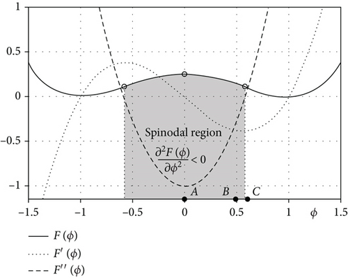
The results of equations (3) and (4), respectively, show that the conservation of total mass holds, and the total energy does not increase with respect to time. Figure 1 represents a double-well potential F(ϕ), its corresponding first and second derivatives. Here, the spinodal region is defined by the gray-colored region where the second derivative is negative, i.e., F^′′(ϕ) < 0. In this region, ϕ is unstable and then phase separation occurs. With these various applications of the CH equation, many researchers have proposed new efficient numerical methods [22–24]. Usually, in the stage of verifying the numerical method, the linear stability analysis is used. In [25], the linear stability was used for local equilibrium of Boltzmann equation. In [26], the stability analysis of the advective CH equation was employed to define the perturbation to investigate the instability of wave packets. In this paper, we shall present a clear standard for this test by defining linear and nonlinear regimes.

Details are in the caption following the image — **Figure 1**
Open in figure viewer PowerPoint

Schematic illustration of double-well potential F(ϕ), F^′(ϕ), and F^′′(ϕ).

The main purpose of this paper is to numerically investigate the dynamics of phase separation in binary mixtures with different average concentrations using the CH equation in the one-dimensional (1D) space. In addition, we propose criteria for linear regimes with small differences between numerical solutions and linear solutions.

This paper is organized as follows. The Fourier-spectral method is introduced in Section 2 for numerical solution. Section 3 provides numerical results and simulations with linear stability analysis. Conclusions are discussed in Section 4.

2. Numerical Solution

Now, we use the Fourier-spectral method [27] to find the numerical solution for the CH equation (1) in the 1D space Ω = (0, L),

(5)

Let h = L/N_x be the grid size in the x-axis directions, where N_x is positive even integer. At the edge points x_m = (m − 1)h where m = 1, 2, ⋯, N_x, we simply denote the numerical representation ϕ(x_m, t_n) into

. Here, t_n = nΔt and Δt is the temporal step size. Also, we set μ_p = 2πp/L for the Fourier-spectral method. Let us consider the discrete Fourier transform

and the inverse discrete Fourier transform

(6)

For simplicity of notation, we define f(ϕ) = F^′(ϕ) = ϕ³ − ϕ. By applying the linearly stabilized splitting scheme [28] into the CH equation (5), we obtain the following discrete CH equation:

(7)

Letting g(ϕ) = ϕ³ − 3ϕ, equation (7) comes into

(8)

Then, we can transform equation (8) into the discrete Fourier space as follows:

(9)

By rearranging the above one, we obtain

(10)

As a consequence, we can compute the updated numerical solution by applying the inverse discrete Fourier transform (6).

3. Numerical Experiments

In this section, we define growth rate of the CH equation and compare analytic growth rate with numerical growth rate. We also define an error between the analytic solution and the numerical solution. Through several numerical experiments about the growth rate and the error, we investigate the numerical behaviour at different spinodal points. Then, we propose linear and nonlinear regimes.

3.1. Analytic and Numerical Growth Rates

In this section, we shall find the analytic and numerical growth rates. We consider the following three different free energy functions [29], F₁, F₂, and F₃ at ϕ = ϕ_ave.

(11)

(12)

(13)

We linearize each of F′₁, F′₂, and F′₃ by applying the Taylor expansion for different free energy functions; then, we obtain the following linearized terms. The linearized functions are explained in detail in Appendix.

(14)

(15)

(16)

Therefore, for the free energy functions F₁, F₂, and F₃, the corresponding linear Cahn–Hilliard (LCH) equations are as follows:

(17)

(18)

(19)

To derive the ordinary differential equation for amplitude function α(t), we take ϕ(x, t) = ϕ_ave + α(t)cos(Kπx). For the positive even integer K, it can satisfy the periodic boundary condition. Substituting above ϕ(x, t) into LCH equations (17), (18), and (19), we have

(20)

(21)

(22)

Dividing cos(Kπx) on the both sides of equations (20), (21), and (22), we obtain

(23)

(24)

(25)

The analytic solutions of ordinary differential equations (23), (24), and (25) are as follows:

(26)

(27)

(28)

In this paper, we use F₁ unless the free energy function is mentioned; then, we write F₁ = F, λ₁ = λ. In the numerical approach, numerical growth rate is defined by

(29)

Here, ‖·‖_∞ denotes the maximum norm.

3.2. Convergence Test

In this section, we verify convergence of the numerical growth rate. For numerical test, we use ϕ(x, 0) = ϕ_ave + 0.001cos(10πx), ϕ_ave = 0, and ε = 0.02 in Ω = (0, 1).

Table 1 shows the numerical growth rate at time T = 0.004 for various Δt = T/N_t and h = 1/N_x. Here, the analytic growth rate is λ = 597.3241. In Table 1, we can see that the numerical growth rate converges to the analytic one as Δt and h decrease.

Table 1. Numerical growth rate for various Δt and h at T = 0.004 (λ = 597.3241).

N_t\N_x	2³	2⁴	2⁵	2⁶	2⁷
2¹¹	304.2649	594.2164	594.2139	594.2139	594.2139
2¹²	304.5360	595.7570	595.7545	595.7545	595.7545
2¹³	304.6718	596.5303	596.5278	596.5278	596.5278
2¹⁴	304.7397	596.9177	596.9152	596.9152	596.9152
2¹⁵	304.7737	597.1116	597.1091	597.1091	597.1091
2¹⁶	304.7907	597.2086	597.2061	597.2061	597.2061
2¹⁷	304.7992	597.2571	597.2546	597.2546	597.2546

3.3. Linear Stability Analysis

From now on, we implement the linear stability analysis with the constant solution ϕ = ϕ_ave. In the every numerical experiment, we use the constant to adjust the interfacial thickness. As long as do not more mentioned, the numerical parameters use such as N_x = 128, h = 1/N_x, Δt =2e-7, α(0) = 0.001, ε = ε₁₁, and T is total time. In addition, we use three different value ϕ_ave = 0, 0.4, and 0.6 which are in spinodal region and near critical points of free energy. Note that these values are indicated points A, B, and C in Figure 1. For a positive even integer K ≤ 16, the initial condition is selected as ϕ(x, 0) = ϕ_ave + 0.001cos(Kπx) in Ω = (0, 1). First, we investigate analytic and numerical growth rates for different mode numbers K.

Before the next tests, we define linear solution as follows:

(30)

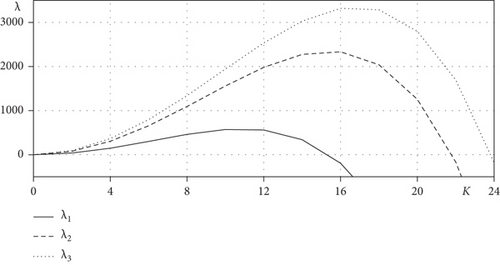
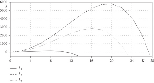
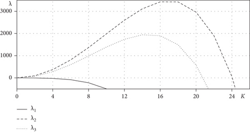
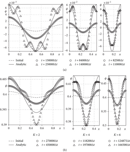
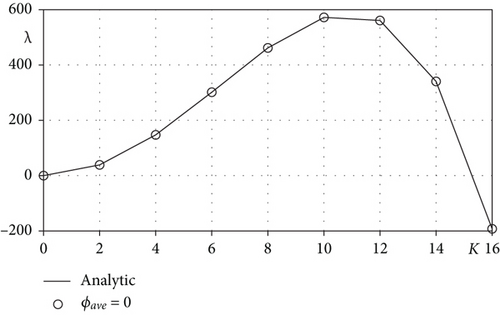
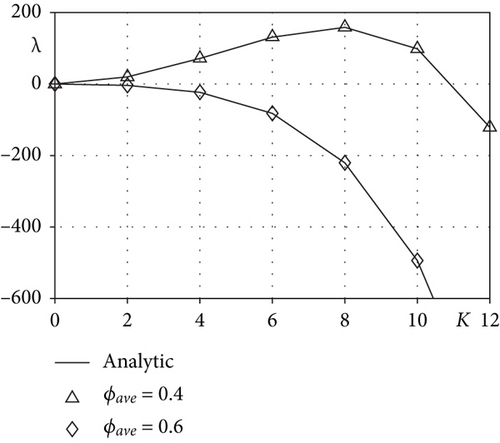
where α(t) = α(0)e^λt and λ is analytic growth rate, see equation (26). Figure 2 shows the change of the analytic and numerical growth rates with respect to each mode numbers K for ϕ_ave = 0, 0.4, and 0.6 in short-time evolution. As we can see, numerical growth rate

estimates analytic growth rate λ well in short time (T = 0.004). The growth rates in spinodal region (ϕ_ave = 0, ϕ_ave = 0.4) have positive values for some mode K. On the other hand (ϕ_ave = 0.6), the growth rates are always negative regardless of mode number K and also growth rates are monotonically decreased as mode number K increases. Figures 3(a)–3(c) show the analytic growth rates according to mode numbers K for ϕ_ave = 0, 0.4, and 0.6, respectively, where the analytic growth rates λ₁, λ₂, and λ₃ are (26), (27), and (28). However, in the long time evolution, it is difficult to expect the numerical growth rate that fits well with the analytic one. In order to find this reason, we first observe dynamics of the numerical solution ϕ(x, t) and linear solution u(x, t). In Figure 4, we can check the behaviour of the numerical and linear solution in short and long time evolution for K = 2, 4, and 6, when ϕ_ave = 0 and ϕ_ave = 0.4. Unlike the short-time cases, the long-time numerical solutions in all cases show a lot of difference from the linear solutions. This result means that over time, the CH solution has nonlinearity.

Let us consider Ginzburg–Landau free energy (2) by decomposing it as

(31)

where

(32)

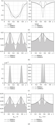
We compare short- and long-time numerical solution ϕ(x, t) when ϕ_ave = 0 and ϕ_ave = 0.4. In this test, we use mode K = 2 and α(0) = 0.1. As shown in Figure 5(a), we can see the nonlinearity in the long-time solution after a certain period of time, regardless of ϕ_ave. Figures 5(b)–5(d) show results of double well potential F(ϕ), ε/2|∇ϕ|², and F(ϕ) + ε/2|∇ϕ|², respectively. Here, the solid and dashed lines mean the short- and long-time results of each function, respectively. Also, the area of the gray-colored region in Figures 5(b)–5(d) represent the energy , , and the Ginzburg–Landau free energy , respectively.

As shown in Figure 1, as ϕ moves away from ϕ = 0, F(ϕ) becomes smaller than F(0) when −1 ≤ ϕ ≤ 1. For this result, in Figure 5(b), dashed line is located below solid line overall of x. It means that F(ϕ) becomes smaller over time in the spinodal region. Also, according to fluctuation of ϕ, we can see the property of ε²/2|∇ϕ|² in Figure 5(c). However, it can also be confirmed that the value has a slight effect on F(ϕ) + ε/2|∇ϕ|² as shown in Figure 5(d). In conclusion, we know that the CH solution grows with time in the spinodal region, and it has nonlinearity in the existing solution in order to reduce the total free energy.

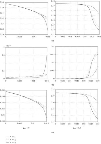
Figures 6(a)–6(c) show temporal evolution of , , and with different ε. All results of and decrease with respect to time t. However, it can be seen that the larger the epsilon, that is, the thicker the interface of numerical solution, the slower the result is expressed.

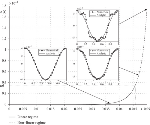
From now on, we verify that the CH solution has nonlinearity over time. Therefore, when performing a linear stability test, it is accurate to examine short time evolution. Also, based on this fact, we propose the criteria for defining the following linear and nonlinear regimes. To find linear regime where numerical solution estimates linear solution well, we define error e(nΔt) between numerical and linear solution as follows:

(33)

We can distinguish linear regime and nonlinear regime based on the user-criteria tol as follows: if e(nΔt) < tol; then, linear regime; otherwise, non-linear regime. We propose a criterion tol using the initial condition u(x, 0) as follows:

(34)

Figure 7 shows proposed criterion and temporal evolution of error e(t = nΔt) for the time t with dynamic of linear and numerical solutions.

4. Conclusions

We studied a linear stability analysis for the CH equation in spinodal region as different average levels. To solve the CH equation, we used linearly stabilized splitting scheme and Fourier-spectral method. Through the numerical simulations, we observed various dynamics of the CH equation and confirmed the numerical solution compared linear solution over time. We defined growth rate and also compared numerical growth rate and analytic growth rate. Using difference between numerical and linear solution, we defined error. By means of defined error, we distinguish linear regime where numerical solution and linear solution match because of the small error and nonlinear regime where do not.

Conflicts of Interest

The authors declare that they have no conflicts of interest.

Acknowledgments

The first author (S. Ham) was supported by the Brain Korea 21 FOUR through the National Research Foundation of Korea funded by the Ministry of Education of Korea. This study was supported by 2020 Research Grant from Kangwon National University. The author (D. Jeong) was supported by the National Research Foundation of Korea (NRF) grant funded by the Korea government (MSIP) (NRF-2020R1F1A1A01075937). The corresponding author (J.S. Kim) was supported by Basic Science Research Program through the National Research Foundation of Korea (NRF).

Appendix

A. Appendix: Linearlization

By the Taylor theorem, for real valued-function f(x), if f(x) has derivatives of all orders at a, then for each positive integer n,

(A.1)

where

Now, we approximate the linearized functions of various free energies at ϕ_ave.

(A.2)

(A.3)

(A.4)

Open Research

Data Availability

No data were used to support this study.

References

1 Cahn J. W., Über die umsetzung an der spinodalen, Acta Metallurgica. (1961) 9, no. 9, 795–801, https://doi.org/10.1016/0001-6160(61)90182-1, 2-s2.0-43449102981.
10.1016/0001-6160(61)90182-1
CAS Web of Science® Google Scholar
2 Cahn J. W. and Hilliard J. E., Spinodale entmischung: Eine reprise, Acta Metallurgica. (1971) 19, no. 2, 151–161, https://doi.org/10.1016/0001-6160(71)90127-1, 2-s2.0-0015018902.
10.1016/0001-6160(71)90127-1
CAS Web of Science® Google Scholar
3 Erlebacher J., Aziz M. J., Karma A., Dimitrov N., and Sieradzki K., Evolution of nanoporosity in dealloying, Nature. (2001) 410, no. 6827, 450–453, https://doi.org/10.1038/35068529, 2-s2.0-0035932448, 11260708.
10.1038/35068529
CAS PubMed Web of Science® Google Scholar
4 Khenner M. and Henner V., Modeling evolution of composition patterns in a binary surface alloy, Modelling and Simulation in Materials Science and Engineering. (2021) 29, no. 1, https://doi.org/10.1088/1361-651X/abc301.
10.1088/1361-651X/abc301
Web of Science® Google Scholar
5 Menshov I. S. and Zhang C., Interface capturing method based on the Cahn–Hilliard equation for two-phase flows, Computational Mathematics and Mathematical Physics. (2020) 60, no. 3, 472–483, https://doi.org/10.1134/S0965542520030124.
10.1134/S0965542520030124
Web of Science® Google Scholar
6 Yang J. and Kim J., A novel Cahn-Hilliard-Navier-Stokes model with a nonstandard variable mobility for two-phase incompressible fluid flow, Computers and Fluids. (2020) 213, https://doi.org/10.1016/j.compfluid.2020.104755.
10.1016/j.compfluid.2020.104755
Web of Science® Google Scholar
7 Yang J. and Kim J., An efficient stabilized multiple auxiliary variables method for the Cahn- Hilliard-Darcy two-phase flow system, Computers and Fluids. (2021) 223, https://doi.org/10.1016/j.compfluid.2021.104948.
10.1016/j.compfluid.2021.104948
Web of Science® Google Scholar
8 Zhou S. and Wang M. Y., Multimaterial structural topology optimization with a generalized Cahn-Hilliard model of multiphase transition, Structural and Multidisciplinary Optimization. (2006) 33, no. 2, 89–111, https://doi.org/10.1007/s00158-006-0035-9, 2-s2.0-33845955558.
10.1007/s00158-006-0035-9
Web of Science® Google Scholar
9 Zhang X., Takezawa A., and Kang Z., A phase-field based robust topology optimization method for phononic crystals design considering uncertain diffuse regions, Computational Materials Science. (2019) 160, 159–172, https://doi.org/10.1016/j.commatsci.2018.12.057, 2-s2.0-85059680981.
10.1016/j.commatsci.2018.12.057
CAS Web of Science® Google Scholar
10 Bartels A., Kurzeja P., and Mosler J., Cahn-Hilliard phase field theory coupled to mechanics: fundamentals, numerical implementation and application to topology optimization, Computer Methods in Applied Mechanics and Engineering. (2021) 383, https://doi.org/10.1016/j.cma.2021.113918.
10.1016/j.cma.2021.113918
Web of Science® Google Scholar
11 Cohen D. and Murray J. M., A generalized diffusion model for growth and dispersal in a population, Journal of Mathematical Biology. (1981) 12, no. 2, 237–249, https://doi.org/10.1007/BF00276132, 2-s2.0-0019870511.
10.1007/BF00276132
Web of Science® Google Scholar
12 Aristotelous A. C., Karakashian O. A., and Wise S. M., Adaptive, second-order in time, primitive-variable discontinuous Galerkin schemes for a Cahn-Hilliard equation with a mass source, IMA Journal of Numerical Analysis. (2015) 35, no. 3, 1167–1198, https://doi.org/10.1093/imanum/dru035, 2-s2.0-84939519549.
10.1093/imanum/dru035
Web of Science® Google Scholar
13 Feng W., Guo Z., Lowengrub J. S., and Wise S. M., A mass-conservative adaptive FAS multigrid solver for cell-centered finite difference methods on block-structured, locally-cartesian grids, Journal of Computational Physics. (2018) 352, 463–497, https://doi.org/10.1016/j.jcp.2017.09.065, 2-s2.0-85031490811.
10.1016/j.jcp.2017.09.065
Web of Science® Google Scholar
14 Agosti A., Antonietti P. F., Ciarletta P., Grasselli M., and Verani M., A Cahn–Hilliardtype equation with application to tumor growth dynamics, Mathematical Methods in the Applied Sciences. (2017) 40, no. 18, 7598–7626, https://doi.org/10.1002/mma.4548, 2-s2.0-85058456210.
10.1002/mma.4548
Web of Science® Google Scholar
15 Oron A., Davis S. H., and Bankoff S. G., Long-scale evolution of thin liquid films, Reviews of Modern Physics. (1997) 69, no. 3, 931–980, https://doi.org/10.1103/RevModPhys.69.931.
10.1103/RevModPhys.69.931
CAS Web of Science® Google Scholar
16 Thiele U. and Knobloch E., Thin liquid films on a slightly inclined heated plate, Physica D. (2004) 190, no. 3-4, 213–248, https://doi.org/10.1016/j.physd.2003.09.048, 2-s2.0-1142303895.
10.1016/j.physd.2003.09.048
Web of Science® Google Scholar
17 Torabi S. and Lowengrub J., Simulating interfacial anisotropy in thin-film growth using an extended Cahn–Hilliard model, Physical Review E. (2012) 85, no. 4, https://doi.org/10.1103/PhysRevE.85.041603, 2-s2.0-84860535057, 22680484.
10.1103/PhysRevE.85.041603
PubMed Web of Science® Google Scholar
18 Choksi R., Peletier M. A., and Williams J. F., On the phase diagram for microphase separation of diblock copolymers: an approach via a nonlocal Cahn-Hilliard functional, SIAM Journal on Applied Mathematics. (2009) 69, no. 6, 1712–1738, https://doi.org/10.1137/080728809, 2-s2.0-66049155985.
10.1137/080728809
CAS Web of Science® Google Scholar
19 Jeong D. and Kim J., Microphase separation patterns in diblock copolymers on curved surfaces using a nonlocal Cahn–Hilliard equation, The European Physical Journal E. (2015) 38, no. 11, 1–7, https://doi.org/10.1140/epje/i2015-15117-1, 2-s2.0-84947437391.
10.1140/epje/i2015-15117-1
CAS PubMed Web of Science® Google Scholar
20 Bertozzi A., Esedoglu S., and Gillette A., Inpainting of binary images using the Cahn-Hilliard equation, IEEE Transactions on Image Processing. (2007) 16, no. 1, 285–291, https://doi.org/10.1109/TIP.2006.887728, 2-s2.0-33847721052, 17283787.
10.1109/TIP.2006.887728
PubMed Web of Science® Google Scholar
21 Bertozzi A., Esedoglu S., and Gillette A., Analysis of a two-scale Cahn-Hilliard model for binary image inpainting, Multiscale Modeling and Simulation. (2007) 6, no. 3, 913–936, https://doi.org/10.1137/060660631, 2-s2.0-50949104589.
10.1137/060660631
Web of Science® Google Scholar
22 Li Y., Jeong D., Shin J., and Kim J., A conservative numerical method for the Cahn-Hilliard equation with Dirichlet boundary conditions in complex domains, Computers & Mathematcs with Applications. (2013) 65, no. 1, 102–115, https://doi.org/10.1016/j.camwa.2012.08.018, 2-s2.0-84871389895.
10.1016/j.camwa.2012.08.018
Web of Science® Google Scholar
23 Li Y., Lee H. G., Xia B., and Kim J., A compact fourth-order finite difference scheme for the three-dimensional Cahn-Hilliard equation, Computer Physics Communications. (2016) 200, 108–116, https://doi.org/10.1016/j.cpc.2015.11.006, 2-s2.0-84957428815.
10.1016/j.cpc.2015.11.006
CAS Web of Science® Google Scholar
24 Li Y., Choi Y., and Kim J., Computationally efficient adaptive time step method for the Cahn-Hilliard equation, Computers & Mathematcs with Applications. (2017) 73, no. 8, 1855–1864, https://doi.org/10.1016/j.camwa.2017.02.021, 2-s2.0-85015660095.
10.1016/j.camwa.2017.02.021
Web of Science® Google Scholar
25 Di Y., Fan Y., Li R., and Zheng L., Linear stability of hyperbolic moment models for Boltzmann equation, Numerical Mathematics: Theory, Methods and Applications. (2017) 10, no. 2, 255–277, https://doi.org/10.4208/nmtma.2017.s04, 2-s2.0-85019103530.
10.4208/nmtma.2017.s04
Web of Science® Google Scholar
26 Barletta A. and Celli M., Unstable wave-packet perturbations in an advective Cahn–Hilliard process, Physical Review E. (2019) 99, no. 5, https://doi.org/10.1103/PhysRevE.99.052219, 2-s2.0-85066424843.
10.1103/PhysRevE.99.052219
PubMed Web of Science® Google Scholar
27 Shen J., Tang T., and Wang L. L., Spectral methods: algorithms analysis and applications, Springer Science & Business Media. (2011) 41, 23–46.
Google Scholar
28 Lee S., Lee C., Lee H. G., and Kim J., Comparison of different numerical schemes for the Cahn–Hilliard equation, Journal of the Korean Society for Industrial and Applied Mathematics. (2013) 17, no. 3, 197–207, https://doi.org/10.12941/jksiam.2013.17.197.
10.12941/jksiam.2013.17.197
Google Scholar
29 Shah A., Sabir M., and Ayub S., An adaptive time-stepping scheme for the numerical simulation of Cahn-Hilliard equation with variable mobility, Journal of applied mathematics and mechanics. (2019) 99, no. 7, https://doi.org/10.1002/zamm.201800246, 2-s2.0-85065061832.
10.1002/zamm.201800246
Google Scholar

All articles

Linear Stability Analysis of the Cahn–Hilliard Equation in Spinodal Region

Abstract

1. Introduction

2. Numerical Solution